Vortex-Line Phase Diagram for Anisotropic Superconductors

Abstract

The zero temperature vortex phase diagram for uniaxial anisotropic superconductors placed in an external magnetic field tilted with respect to the axis of anisotropy is studied for parameters typical of BSCCO and YBCO. The exact Gibbs free energy in the London approximation, using a self-energy expression with an anisotropic core cutoff, is minimized numerically, assuming only that the equilibrium vortex state is a vortex-line-lattice with a single vortex line per primitive unit cell. The numerical method is based on simulated annealing and uses a fast convergent series to calculate the energy of interaction between vortex lines. A phase diagram with three distinct phases is reported and the phases are characterized in detail. New results for values of the applied field close to the lower critical field are reported.

I Introduction

One important theoretical problem in the study of type-II superconductors is the zero temperature equilibrium vortex phase diagram for clean, uniaxially anisotropic, bulk materials subjected to an external magnetic field, ${\bf H}$ tilted with respect to the axis of anisotropy ($c$-axis). In the case of isotropic materials the vortex phase is the well known triangular vortex-line lattice with the vortex lines oriented parallel to ${\bf H}$. In anisotropic materials the vortex phase is still a vortex-line lattice but, in general, the lattice is not triangular nor are the vortex lines oriented along ${\bf H}$ [1, 2].

Previous work find that the vortex phases for the anisotropic superconductor are related to those for the isotropic one when ${\bf H}$ is oriented along the c-axis, in which case they are identical, when ${\bf H}$ is along the a-b plane or for $H$ large compared with the lower critical field [3]. In the latter two cases, the vortex-line-lattices are related to the triangular lattice by scaling and the vortex lines are essentially parallel to ${\bf H}$. For general orientations of ${\bf H}$ this is not the case. The vortex phases were first obtained by Buzdin and Simonov [4] by numerically minimizing the Gibbs free-energy in the London limit with material parameters appropriate for YBCO. Our calculation, like their’s, minimizes the London Gibbs free-energy numerically. However, we go beyond the work of these authors by incorporating into our calculations recent results for the vortex state at the lower critical field, not taken into account by them [5, 6]. We show that this leads to new vortex phases close to the lower critical field.

It was found first by Grishin, Martynovich and Yampol’skii [7] and later by others [8, 9, 10], that a pair of straight vortex lines parallel to each other and coplanar with respect to the c-axis attract at large distances. A consequence of this is that a chain of such lines has lower energy than the same vortex lines placed far apart. On the basis of this result Buzdin and co-workers [8, 10] suggested that at the lower critical field the mixed state consists of a vanishing small density of vortex line chains instead of vortex lines. However this argument does not apply in general. As pointed out in Ref.[6], in order to determine whether vortex lines or vortex-line chains constitute the vortex phase at the lower critical field it is necessary to minimize the Gibbs free-energy for each one of them and obtain their respective lower critical fields. The one with the lower critical field is the true equilibrium phase. One important aspect of the calculation of Ref.[6] is the use of an expression for the tilted vortex-line self energy with an appropriate anisotropic core cutoff function. This expression was derived by Subdo and Brandt [11] and later used in Ref.[5] to show, by minimizing the London Gibbs free-energy for a vanishing small density of vortex lines, that for anisotropy parameters typical of BSCCO there is coexistence two such states, with different vortex lines tilt angles, for one particular orientation of ${\bf H}$. These authors also showed that if a self-energy expression based on an isotropic core cutoff, such as the one adopted by Buzdin and Simonov [8], is used instead, the coexistence disappears. It is found in Ref.[6] that at the lower critical field and for anisotropy parameters typical of BSCCO the equilibrium vortex state for ${\bf H}$ tilted by $\alpha<\alpha_{c}=7.9^{o}$ with respect to the c-axis is a dilute vortex-line chain state whereas for $\alpha>\alpha_{c}=7.9^{o}$ it is a dilute vortex-line one. For anisotropy parameters typical of YBCO Ref.[6] finds that the lower critical fields for vortex lines and vortex-line chains differ so little from each other that it is not possible do decide which one corresponds to true equilibrium.

In this paper, we minimize the exact Gibbs free-energy in the London limit using Sudbo and Brandt [11] expression the vortex line self energy. We assume that the equilibrium state the vortex lines are straight and parallel to each other and the VLL has only one vortex line per unit cell, and obtain the vortex lines orientation and VLL shape as functions of ${\bf H}$, by minimizing the Gibbs free-energy in the London limit.

The free parameters in our calculation for given ${\bf H}$, specified here by its magnitude, $H$, and its tilt angle with respect to the c-axis, $\alpha$, are the vortex lines tilt angle, $\theta$, and the VLL primitive unit cell vectors ${\bf L_{1}}$ and ${\bf L_{2}}$, defined in the plane perpendicular to the vortex lines. Since the vortex lines are straight and parallel to each other, the magnetic induction ${\bf B}$ is also tilted by $\theta$ with respect to the c-axis and, as explained in detail in Sec. II A, it is coplanar with ${\bf H}$ and the c-axis. The orientations of ${\bf H}$, ${\bf B}$, and the c-axis, and the VLL primitive unit cell are shown in Fig. 1. Hereafter we specify the VLL unit cell by the magnitudes of ${\bf L_{1}}$ and ${\bf L_{2}}$, denoted by $L_{1}$ and $L_{2}$, by the angle between ${\bf L_{1}}$ and ${\bf L_{2}}$, $\varphi$, and by and the angle of rotation of the VLL unit cell with respect to ${\bf B}$, $\psi$, as shown in Fig. 1.

As discussed in Sec. II A, a minimum of the Gibbs free-energy occurs for $\psi=0$, where $\psi$ is defined in Fig. 1. We assume that this is the absolute minimum and carry out the calculations with $\psi=0$. This means that ${\bf L_{1}}$ is also coplanar with ${\bf H}$ and the c-axis,oriented along the x-direction defined in Fig. 1. To simplify the calculations we set $\varphi=90^{o}$. This means that the VLL unit cell is a rectangle, with ${\bf L_{2}}$ perpendicular to the plane defined by ${\bf H}$, ${\bf B}$ and the c-axis (Fig. 1). We find that this simplifications does not change our main results. Under these conditions we have only three free parameters, to be determined by minimizing the Gibbs free-energy: $\theta$, $L_{1}$ and $L_{2}$. This minimization is carried out numerically, using a fast convergent series to calculate lattice sums entering the expression for the VLL interaction energy [13]. This series, together with the small number of free parameters, allow us to create an efficient and accurate numerical algorithm.

We study in detail the phase diagram for anisotropy parameters typical of YBCO and BSCCO. For YBCCO our results are essentially the same as those obtained by Buzdin and Simonov, except very close to the lower critical field. For BSCCO our results are new.

The main results of this paper are summarized in the generic phase diagram show in Fig. 2. We find three distinct phases, hereafter called phase-I, phase-II, and phase-III. We find that phase-I is new and closely related to the vortex-line equilibrium state at the lower critical field. We also find that phase- II is essentially identical to that found by Buzdin and Simonov and that phase-III is that expected for fields much larger than the lower critical field. In this limit the VLL unit cell is related to that appropriate for the isotropic superconductor by scaling, and ${\bf B}\simeq{\bf H}$ ($\theta\simeq\alpha$) [3].

The lower critical field in isotropic superconductors is independent of the orientation $(\alpha)$, and has magnitude $H_{c1}$. For $H$ just above $H_{c1}$, the vortex state corresponds to vortex lines parallel to ${\bf H}$ very far apart. In our notation this state is described by $\theta=\alpha$ and $L_{1}$, $L_{2}=\infty$. In a superconductor with uniaxial anisotropy, the magnitude of the lower critical field depends on $\alpha$, hereafter denoted by $H_{c1}(\alpha)$ [5]. The vortex state for $H$ just above $H_{c1}(\alpha)$ consists of vortex lines not parallel to ${\bf H}$ ($\theta\neq\alpha$) in one of two possible configurations, named dilute vortex line state (DVL) and dilute vortex-line chain state (DVLC) [6]. The DVL is similar to the traditional vortex state for the isotropic superconductor, in the sense that $L_{1}$, $L_{2}=\infty$, whereas the DVLC corresponds to vortex-line chains along the x-direction with period $L_{1}$, very far apart, that is $L_{1}$ finite and $L_{2}=\infty$. The latter possibility results from attractive interactions between vortex lines that only exist in anisotropic superconductors [7, 8, 9, 10]. To decide if the DVL or the DVLC is the equilibrium vortex state it is necessary to calculate $H_{c1}(\alpha)$ for each one. The equilibrium configuration is that with the smallest $H_{c1}(\alpha)$. This calculation is reported in Ref.[6]. The results for anisotropy parameters typical of BSCCO and YBCO, referred to as strong an moderate anisotropies, respectively, are shown in Fig. 3. It is found that for both anisotropies there is a value of the external field tilt angle, $\alpha_{c}$, around which the equilibrium vortex states undergoes a significant change. For $\alpha>\alpha_{c}$ and both for strong and moderate anisotropies the equilibrium state is a DVL with vortex lines tilted at $\theta\simeq 90^{o}$, that is parallel to the ab-plane. For strong anisotropy the vortex state for $\alpha<\alpha_{c}=7.9^{o}$ is a DVLC with vortex lines tilted at $\theta<60^{o}$. At $\alpha=\alpha_{c}$, there is coexistence of a DVL and DVLC. A discontinuous change in $\theta$ takes place at $\alpha=\alpha_{c}$. For a moderate anisotropy, $\theta$ is found to change smoothly with $\alpha$ and $\alpha_{c}\sim 20^{o}$. The calculation on Ref.[6] finds that for moderate anisotropy the DVL and DVLC values of $H_{c1}(\alpha)$ are so close that their difference is within the numerical errors of the calculation.

We find that phases I and II evolve, respectively, from the $\alpha<\alpha_{c}$ and $\alpha>\alpha_{c}$ vortex states at $H=H_{c1}(\alpha)$, represented by the horizontal line in Fig. 2.

Phase-II is essentially an extension into the $H>H_{c1}(\alpha)$ region of the phase diagram of the vortex state found for $\alpha>\alpha_{c}$ at $H=H_{c1}(\alpha)$. Its predominant characteristic is that $\theta\sim 90^{o}$ and, consequently, the VLL within phase-II is essentially identical to that for vortex lines parallel to the ab-plane. In this case the unit cell is, approximately, related to that for the isotropic superconductor by scaling relations that depend only on the anisotropy. For strong and moderate anisotropies the unit cell is a rectangle elongated in the y-direction, that is $L_{1}\gg L_{2}$. Phase-II is limited from above by the line $H=H^{*}(\alpha)$, which gives the field value around which $\theta$ changes from $90^{o}$ to a lower value, accompanied by significant changes in the VLL unit cell. At $\alpha=\alpha_{c}$, $H^{*}(\alpha)=H_{c1}(\alpha)$.

Phase-I is the region of the phase diagram where the VLL properties are strongly influenced by the attractive interactions between pairs of vortex lines aligned along the x-directions. For both strong and moderate anisotropies we find that phase-I is not limited to $\alpha<\alpha_{c}$, but it also exists in a small part of the region $\alpha>\alpha_{c}$ and $H>H^{*}(\alpha)$. For strong anisotropy we find that phase-I consists of vortex-line chains along the x-direction, with a period $L_{1}$ that is nearly identical to that of an isolated chain with the same tilt angle (which differs from that of an isolated vortex), separated from each other by $L_{2}\gg L_{1}$. This means that the attractive interactions between vortex lines prevail in determining the VLL periodicity along the x-direction. We also find that as $H\rightarrow H_{c1}(\alpha)$ from above, the equilibrium VLL approaches the same DVLC found in Ref.[6] for $H=H_{c1}(\alpha)$. For moderate anisotropy we obtain a new result for the vortex state at $H=H_{c1}(\alpha)$. By extrapolating our data as $H\rightarrow H^{*}(\alpha)$ from above, we conclude that the vortex state at $H=H_{c1}(\alpha)$ is a DVLC. However, within phase-I for moderate anisotropy, the attractive interactions between vortex lines are so weak that vortex-line chains along the x-direction with periods close to those of isolated chains only exist within phase-I near $H=H_{c1}(\alpha)$. However, distinctive behavior, due to attractive vortex-line interactions, can still be identified within phase-I.

This paper is organized as follows. In Sec. II A we review London theory for the energy of the vortex-line system under consideration and the known results for the phase diagram at $H=H_{c1}(\alpha)$ and for particular cases at $H>H_{c1}(\alpha)$. In Sec. II B we discuss the numerical method used to minimize the Gibbs free energy. In Sec. III we report the results of this minimization, the detailed properties of each phase, and discuss how the phases are identified. Our conclusions are stated in Sec. IV. In the Appendix the relevant formulas for the fast convergent series used in our in our calculation are summarized.

II Method of Calculation

Here, we review London theory for this problem, its known results for the phase diagram, and describe some details of our numerical method.

A London Theory

To obtain the zero-temperature phase diagram for a superconductor in an applied field it is necessary to determine the vortex arrangement that minimizes the Gibbs free-energy density

$$G=F-\frac{{\bf H}\cdot{\bf B}}{4\pi}\;$$ (1)

with ${\bf H}$ and the volume kept constant. In Eq. (1) $F$ is the vortex energy density and ${\bf B}$ is the magnetic induction. We assume that the zero-temperature equilibrium vortex configuration consist of straight vortex lines, parallel to each other, arranged on a periodic VLL, with a single vortex line per primitive unit cell. In this case ${\bf B}$ is parallel to the vortex lines direction and has magnitude $B=\Phi_{0}/A_{c}$, where $A_{c}$ is the VLL primitive unit cell area. Minimization of $G$ gives then the vortex lines orientation and unit cell shape that corresponds to equilibrium. Because $F$ is unchanged, if the vortex lines are rotated around the $c$-axis, the equilibrium ${\bf B}$ lies in the same plane as ${\bf H}$ and the $c$-axis. Thus, for ${\bf H}$ with magnitude $H$ and tilted with respect to the $c$-axis by an angle $\alpha$, $G$ depends on the vortex lines tilt angle with respect to the $c$-axis, $\theta$, and on the parameters defining the VLL primitive unit cell. In the system of axis defined in Fig. 1.a, the generic VLL primitive unit cell lies in the $x-y$ plane, and is defined by the primitive unit vectors ${\bf L_{1}}$ and ${\bf L_{2}}$, as shown in Fig. 1.b. In this case $A_{c}=L_{1}L_{2}\sin{\varphi}$.

In the London limit the superconductor is characterized by the penetration depths $\lambda_{ab}$ and $\lambda_{c}$, for currents parallel to the $ab$-plane and to the $c$-direction, respectively. The free energy density of a generic arrangement of these vortex lines can be written as the sum of pairwise interactions [2]

$$F=\frac{\Phi^{2}_{0}}{8\pi A}\sum_{i,j}f({\bf r}_{i}-{\bf r}_{j})\;,$$ (2)

where ${\bf r}_{i}$ is the i-th vortex-line position vector in $x-y$ plane, $A$ is the sample area in this plane, and $f({\bf r})$ is the Fourier transform of

$$f({\bf k})=e^{-2g(\bf k)}\;\frac{1+\lambda^{2}_{\theta}k^{2}}{(1+\lambda^{2}_{ab}k^{2})(1+\lambda^{2}_{\theta}k^{2}_{x}+\lambda^{2}_{c}k^{2}_{y})}\;,$$ (3)

where

$$\lambda^{2}_{\theta}=\lambda^{2}_{ab}\sin^{2}{\theta}+\lambda^{2}_{c}\cos^{2}{\theta}\;,$$ (4)

and $g(\bf k)$ is the vortex core cutoff function [2, 3]. It is costumery to write $G$ as

$$G(\theta,{\bf L_{1}},{\bf L_{2}};{\bf H})=\frac{B}{\Phi_{0}}[\varepsilon_{\rm sf}(\theta)+\varepsilon_{\rm in}(\theta,{\bf L_{1}},{\bf L_{2}})-\frac{\Phi_{0}}{4\pi}H\cos{(\theta-\alpha)}]\;,$$ (5)

where $\varepsilon_{\rm sf}(\theta)$ is the vortex line self-energy and $\varepsilon_{\rm in}(\theta,{\bf L_{1}},{\bf L_{2}})$ is the interaction energy per vortex line. In terms of $f({\bf r})$, defined in Eq. (2), these quantities are given by

$$\varepsilon_{sf}(\theta)=\frac{\Phi_{0}}{8\pi}f({\bf r}=0)\;,$$ (6)

and

$$\varepsilon_{in}=\frac{\Phi_{0}}{8\pi}\sum_{i\neq j}f({\bf R}_{i}-{\bf R}_{j})\;,$$ (7)

where ${\bf R}_{i}$ denotes the VLL positions (${\bf R}_{i}=n_{1}{\bf L}_{1}+n_{2}{\bf L}_{2}$, $n_{1}$, $n_{2}=$ integer).

The minima of $G$, Eq. (5), are known in the following cases.

i) Lower critical field: $H=H_{c1}(\alpha)$. The equilibrium vortex phase at the lower critical field is studied by Sudbø, Brandt and Huse [5], assuming that it consists of a dilute arrangement of straight vortex lines (DVL). Accordingly, these authors minimize $G$, Eq. (5), neglecting $\varepsilon_{\rm in}$, and using for $\varepsilon_{\rm sf}$ the expression derived by Sudbø, and Brandt [11], based on an elliptic core cutoff function,

$$\varepsilon_{\rm sf}(\theta)=\varepsilon_{0}\frac{\lambda_{\theta}}{\lambda_{c}}[\ln({\kappa}/{\gamma})+\frac{\lambda^{2}_{c}\cos^{2}{\theta}}{\lambda^{2}_{c}\cos^{2}{\theta}+\lambda^{2}_{\theta}}\ln{\frac{\gamma^{2}(\lambda^{2}_{c}+\lambda^{2}_{\theta})}{2\lambda^{2}_{\theta}}}]\;,$$ (8)

where $\varepsilon_{0}=(\Phi_{0}/4\pi\lambda_{ab})^{2}$, $\gamma=\lambda_{ab}/\lambda_{c}=\xi_{c}/\xi_{ab}$, $\kappa=\lambda_{ab}/\xi_{ab}$, $\xi_{ab}$ being the $ab$-plane coherence length. This line energy is obtained from the anisotropic Ginzburg-Landau theory using the Klemm-Clem transformation [11, 12]. The elliptical core cutoff has semi major axis $\xi^{-1}_{ab}$ and semi minor axis $\xi^{-1}_{\theta}$ with $\xi^{2}_{\theta}=\xi^{2}_{ab}\cos^{2}{\theta}+\xi^{2}_{c}\sin^{2}{\theta}$. Sudbø, Brandt and Huse [5] obtain $H_{c1}(\alpha)$ for several values of the anisotropy parameter $\gamma$ and of $\kappa$, and find that for certain ranges of $\gamma$ and $\kappa$, there is a value of $\alpha$, $\alpha=\alpha_{c}$, for which coexistence of two DVL differing from each other by the equilibrium $\theta$ takes place.

In a recent publication by some of us [6], the Sudbø, Brandt and Huse [5] calculation was generalized to account for two possible vortex phases at the lower critical field: a dilute vortex-line state (DVL) considered by them and a dilute vortex-line chains arrangement (DVLC). The DVLC consists of vortex lines tilted with respect to the $c$-axis, parallel to one another, and aligned along the x-direction, forming a periodic chain. This is possible because the interaction between a pair of such vortices is attractive at large distances [7, 8, 9, 10]. In Ref:[6], $G$, Eq. (5), is minimized in the limit of vanishing vortex density, for each one of these possibilities. For the DVL, $\varepsilon_{\rm int}$ is neglected in Eq. (5), whereas for the DVLC $\varepsilon_{\rm int}$ in Eq. (5) is identified with the interaction energy per vortex line of an isolated chain. The lower critical field as a function of the tilt angle $\alpha$, $H_{c1}(\alpha)$ is then obtained for each possibility, and the equilibrium vortex phase at $H=H_{c1}(\alpha)$ is identified as that with the smallest $H_{c1}(\alpha)$.

In Ref:[6], two sets of anisotropy parameters are considered:

Strong anisotropy: $\kappa=10$, $\gamma=1/\surd{200}$

Moderate anisotropy: $\kappa=50$, $\gamma=1/5$

These values for $\gamma$ are typical of YBCO (moderate anisotropy) and BSCCO (strong anisotropy). The parameter $\kappa$ for moderate anisotropy is typical of YBCO but for strong anisotropy is about five times smaller than those typical of BSCCO [1]. However, this difference does not alter significantly the phase diagram because only the self-energy depends on $\kappa$.

The main results of Ref.[6], summarized in Fig. 3 are as follows. For both moderate and strong anisotropy and for $\alpha>\alpha_{c}$ the vortex lines are nearly parallel to the a-b plane ($\theta\sim 90^{o}$). For strong anisotropy $\alpha_{c}=7.9^{o}$ and for moderate anisotropy $\alpha\sim 20^{o}$. For strong anisotropy and $\alpha<\alpha_{c}$ the vortex phase at $H=H_{c1}(\alpha)$ is a DVLC. For $\alpha>\alpha_{c}$, on the other hand, no significant difference is found between the DVLC and DVL phases, because the vortex lines are tilted at $\theta\sim 90^{o}$, and at such tilt angles the equilibrium chain period is very large. Phase coexistence is also found for strong anisotropy at $\alpha=\alpha_{c}=7.9^{o}$, but the coexisting phases are a DVLC and DVL, instead of the two DVL found in Ref.[5]. A discontinuous jump in $\theta$ takes place as $\alpha$ crosses $\alpha_{c}=7.9^{o}$. For moderate anisotropy the DVL and DVLC phases give nearly identical values for $H_{c1}(\alpha)$, so that no conclusion on which is the equilibrium state is reached.

ii) $\alpha=0^{o}$ $and$ $\alpha=90^{o}$. In both cases $\theta=\alpha$ and the lower critical field is related to the self energy by the usual formula $H_{c1}(\alpha=0^{o},90^{o})=4\pi\varepsilon_{\rm sf}(\theta=0^{o},90^{o})/\Phi_{0}$. For $\alpha=\theta=0^{o}$ the equilibrium VLL is the familiar isotropic superconductor triangular lattice, with $L_{1}=L_{2}=L_{\Delta}\equiv(\Phi_{0}/B\sin{60^{o}})^{1/2}$, $\varphi=60^{o}$ and $\psi$ undetermined. For $\alpha=\theta=90^{o}$ the x-direction coincides with the negative $c$-axis. The equilibrium VLL is related to that for $\alpha=\theta=0^{o}$ (assuming ${\bf L}_{1}$ along the x-direction or $\psi=0^{o}$) by the following scaling relations [1]

$${\bf L}_{1} = L_{0}\gamma^{1/2}{\bf\hat{x}}$$ (9)

$${\bf L}_{2} = L_{0}[\gamma^{1/2}\cos{\varphi}{\bf\hat{x}}+\gamma^{-1/2}\sin{\varphi}{\bf\hat{y}}]\;,$$ (10)

where $L_{0}=(\Phi_{0}/B\sin{\varphi})^{1/2}$, with $\varphi=60^{o}$ for the triangular lattice. These results also apply if the $\alpha=0^{o}$ VLL is a square lattice, which will be considered in Sec. III, in which case $\varphi=90^{o}$ in Eq. (10). The unit cell defined by Eqs. (10) results from compressing the $\alpha=\theta=0^{o}$ VLL unit cell (with ${\bf L}_{1}$ along the negative $c$-direction) by $\gamma^{1/2}$ along the $c$-direction and stretching it by $\gamma^{-1/2}$ in the ab plane. This transformation conserves the unit cell area $A_{c}=L^{2}_{0}\sin{\varphi}$. The $B$ vs. $H$ curves for $\theta=\alpha=0^{o}$ and $\theta=\alpha=90^{o}$ are also related by scaling as follows [1, 2]

$$B_{90^{o}}(\frac{H-H_{c1}(90^{o})}{H_{c1}(0^{o})})=\gamma B_{0^{o}}(\frac{H-H_{c1}(0^{o})}{\gamma H_{c1}(0^{o})})\;.$$ (11)

iii) High fields ($H\gg H_{c1}(\alpha)$). To a good degree of approximation the equilibrium VLL is related to the $\alpha=\theta=0^{o}$ VLL by the scaling relations Ref.[3]

$${\bf L}_{1} = L_{0}(\frac{\lambda_{\theta}}{\lambda_{c}})^{1/2}\;{\bf\hat{x}}$$ (12)

$${\bf L}_{2} = L_{0}[(\frac{\lambda_{\theta}}{\lambda_{c}})^{1/2}\cos{\varphi}\;{\bf\hat{x}}+(\frac{\lambda_{c}}{\lambda_{\theta}})^{1/2}\sin{\varphi}\;{\bf\hat{y}}]\;.$$ (13)

In this case ${\bf B}\simeq{\bf H}$, with $B=\Phi_{0}/L^{2}_{\Delta}\sin{\varphi}$, with $\varphi=60^{o}$ for the triangular VLL and $\varphi=90^{o}$ for the square VLL.

Apart from these cases, little else is known about the vortex phase diagram. Results for $H=H_{c1}(\alpha)$, such as the occurrence of a DVLC as the equilibrium state, phase coexistence, and large differences between $\theta$ and $\alpha$, suggest a low field ($H\gtrsim H_{c1}(\alpha)$) phase diagram that is non-trivial and that differs considerably from the high-field one. It is of interest then to obtain a full picture of the phase diagram. This is our main motivation here.

According to the discussion above, for a given ${\bf H}$, $G$ depends on five independent variables, $\theta,{\bf L_{1}},{\bf L_{2}}$, or, equivalently, on $\theta,L_{1},L_{2},\varphi,\psi$ (Fig. 1.b). It can be shown that the dependence of $G$ on the angle of rotation of the VLL with respect to ${\bf B}$, $\psi$, is such that $G$ has a minimum for $\psi=0$. We assume that this is the absolute minimum and, from here on, take $\psi=0$ in our calculations. In order to simplify the calculations, we fix the value of the angle $\varphi$ at $\varphi=90^{o}$. Thus, in the results reported here, ${\bf L_{1}}$ is along the x-axis and coplanar with ${\bf B}$, ${\bf H}$ and the $c$-axis, ${\bf L_{2}}$ is along the y-axis, and the VLL unit cell is rectangular. We find that setting $\varphi=90^{o}$ does not change the general picture for the phase diagram. With these restrictions $G$ depends only on three variables: $\theta,L_{1},L_{2}$. In the remainder of the paper we use instead $\theta,L_{1},B=\Phi_{0}/(L_{1}L_{2})$ as independent variables.

One novel aspect of our calculation is to account for the effects of interactions between vortex lines in the zero-temperature phase diagram. We find that the simple model described above has a non-trivial low-field phase diagram because attractive interactions between vortex lines give an important contribution to $\varepsilon_{\rm int}$ at low fields. The reason is that, as discussed above, the equilibrium VLL unit cell has ${\bf L_{1}}$ along the x-direction ($\psi=0$). This means that the equilibrium phase consists of periodic vortex-line chains aligned along x, with period $L_{1}$, separated from each other by $L_{2}$. According to [7, 8, 9, 10], the interaction between a pair of vortex lines in the same chain is attractive if their separation $x$ is greater than $x_{m}(\theta)$, and repulsive if $x<x_{m}(\theta)$. Thus, as long as $L_{1}$ is not too small compared to $x_{m}(\theta)$, the vortex-line chains contribution to $\varepsilon_{\rm int}$ is predominantly attractive and essentially negative. Interactions between interchain vortex lines are always repulsive, thus giving a positive contribution to $\varepsilon_{\rm int}$.

In the DVLC state at $H=H_{c1}(\alpha)$, these chains are infinitely far apart ($L_{2}=\infty$) and $L_{1}$ minimizes $\varepsilon_{\rm int}$ for the equilibrium $\theta$. In this paper, we obtain the vortex phases at $H=H_{c1}(\alpha)$ by extrapolating our results for $H>H_{c1}(\alpha)$. For strong anisotropy, our results are in agreement with those of Ref.[6]. For moderate anisotropy, we find that the vortex phase at $H=H_{c1}(\alpha)$ is also a DVLC for $\alpha<\alpha_{c}$, a result not obtained in Ref.[6].

Our results for the zero-temperature phase diagram can be summarized in the generic phase diagram show in Fig. 2, consisting of three distinct phases, whose main characteristics are discussed in Sec. I.

B Numerics

The main difficulty to carry out the minimization of $G$, Eq. (5), is to evaluate the lattice sum in the expression for $\varepsilon_{\rm in}$, Eq. (7). This can only be done numerically. However, the direct evaluation of this sum is impractical for our purposes, because it converges very slowly. To circumvent this difficulty we use the results obtained by Doria [13], who showed that the lattice sum in Eq. (7) can be transformed into a series that converges much faster than the direct sum.

Our numerical method uses a simulated annealing algorithm to locate the minima of $G$. For a given ${\bf H}$, specified by $H$ and $\alpha$, the minimization of $G$ is carried out in the space spanned by $\theta,L_{1}$, and $B$. Our algorithm starts from a convenient choice for these variables and attempts to change them to new values that decrease $G$. Once a set of such values is found, another one is searched by repeating the procedure, and so on. This converges to a set corresponding to a minimum of $G$ after several steps. For each new set of $\theta,L_{1},B$ we calculate $\varepsilon_{\rm in}$, using Doria’s fast convergent series. This allows us to run the simulated annealing for a very large number of steps, and to obtain the minima of $G$ with high accuracy, except when $H$ is very close to $H_{c1}(\alpha)$. In this case our method converges slowly, because the VLL unit cell becomes very large and $\varepsilon_{\rm in}$ very small. A similar numerical method is described in Ref.[14]

III Results

Here we report in detail the results obtained by the numerical method described in Sec. II B for strong and moderate anisotropies. To explore the ($H,\alpha$) phase diagram we fix $\alpha$ and obtain the minima of $G$ for several values of $H>H_{c1}(\alpha)$. By repeating this procedure for several $\alpha$ we obtain the phase diagram. We check that these minima are absolute ones by running the above described simulated annealing algorithm starting from distinct initial states, and selecting the minima with the smallest $G$.

A Strong anisotropy

The main results are summarized in Figs. 4 and 5.

First, we argue that our results are consistent with the prediction, discussed in Sec. I, that at $H=H_{c1}(\alpha)$ the vortex configuration for $\alpha<\alpha_{c}=7.9^{o}$ is a DVLC.

The existence of a DVLC at $H=H_{c1}(\alpha)$ for $\alpha<\alpha_{c}$ means that as $H/H_{c1}(\alpha)\rightarrow 1$ the primitive unit cell sides behave as $L_{1}\rightarrow L_{ch}$(= chain period), $L_{2}\rightarrow\infty$, and that $\varepsilon_{in}$, Eq. (5), approaches a negative value, equal to the interaction energy per vortex line in an isolated chain. Our results for $\alpha=7^{o}$ show exactly this behavior. The $L_{1}/L_{2}$ curve in Fig. 4.c decreases continuously as $H/H_{c1}(\alpha)\rightarrow 1$, indicating that $L_{1}/L_{2}$ extrapolates to $L_{1}/L_{2}=0$ at $H=H_{c1}(\alpha)$. On the other hand, the $L_{1}$ curve in (Fig. 5.b) approaches a finite value . We find that the extrapolated values of $L_{1}$, $\theta$ and $\varepsilon_{in}$ at $H=H_{c1}(\alpha)$ are $L_{1}/\lambda_{ab}=2.8$, $\theta=50^{o}$ and $\varepsilon_{in}/\varepsilon_{0}=-0.04$. These values agree, within numerical errors, with the chain period, tilt angle and interaction energy per vortex line of the isolated vortex-line chain obtained in Ref.[6].

Next we consider the behavior for $\alpha<\alpha_{c}$ and $H>H_{c1}(\alpha)$.

For $\alpha=7^{o}$ our results for the $L_{1}$ vs. $H$ curve (Fig. 5.b) show that there are two distinct behaviors. One for $1<H/H_{c1}(7^{o})<1.03$, where $L_{1}$ increases with $H$, and another for $H/H_{c1}(7^{o})>1.03$ where $L_{1}$ decreases with $H$. The $\varepsilon_{in}$ vs. $H$ curve changes slope at $H/H_{c1}(7^{o})=1.03$, and shows that $\varepsilon_{in}$ increases continuously with $H$, being negative for $H/H_{c1}(7^{o})<1.02$. A decrease of $L_{1}$ with $H$ is what is expected if interactions between vortex lines are purely repulsive. This behavior is identified with phase-III (Fig. 2) and corresponds to the region where $L_{1}/L_{2}>0.6$ , $\theta<23^{o}$ and $\varepsilon_{in}>0$. The increase of $L_{1}$ with $H$, on the other hand, arises from attractive interactions between vortex lines. This can be seen by plotting $L_{1}$ vs. $\theta$ for $\alpha=7^{o}$, as shown in Fig. 5.c. This figure shows that in this range of $H$ values, $L_{1}$ is nearly equal to the period of an isolated vortex-line chain with the same $\theta$ and has essentially the same $H$ dependence. This is only possible if the attractive intrachain vortex-line interactions are strong compared to interchain repulsions. Further evidence for this is found in the negative values for $\varepsilon_{in}$. We identify the region $1<H/H_{c1}(7^{o})<1.03$ as phase-I and that for $H/H_{c1}(7^{o})>1.03$ as phase-III. For $\alpha=7^{o}$ we also find that $L_{2}>L_{1}$, and that $L_{2}$ decreases with $H$ in such a way that $L_{1}/L_{2}$ increases with $H$ as shown in Fig. 4.c.

A similar behavior is expected for other values of $\alpha<\alpha_{c}$. For $\alpha=5^{o}$ we find that the $L_{1}/L_{2}$ curve shows a downturn as $H/H_{c1}(\alpha=5^{o})$ decreases (Fig. 4.c), similar to that for $\alpha=7^{o}$, suggesting that the limit value as $H/H_{c1}(\alpha)\rightarrow 1$ is small. We also find that the limit value of $\theta$ as $H/H_{c1}(\alpha)\rightarrow 1$ (Fig. 4.a) agrees well with that obtained in Ref.[6]. Although, for $\alpha\leq 5^{o}$, we are unable to observe a region where $L_{1}$ increases with $H$ and $\varepsilon_{in}<0$, we believe that the phase diagram for $\alpha=5^{o}$ and $\alpha=7^{o}$ are similar. One difficulty with values of $\alpha$ close to $0^{o}$ is that the region where phase-I exists is so close to $H/H_{c1}(\alpha)=1$ that the accuracy of our numerical method is insufficient to observe it.

Next we discuss the behavior for $\alpha>\alpha_{c}$ and $H>H_{c1}(\alpha)$.

Our results show that $\theta$ remains close to $90^{o}$ in the range $H_{c1}(\alpha)<H<H^{*}(\alpha)$ (Fig. 4.a). We find that for the results in this range the scaling relations discussed in Sec. I. For strong anisotropy $\gamma=1/\sqrt{200}$, so that $\tan{\theta}>1/\gamma$ for $\theta>86^{o}$. Accordingly, the field $H^{*}(\alpha)$ is obtained from the $\theta$ vs. $H$ curve as the largest $H$ for which $\theta>86^{o}$, as indicated in Fig. 4.a. For $\alpha\geq 10^{o}$ and $H_{c1}(\alpha)<H<H^{*}(\alpha)$ the $L_{1}/L_{2}$ and $B$ vs. $H$ curves in Fig. 4 essentially coincide. The common curves are $L_{1}/L_{2}=\gamma=0.07$ and the $B$ vs. $H$ curve for $\alpha=\theta=90^{o}$, obtained from that for $\alpha=\theta=0^{o}$ by the scaling relations Eq. (11). The behavior of $L_{1}$, $L_{2}$ and $\varepsilon_{in}$ in this region is that expected for repulsive interactions: as $H$ increases, $L_{1}$ and $L_{2}$ decrease, and $\varepsilon_{in}$ increase (Fig. 4). From these results we identify the region $H_{c1}(\alpha)<H<H^{*}(\alpha)$ as phase-II.

For $H>H^{*}(\alpha)$ and for $\alpha=10^{o}$, $15^{o}$ and $20^{o}$ the tilt angle $\theta$ decreases smoothly with increasing $H$ (Fig. 4.a). The behaviors of $L_{1}$ and $\varepsilon_{in}$ with $H$ are not smooth. As shown in Fig. 5 there are regions where $L_{1}$ increases with $H$ and the $\varepsilon_{in}$ curve shows a dip, reaching negative values for $\alpha=10^{o}$. This behavior of $L_{1}$ is similar to that for $\alpha=7^{o}<\alpha_{c}$ in phase-I region. We also find that for $\alpha\leq 20^{o}$ the VLL period along x, $L_{1}$, is close that for an isolated vortex-line chain with the same $\theta$, and has a similar $H$ dependence (Fig. 5.c). In view of these similarities we identify the region where $L_{1}$ increase with $H$ as phase-I. Thus the portion of the phase diagram occupied by phase-I extends into the region $\alpha>\alpha_{c}$ for $H>H^{*}(\alpha)$, as shown in Fig. 2.

Our results indicate that for strong anisotropy within phase-I the vortex-line chains along x have essentially the same period as an isolated chain tilted at the equilibrium $\theta$.

We find that as $\alpha$ increases above $\alpha=20^{o}$ the region where $L_{1}$ increases with $H$ becomes smaller and the dip in $\varepsilon_{in}$ decreases. Eventually these features disappear altogether at some $\alpha$, so that the phase-I region in the phase diagram is bounded as shown in Fig. 2.

Our results indicate that the transition from phase-II to phase-I is a smooth crossover, with an intermediate region starting just above $H^{*}(\alpha)$ and ending when $\theta\sim 70^{o}$. In this region the $L_{1}/L_{2}$ and $B$ curves for $\alpha=10^{o}$, $15^{o}$ and $20^{o}$ show only small deviations from the scaling behavior of phase-II, with $L_{1}/L_{2}$ smaller than the scaling value and the $B$ curve slightly above the scaling one (Fig. 4). Behavior characteristic of phase-I, as described above, shows up only for $\theta\lesssim 70^{o}$. The reason is is that for $\theta\gtrsim 70^{o}$ interactions between intrachain vortex lines are predominantly repulsive because $L_{1}\ll x_{m}(\theta)$.

For $\alpha=10^{o}$, $15^{o}$ and $20^{o}$ phase-I behavior ends at the $H$ value where $L_{1}$ stops increasing with $H$. For larger $H$, we find that $L_{1}$ decreases smoothly with $H$, with $L_{1}/L_{2}\sim 1$, and that $\varepsilon_{in}$ increases with $H$ (Fig. 4). We identify these regions as phase-III (Fig. 2).

B Moderate anisotropy

The results are similar to those for strong anisotropy and are summarized in Figs. 6 and 7.

First we argue that as $H/H_{c1}(\alpha)\rightarrow 1$ the equilibrium state approaches a DVLC for $\alpha\lesssim 20^{o}$. As seen in Fig. 6.c, for $\alpha=10^{o}$, $15^{o}$ and $20^{o}$, $L_{1}/L_{2}$ approaches a small value as $H/H_{c1}(\alpha)\rightarrow 1$, which we interpret as indicating that $L_{2}\rightarrow\infty$. The $L_{1}$ vs $H$ and $L_{1}$ vs. $\theta$ curves, shown in Figs. 7.b and 7.c, suggest that, as $H/H_{c1}(\alpha)\rightarrow 1$, $L_{1}$ approaches a finite value that is close to the period of an isolated vortex-line chain with the same $\theta$ [6]. The $\varepsilon_{in}$ vs. $H$ curve shown in Fig. 7.a becomes negative as $H/H_{c1}(\alpha)\rightarrow 1$ for $\alpha=10^{o}$ and $13^{o}$ and extrapolates to a negative value at $H=H_{c1}(\alpha)$ for $\alpha=15^{o}$ and $20^{o}$. This behavior is only possible for a DVLC state at $H=H_{c1}(\alpha)$.

Next we consider the behavior for $\alpha<\alpha_{c}$ and $H>H_{c1}(\alpha)$.

For $\alpha=10^{o}$, $13^{o}$ and $15^{o}$ the $L_{1}$ vs. $H$ curves in Fig. 7.b show non-monotonic behavior. As $H$ increases $L_{1}$ first decreases, then increases and, finally, decreases monotonically. This behavior suggests that attractive interactions between intrachain vortex lines are competing with repulsive interchain ones. This is further supported by the negative $\varepsilon_{in}$, for the same $\alpha$ values, shown in Fig. 7.b. We interpret as phase-I the $H$ range starting from $H=H_{c1}(\alpha)$ and ending at the $H$ value in Fig. 7.b where $L_{1}$ stops increasing. However, the behavior in phase-I for moderate anisotropy differs from that for strong anisotropy. The $L_{1}$ vs. $\theta$ curve in Fig. 7.c shows that $L_{1}$ differs considerably from the equilibrium period of an isolated chain with the same $\theta$ and has a different $H$ dependence.

We find that for $\alpha>\alpha_{c}$ our results agree with phase-II behavior for $H_{c1}(\alpha)<H<H^{*}(\alpha)$. For moderate anisotropy $\gamma=1/5$, and $\tan{\theta}>1/\gamma$ for $\theta>80^{o}$. The field $H^{*}(\alpha)$ is obtained from the $\theta$ vs. $H$ curve as the largest $H$ for which $\theta>80^{o}$, as indicated in Fig. 6.a. We find that for $H_{c1}(\alpha)<H<H^{*}(\alpha)$ the $L_{1}/L_{2}$ and $B$ vs. $H$ curves shown in Fig. 6 agree well with the scaling predictions Sec. I.

Thus we conclude that for moderate anisotropy the phase diagram is also like that shown in Fig. 2.

IV Conclusions

In conclusion, we obtain the zero-temperature phase diagram for superconductors with anisotropy parameters typical of BSCCO and YBCO. Three distict phases are found and characterized in detail. Phase-I is where we find new results. The most significant ones are: i)in the case of strong anisotropy we determine how the vortex-line-chain state that occurs at $H=H_{c1}(\alpha)$ ($\alpha\leq\alpha_{c}$) is modified by interchain interactions. ii) In the case of moderate anisotropy we show that the vortex state at $H=H_{c1}(\alpha)$ is a vortex-line chain state.

In phase-II, we recover the results of Buzdin and Simonov that reveal a large region of the phase diagram over which the vortex lines remain nearly parallel to the ab-plane. Moreover we find the curve, $H=H^{*}(\alpha)$, around which the vortex lines tilt away from the ab-plane. We also find that this line starts at $\alpha\leq\alpha_{c}$ and $H=H_{c1}(\alpha_{c})$ and that, as this line is being crossed, the VLL undergoes a structural change that becomes more and more abrupt as $\alpha\rightarrow\alpha_{c}$.

Our results are obtained with the simplifying assumption that $\varphi=90^{o}$. We have also carried out the minimization of $G$, Eq. (5), with $\varphi$ as independent variable. The results are identical to those reported above, except for the VLL unit cell shape which, in general, is not rectangular.

Our present results seem to indicate that the equilibrium VLL changes smoothly with $H$ and $\alpha$. In this case the phase boundaries in Fig. 2 are crossover lines. However, our data for strong anisotropy shows abrupt changes in the slope of the curves for $\theta$, $B$ and $L_{1}$ vs. $H$ for $H$ close to $H_{c1}(\alpha)$. These could result from a rapid crossover or from true discontinuities. It is found in Ref.[6] that, for strong anisotropy, if $\alpha$ is changed and $H$ is kept along the $H/H_{c1}(\alpha)=1$ curve, there is a discontinuous change in $\theta$ at $\alpha=\alpha_{c}=7.9^{o}$, associated with coexistence of a DVLC state with a DVL one. This coexistence might remain for $H/H_{c1}(\alpha)>1$ in the vicinity of $\alpha_{c}$. In the present study we do not attempt to verify if there are true discontinuities. However, our numerical method is capable of doing so. Work on this topic is under way and will be reported elsewhere.

In this appendix the formulas that we use to calculate $\varepsilon_{in}(\theta,L_{1},L_{2},\varphi)$ numerically are summarized.

Doria showed that the lattice sum in Eq. (7) (with ${\bf L_{1}}$ along x) can be transformed in a fast convergent series [13]. The results are:

$$\varepsilon_{in} = \big{(}\frac{\Phi_{0}}{4\pi\lambda_{ab}}\big{)}^{2}\{\frac{\lambda_{\theta}}{\lambda_{c}}V_{0}(0)-(1-\gamma^{2})\cos^{2}\theta\int^{1}_{0}\frac{du}{\sqrt{c_{1}(u)c_{2}(u)}}[\,-\mu_{0}^{2}(u)\frac{\partial V_{0}(u)}{\partial\mu^{2}_{0}(u)}\,]+$$ (14)

$$+ \frac{|\cos\theta|}{\gamma^{2}}\ln[{\frac{\lambda_{\theta}+\lambda_{c}|\cos\theta|}{\lambda_{ab}(1+|\cos\theta|)}}]\}$$ (15)

where $V_{0}$ and its derivative are given by,

$$V_{0}(u) = \frac{1}{2\mu_{0}\tanh\big{(}\mu_{0}\sigma/2\big{)}}+2\sum_{m=1}^{\infty}\sum_{s=1}^{\infty}\frac{\cos{(m\chi s)}}{\sqrt{\mu_{0}^{2}+m^{2}}}\exp{(-\sqrt{\mu_{0}^{2}+m^{2}}\,\sigma s)}+$$ (16)

$$+ \sum_{m=1}^{\infty}\big{(}\frac{1}{\sqrt{\mu_{0}^{2}+m^{2}}}-\frac{1}{m}\big{)}+\ln{(\mu_{0}/2)}+Ec$$ (17)

$$-\mu_{0}^{2}(u)\frac{\partial V_{0}(u)}{\partial\mu_{0}^{2}(u)} = \frac{1}{4\mu_{0}}[\frac{1}{\tanh{\big{(}\mu_{0}\sigma/2\big{)}}}+\frac{\mu_{0}\sigma/2}{\sinh^{2}{(\mu_{0}\sigma/2)}}]+$$ (19)

$$+ \mu_{0}^{2}\sum_{m=1}^{\infty}\sum_{s=1}^{\infty}\frac{\cos{(m\chi s)}}{\mu_{0}^{2}+m^{2}}\exp{(-\sqrt{\mu_{0}^{2}+m^{2}}\,\sigma s)}[\frac{1}{\sqrt{\mu_{0}^{2}+m^{2}}}+\sigma s]+$$ (20)

$$+ \frac{\mu_{0}^{2}}{2}\sum_{m=1}^{\infty}\big{(}\frac{1}{(\mu_{0}^{2}+m^{2})^{3/2}}$$ (21)

where $Ec=0.5772\ldots$ is Euler’s constant and $\chi$ is defined as $\chi=(2\pi L_{2}/L_{1})\cos{\varphi}$. The functions of $c_{1}$, $c_{2}$, $\sigma$ and $\mu_{0}$ are defined as:

$\displaystyle c_{1}(u)=\frac{\lambda^{2}_{\theta}}{\lambda^{2}_{c}}-u(1-\gamma^{2})\cos^{2}{\theta}\;,$

$\displaystyle c_{2}(u)=1-u(1-\gamma^{2})\;,$

$\displaystyle\sigma=2\pi\frac{L_{2}}{L_{1}}\sqrt{\frac{c_{1}(u)}{c_{2}(u)}}\sin{\varphi}\;,$and

$\displaystyle\mu_{0}=\frac{L_{1}}{2\pi\lambda_{c}\sqrt{c_{1}(u)}}\;.$

In the expression for $\varepsilon_{in}$, Eq. (15), $V_{0}(0)$ stands for $V_{0}(u)$, Eq. (17), for $u=0$, or, in other words with the functions $c_{1}$, $c_{2}$, $\sigma$ and $\mu_{0}$ in this equation evaluated at $u=0$.

In our numerical calculations of $\varepsilon_{in}$ we evaluate $V_{0}(0)$ by using the following generic approximation for the summations in eqs.(17) and (21)

$$\sum_{n=1}^{\infty}g(n)\approx\sum_{n=1}^{M}g(n)+\frac{1}{2}\int_{M}^{\infty}dx(g(x)+g(x+1)),$$ (22)

where $g(x)$ is an analytic function. By using $M=200$ we obtain excellent numerical precision with modest computer run times.

The integral in eq.(15) is calculated using standard integration algorithms found in the literature, up to a precision of one part in $10^{8}$. We run typical calculations of 10-20,000 Metropolis steps for each run. The results obtained are easily reproducible.

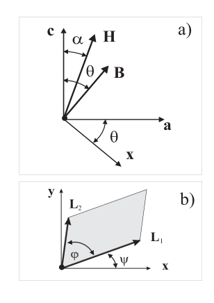
FIG. 1.: Definition of coordinate system and VLL primitive unit cell. a) Relative orientations in the plane containing ${\bf H}$, the $c$-axis and the equilibrium induction ${\bf B}$. The x-axis is perpendicular to ${\bf B}$ and the $y$-axis is perpendicular to the plane ${\bf H}$-${\bf B}$, pointing inside. b) Generic VLL primitive unit cell in the $x-y$ plane.

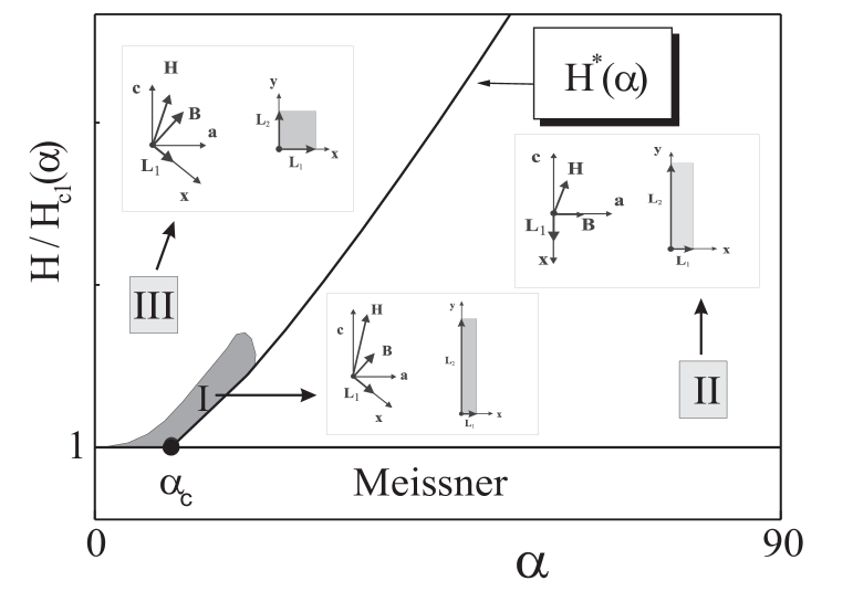
FIG. 2.: Generic phase diagram in the ($H,\alpha$) plane for both strong and moderate anisotropy.

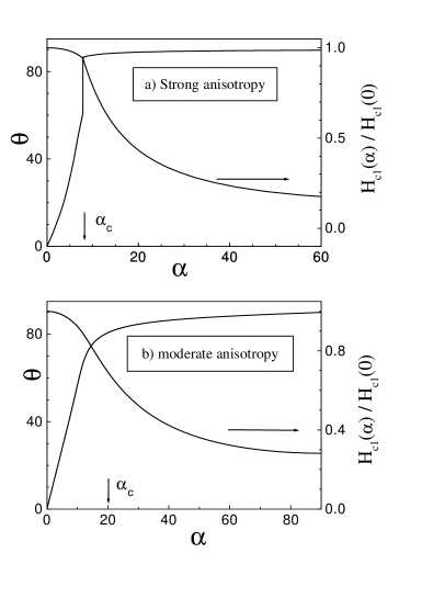
FIG. 3.: Results of Ref.[5] for $H_{c1}(\alpha)$ and $\theta$ vs. $\alpha$ for: a) strong anisotropy, b) moderate anisotropy

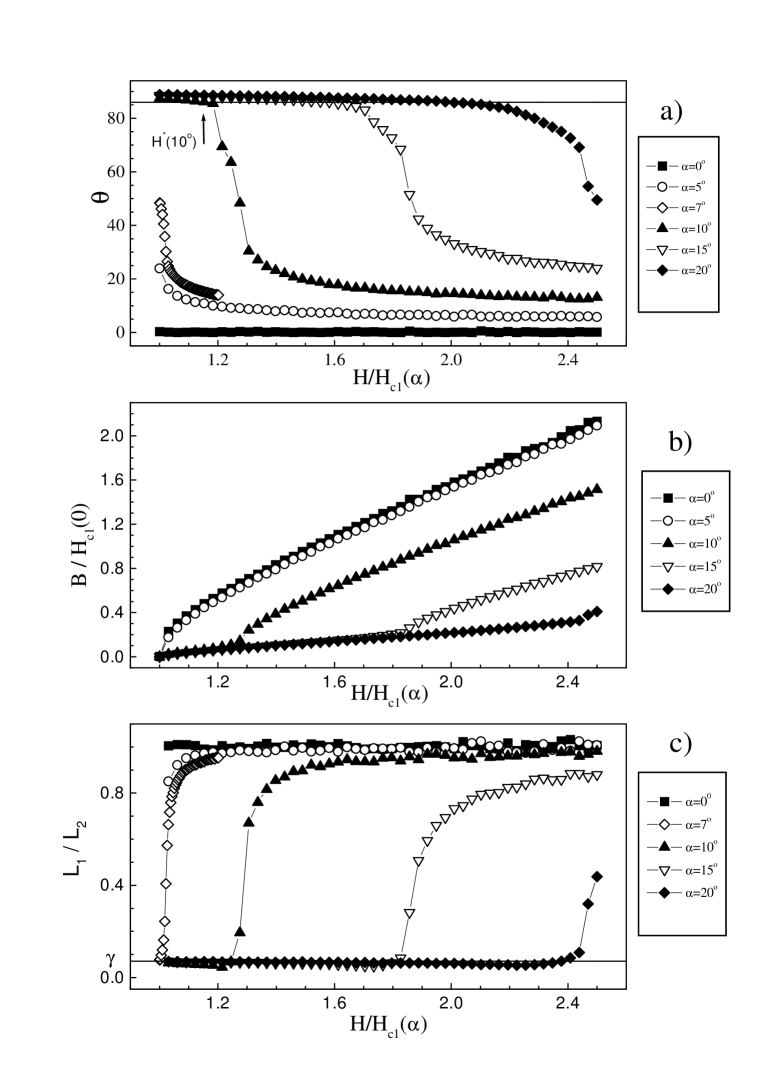
FIG. 4.: Numerical results for strong anisotropy. a) Vortex lines tilt angle. The full line $\theta=86^{o}$ corresponds to $\tan{\theta}=1/\gamma$. The arrow indicates $H^{*}(\alpha=10^{o}$). b) Magnetic induction. c) Ratio between VLL unit cell sides. The full line $\L_{1}/L_{2}=\gamma$ corresponds to the value predicted by scaling for $\alpha=90^{o}$

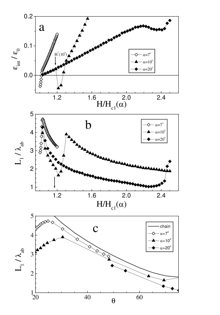
FIG. 5.: Numerical results for strong anisotropy. a) Interaction energy per vortex line. Arrow indicate the value of $H^{*}$ for $\alpha=10^{o}$. b) VLL period along x. c) VLL period along x vs. tilt angle compared with the period of an isolated vortex-line chain tilted at the same angle (full curve)

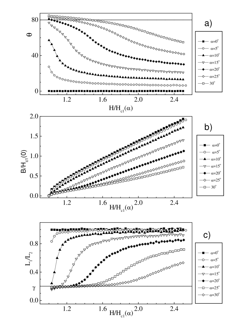
FIG. 6.: Numerical results for moderate anisotropy. a) Vortex lines tilt angle. The full line $\theta=80^{o}$ corresponds to $\tan{\theta}=1/\gamma$. b) Magnetic induction. c) Ratio between VLL unit cell sides. The full line $\L_{1}/L_{2}=\gamma$ corresponds to the value predicted by scaling for $\alpha=90^{o}$

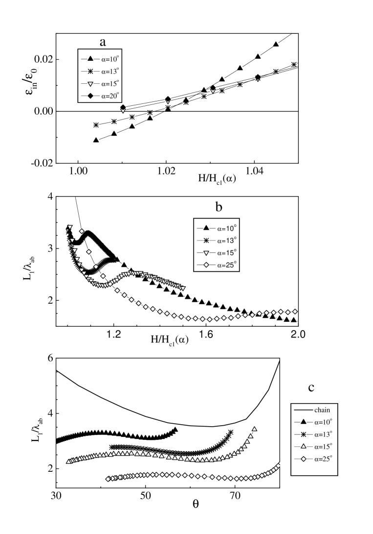
FIG. 7.: Numerical results for moderate anisotropy. a) Interaction energy per vortex line. b) VLL period along x. c) VLL period along x vs. tilt angle compared with the period of an isolated vortex-line chain tilted at the same angle (full curve)

REFERENCES

- [1] G. Blatter, M.V. Feigel’man,V.B. Geshkenbein, A.I. Larkin, and V.M. Vinokur, Rev. Mod. Phys. 66, (1994) 1125.
- [2] E.H. Brandt, Rep. Prog. Phys. 58, (1995) 1465.
- [3] L.J. Campbell, M.M. Doria and V.G. Kogan, Phys. Rev. B 38, (1988) 2439.
- [4] A.I. Buzdin, and A. Yu. Simonov, Physica C 175, (1991) 143.
- [5] A. Sudbø, E.H. Brandt, and D.A. Huse, Phys. Rev. Lett. 71, (1993) 1451.
- [6] W.A.M. Morgado, M.M. Doria and G. Carneiro, Physica C 349, (2001) 196.
- [7] A.M. Grishin, A.Yu. Martynovich, and S.V. Yampol’skii, Sov. Phys. JETP 70, (1990) 1089.
- [8] A.I. Buzdin, and A. Yu. Simonov, Physica C 168, (1990) 421.
- [9] V.G. Kogan, N. Nagakawam and S.L. Thiemann, Phys. Rev. B 42, (1990) 2631.
- [10] A.I. Buzdin, and S.S. Krotov, and D.A. Kuptsov, Physica C 175, (1990) 42.
- [11] A. Sudbø, and E.H. Brandt, Phys. Rev. Lett. 67, (1991) 3176.
- [12] R.A. Klemm and J.R. Clem, Phys. Rev. B 21, (1980) 1868.
- [13] M.M. Doria, Physica C. 178, (1991) 51.
- [14] W.A.M. Morgado and G.M. Carneiro, Physica C. 328, (1999) 195.