Jordan-Wigner approach to dynamic correlations in spin-ladders

Abstract

We present a method for studying the excitations of low-dimensional quantum spin systems based on the Jordan-Wigner transformation. Using an extended RPA-scheme we calculate the correlation function of neighboring spin flips which well approximates the optical conductivity of ${\rm Sr_{2}CuO_{3}}$. We extend this approach to the two-leg $S=\frac{1}{2}$–ladder by numbering the spin operators in a meander-like sequence. We obtain good agreement with the optical conductivity of the spin ladder compound (La,Ca)₁₄Cu₂₄O₄₁ for polarization along the rungs. For polarization along the legs higher order correlations are important to explain the weight of high-energy continuum excitations and we estimate the contribution of 4– and 6–fermion processes.

]

I Introduction

Due to the presence of strong quantum fluctuations, low-dimensional spin systems show very complex behavior and provide a challenge for theoretical treatments. In this context, S=$\frac{1}{2}$–Heisenberg spin ladders are especially interesting because they represent an interjacent system, in between the antiferromagnetic S=$\frac{1}{2}$–Heisenberg chain and the two-dimensional antiferromagnetic Heisenberg model. Early on, these spin ladders were considered as systems which display a dimensional crossover between one and two dimensions.[1] However, spin ladders do not constitute a “smooth crossover”, because even-leg spin ladders have a spin liquid ground state and finite spin gap. [2, 3] This is in contrast to the critical systems, the S=$\frac{1}{2}$–chain and the odd-leg ladders, which have algebraically decaying spin correlations and to the 2D antiferromagnetic Heisenberg model, for which a long-range Néel-ordered ground state was established. [4] In a field theoretical mapping of the low-energy modes on a O(3) nonlinear $\sigma$ model this even-odd effect in the number of legs results from the addition of a topological term. The term was demonstrated to be zero for even-leg ladders and the two-dimensional Heisenberg model and finite for odd-leg ladders as well as the S=$\frac{1}{2}$–chain.[5, 6, 7, 8] Correspondingly the system is gapless for odd-leg ladders and gapful for even-leg ladders whereby the gap decreases exponentially with the number of legs.

In this article we will focus on the antiferromagnetic two-leg S=$\frac{1}{2}$-ladders. The two-leg ladder can be approached conceptionally from the limit of strong coupling $J_{\perp}$ along the rungs. [9, 10, 11, 12] Then the elementary excitations can be considered as excitations of rung-triplets which propagate throughout the ladder due to the finite leg coupling $J$. For small coupling $J_{\perp}/J$, a more natural description would seem to be in terms of the spinon excitations of the isolated legs. However, the excitations of the two-leg spin-ladders cannot be constructed perturbatively from spinons of the chains since the rung coupling is a relevant perturbation. The spinons are confined and have to form bound states in the ladder-case. [13, 14]

Of particular interest is the intermediate coupling regime $J\approx J_{\perp}$, as this case is related to the two-dimensional systems. It is also realized in cuprate spin ladder compounds, [15, 16, 17] which are of interest due to their affinity to the cuprate high-$T_{c}$-superconductors. This intermediate regime is difficult to obtain and requires tedious calculations.

Here we propose an alternative approach, which is based on the Jordan-Wigner transformation [18, 19] and which is fairly simple. In contrast to previous applications of the Jordan-Wigner transformation to spin ladders by Dai and Su [20] and Azzouz et al. [21] we do not treat the phase factor within a mean-field or a flux-phase approximation. Rather we expand the phase factor and treat the resulting interaction terms on the same footing as the Ising term, which corresponds to a 4-fermion term in the Jordan-Wigner representation. We also apply this approach to the calculation of dynamic correlation functions. In particular we discuss the optical conductivity $\sigma(\omega)$, as it provides valuable information about high-energy $S$=0–spin excitations. In $\sigma(\omega)$ magnetic excitations can be observed due to the simultaneous excitation of a phonon, which breaks the inversion symmetry between two neighboring spins. The mechanism, which has been suggested by Lorenzana and Sawatzky, [22] provides a finite dipole moment to a simultaneous flip of neighboring spins. Since the phonon can take arbitrary momentum in this process, the magnetic $S$=0–excitations have to be averaged over the whole Brillouin zone to ensure zero total momentum. This mechanism has recently been used to investigate the high-energy spin excitations in the spin-ladder compound (La,Ca)₁₄Cu₂₄O₄₁ by Windt et al. [16] Using a perturbative approach, based on a continuous-unitary-transformation [23] and a Jordan-Wigner representation it was possible to identify the $S$=0–bound state of two triplets in the optical conductivity of (La,Ca)₁₄Cu₂₄O₄₁.

Here, we discuss in more detail the Jordan-Wigner approach which we have previously used in Ref. [16]. We introduce our approximation scheme for the Jordan-Wigner fermions for the simpler case of a 1d spin-chain in Sec. II. We calculate $\sigma(\omega)$ for the 1d-spin chain in RPA and compare with the optical conductivity of ${\rm Sr_{2}CuO_{3}}$ measured by Suzuura et al. [24] In Sec. III we generalize our Jordan-Wigner treatment to two-leg ladders by arranging the spins in a meander-like sequence. The mean field treatment of this representation, which is based on the expansion of all phase factors, is discussed in Sec. III A and the RPA-treatment in Sec. III B. We calculate dynamic spin-flip correlation functions in Sec. III C and compare $\sigma(\omega)$ for the two-leg ladder with the optical conductivity of (La,Ca)₁₄Cu₂₄O₄₁ in Sec. III D. The weight of processes involving the excitation of more than two fermions is estimated in Sec. III E. In Appendix A it is shown that our mean field treatment reproduces the correct strong coupling limit, in Appendix B the full set of RPA-equations for the two-leg ladder is listed. In Appendix C the role of the phase factor is explored, and in Appendix D the consequences of the artificial symmetry breaking introduced by our mean field treatment are discussed.

II Jordan-Wigner transformation for the 1d spin chain

First we recall the Jordan-Wigner transformation for the 1d spin chain and introduce our approximation scheme. The fact, that we find fairly good agreement with the spinon evaluation for the 1d spin-chain, inspired us to extend the approach to two-leg spin-ladders in Section III.

As spin operators do not obey canonical commutation relations, they are often transformed into either bosonic or fermionic operators, in order to permit the application of standard diagrammatic perturbation theory. With any mapping, however, the algebra of the original spin operators has to be preserved. For the Jordan-Wigner transformation this is provided by rewriting the spin operators as fermionic operators with a long-ranged phase factor

$$S_{i}^{-}=c_{i}e^{i\phi_{i}}\,,\,\,\phi_{i}=\pi\sum_{j<i}c_{j}^{\dagger}c_{j}\,,\,\,S_{i}^{z}=(c_{i}^{\dagger}c_{i}-\textrm{{\hbox{\frac{1}{2}}}})\,.$$ (1)

The representation is particularly useful for models with nearest-neighbor exchange interactions because in products of neighboring spins the phase factors drop out. This is due to the fact that the fermion operator $c_{i}$ commutes with the phase $\phi_{i}$ of the same site ($[c_{i},\phi_{i}]=0$) . Therefore the 1d antiferromagnetic Heisenberg Hamiltonian transforms to

$$H = J\sum_{i}\left\{\frac{1}{2}\left(c_{i}^{\dagger}c_{i+1}+c_{i+1}^{\dagger}c_{i}\right)\right.$$ (3)

$$\qquad\quad+\left.\left(c_{i}^{\dagger}c_{i}-\frac{1}{2}\right)\left(c_{i+1}^{\dagger}c_{i+1}-\frac{1}{2}\right)\right\}\,.$$

The first term in Eq. (3) corresponds to the XY-part of the original Heisenberg Hamiltonian. In the fermionic representation it acts as a nearest neighbor hopping. The second term, which originates from the Ising term of the original Heisenberg Hamiltonian, introduces a nearest neighbor density-density interaction among the fermions.

A Mean field treatment – d=1

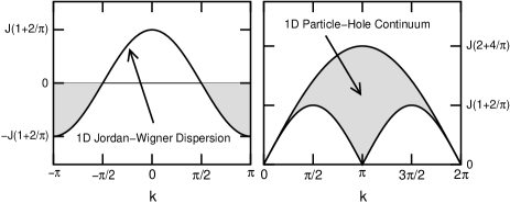
FIG. 1.: Left panel: mean field dispersion for the Jordan-Wigner fermions in $d$=1, grey shading denotes the filling in the ground state. Right panel: continuum of Jordan-Wigner particle-hole excitations in $d$=1.

Following Wang [25], the Ising-interaction can be treated in mean field approximation (MFA) by introducing a nearest neighbor “covalent bonding” of the Jordan-Wigner fermions $\chi=\langle c_{i}^{\dagger}c_{i+1}\rangle$.

$$H_{MF}=J\sum_{k}(1-2\chi)\cos k\,c_{k}^{\dagger}c_{k}\quad\textrm{with}\quad\chi=-\frac{1}{\pi}$$ (4)

The ground state of the Heisenberg model has no net magnetization $\langle S_{i}^{z}\rangle=0$. Within the fermionic representation this implies that the fermion system is at half filling $\langle c_{i}^{\dagger}c_{i}\rangle=\frac{1}{2}$. The ground state is obtained by filling up all negative energy states. This leads to a Fermi surface at wave vectors $k_{f}=\pm\frac{\pi}{2}$, as displayed in Fig. 1. Adding/removing a fermion to the system corresponds to $S_{z}=\pm 1$–excitations, $S_{z}=0$–excitations can be realized by particle-hole excitations. The particle-hole continuum of the Jordan-Wigner fermions, displayed in Fig. 1, is very similar to the two-spinon continuum [26]. The upper cutoff of the Jordan-Wigner particle-hole continuum is at $(2+\frac{4}{\pi})J\approx 3.27J$ and therefore close to $\pi J$ which is the maximum energy for two spinons.

B RPA for optical conductivity – d=1

High-energy spin excitations can be observed in the mid-infrared range of the optical conductivity $\sigma(\omega)$ due to the simultaneous excitation of a phonon. [22] The optical conductivity of the 1d spin-chain compound ${\rm Sr_{2}CuO_{3}}$ [24] has been nearly perfectly reproduced by Lorenzana and Eder [27] using an ansatz based on numerical results in finite chains, sum rules and Bethe ansatz results. Originally, a similar procedure was suggested by Müller et al.[28] for the evaluation of the dynamic structure factor $S(k,\omega)$, taking advantage of the observation that the two-spinon contribution is the class of Bethe-ansatz solutions which carries most of the weight of the continuum excitations. Only recently, it has been possible to determine the two-spinon contribution to $S(k,\omega)$ exactly.[29, 30]

For the optical conductivity, however, an exact expression of the two-spinon contribution is not yet available. Nevertheless, the evaluation of Lorenzana and Eder, [27] which nearly perfectly reproduces the shape of the cusp-like, wide structure in $\sigma(\omega)$, confirms that the observed resonance indeed results from two-spinon excitations of the nearest-neighbor Heisenberg model. This motivated us to use the established $\sigma(\omega)$ of the 1d spin-chain as a reference and check for the quality of the results of our analytical Jordan-Wigner approach. We calculate the two-particle correlation function $\sigma(\omega)$ within an extended RPA-scheme, i.e., by summing up bubble- and ladder-diagrams and compare our result with the experimental optical conductivity of ${\rm Sr_{2}CuO_{3}}$. [24]

For the one-dimensional spin-chain the phonon-assisted magnetic contribution to the optical conductivity is given by [22, 27]

$$\sigma(\omega)\sim-16\,\omega\sum_{p}\sin^{4}(\frac{p}{2}){\rm Im}\langle\langle\delta B_{-p};\delta B_{p}\rangle\rangle_{(\omega-\omega_{ph})}\,.$$ (5)

The spin-flip operator $\delta B_{p}$ is expressed in MFA by

$$\delta B_{p} =\frac{1}{N}\sum_{i}e^{ipr_{i}}\left({\bf S}_{i}{\bf S}_{i+1}-\langle{\bf S}_{i}{\bf S}_{i+1}\rangle\right)$$ (7)

$$\approx e^{-ip/2}\frac{1}{N}\sum_{k}(1-2\chi)\cos(k+\frac{p}{2})c_{k}^{\dagger}c_{k+p}\,.$$

This yields for the dynamic spin-flip correlation function in Zubarev notation

$$\langle\langle\delta B_{-p};\delta B_{p}\rangle\rangle = \frac{1}{N}\sum_{p}(1-2\chi)^{2}\left\{\cos^{2}\frac{p}{2}B^{(1,1)}(p,\omega)\right.$$ (8)

$$- \cos\frac{p}{2}\sin\frac{p}{2}\left(B^{(1,2)}(p,\omega)+B^{(2,1)}(p,\omega)\right)$$ (9)

$$+ \left.\sin^{2}\frac{p}{2}B^{(2,2)}(p,\omega)\right\}$$ (10)

with particle-hole propagators

$$B^{(\mu,\nu)}(p,\omega)=\sum_{k,q}f_{k}^{\mu}f_{q}^{\nu}\langle\langle c_{k}^{\dagger}c_{k+p};c_{q+p}^{\dagger}c_{q}\rangle\rangle$$ (11)

and the following form factors

$$f_{k}^{0}=1\,\,\,\,,\,\,\,\,f_{k}^{1}=\cos k\,\,\,\,,\,\,\,\,f_{k}^{2}=\sin k\,.$$ (12)

FIG. 2.: Diagrammatic scheme for the extended RPA treatment of Jordan-Wigner fermions in Eq. (15).

Summing all particle-hole scattering processes, as illustrated in Fig. 2 in diagrammatic terms, a simple expression for the renormalized particle-hole propagator can be obtained

$${\rm B}^{(\mu,\nu)}(p,\omega)={\rm b}^{(\mu,\nu)}(p,\omega) + 2J\cos p\,{\rm b}^{(\mu,0)}(p,\omega){\rm B}^{(0,\nu)}(p,\omega)$$ (13)

$$- 2J\,{\rm b}^{(\mu,1)}(p,\omega){\rm B}^{(1,\nu)}(p,\omega)$$ (14)

$$- 2J\,{\rm b}^{(\mu,2)}(p,\omega){\rm B}^{(2,\nu)}(p,\omega)\,,$$ (15)

where the noninteracting particle-hole propagators are given by

$${\rm b}^{(\mu,\nu)}(p,\omega) = \frac{1}{N}\sum_{k}f_{k}^{\mu}f_{k}^{\nu}\left\{\frac{(1-\langle n_{k+p}\rangle)\langle n_{k}\rangle}{\omega+\epsilon_{k}-\epsilon_{p+k}+i0^{+}}\right.$$ (17)

$$\qquad\qquad\qquad-\left.\frac{(1-\langle n_{k}\rangle)\langle n_{p+k}\rangle}{\omega+\epsilon_{k}-\epsilon_{p+k}-i0^{+}}\right\}\,.$$

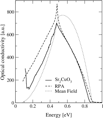
FIG. 3.: $\sigma(\omega)$ obtained with Jordan-Wigner fermions in comparison with the experimental optical conductivity of ${\rm Sr_{2}CuO_{3}}$ (solid line), taken from Suzuura et al. [24] Dotted line: mean-field approximation, dashed line: RPA-approximation. Following Lorenzana and Eder [27] we have subtracted the same linear background from the experimental data and we have used the same value for the exchange coupling $J$=0.246eV and for the phonon-frequency $\omega_{ph}$=0.08eV.

Evaluation of these equations determines $\sigma(\omega)$ which is shown in Fig. 3 in comparison with the experimental spectrum of ${\rm Sr_{2}CuO_{3}}$ taken from Suzuura et al. [24]

A simple analysis of the experimental line shape of ${\rm Sr_{2}CuO_{3}}$ based on Jordan-Wigner fermions has already been discussed by Suzuura et al. [24] in combination with the experimental results. However, they restricted the evaluation to the XY-model which corresponds to our mean field evaluation apart from a renormalization of the energy scale by a factor of $1+2/\pi$ in Eq. (4). We find that it is important to treat the two-particle correlation function $\sigma(\omega)$ at least within RPA. The resonance is shifted to lower energies compared to the mean field approximation. In addition we observe a cusp at $\omega=J(1+2/\pi)$ as a precursor of the logarithmic singularity found by Lorenzana and Eder. [27] Despite the good agreement with respect to the cusp and to the high energy side of the cusp, however, our RPA treatment seems to overestimate the effect of the interaction because too much spectral weight is shifted to energies below the cusp. This effect could possibly be compensated by consideration of higher order correlations.

III Jordan-Wigner Transformation for the two-leg $S=\frac{1}{2}$-ladder

Motivated by the results of our Jordan-Wigner fermion treatment for the Heisenberg $S=\frac{1}{2}$–chain we “slightly increase” the dimensionality and extend the approach to the nearest neighbor Heisenberg two-leg $S=\frac{1}{2}$–ladder:

$$H=J_{\perp}\!\sum_{i}{\bf S}_{i,1}{\bf S}_{i,2}\!+\!J\!\sum_{i}({\bf S}_{i,1}{\bf S}_{i+1,1}\!+{\bf S}_{i,2}{\bf S}_{i+1,2})\,,$$ (18)

where $J_{\perp}$ is the exchange coupling along the rungs, $J$ the coupling along the legs, $i$ refers to the site index along the legs and the subscripts $1,2$ label the two different legs.

Generalizations of the Jordan-Wigner transformation to higher dimensions have been suggested [31, 32] and may be adopted for spin ladders. For spin ladders the one-dimensional Jordan-Wigner transformation can be applied directly, when all spins are arranged in a one-dimensional sequence. With this scheme we can control the range of the interaction terms through a convenient choice of a path covering all sites, whereas the application of a two-dimensional representation to the spin ladders would generate long-range interaction terms in the Hamiltonian. Possible path configurations through a two-leg ladder are shown in Fig. 4.

FIG. 4.: Possible path configurations for a two-leg ladder.

The path displayed in Fig. 4(a) is obviously very close to the one-dimensional situation. As a consequence the rung interaction is difficult to treat in this representation because every product of neighboring rung-spins contains an infinite number of phase-factors. The rung-coupling, however, is a relevant perturbation since the excitation spectrum of a two-leg ladder remains gapped for all coupling ratios $J_{\perp}/J$. Therefore a path which passes through all the rungs should be more suitable. Possible realizations are a zigzag path[21] and a meander path[20], displayed in Fig. 4(b) and (c), respectively. Although the zigzag path appears simpler and more symmetric at first sight, we show in Appendix A that within a mean field treatment (analogous to the previous section) only the meander path can reproduce the correct strong coupling limit of the one-triplet dispersion $\epsilon_{k}=J_{\perp}+J\cos k$ for $J_{\perp}/J\gg 1$. Therefore we chose the meander path even though the nearest neighbor Heisenberg-Hamiltonian is slightly more complicated in this representation.

Following Dai and Su [20] we divide the ladder into two sublattices as indicated in Fig. 5. Introducing two species of spinless fermions $\alpha_{i}$ and $\beta_{i}$, the spin operators on the two sublattices transform as:

$$S_{i,\alpha}^{+} = \alpha_{i}^{\dagger}e^{i\pi\sum_{j<i}(\alpha_{j}^{\dagger}\alpha_{j}+\beta_{j}^{\dagger}\beta_{j})}$$ (19)

$$S_{i,\beta}^{+} = \beta_{i}^{\dagger}e^{i\pi\sum_{j<i}(\alpha_{j}^{\dagger}\alpha_{j}+\beta_{j}^{\dagger}\beta_{j})}e^{i\pi\alpha_{i}^{\dagger}\alpha_{i}}\,,$$ (20)

where the summation in the phase factor is along the meander path. For products of spin operators, which are not successive along the meander path, like e.g. $S_{i,\alpha}^{+}S_{i+1,\beta}^{-}+S_{i,\alpha}^{-}S_{i+1,\beta}^{+}$, the phases corresponding to intermediate sites along the meander path do not cancel. This is different from the one-dimensional situation where all nearest-neighbor spin operators are also successive along the path. Using transformation (19) the Heisenberg Hamiltonian of Eq. (18) becomes:

$$H= J_{\perp} \sum_{i}\left\{\frac{1}{2}(\alpha_{i}^{\dagger}\beta_{i}+\beta_{i}^{\dagger}\alpha_{i})+(\alpha_{i}^{\dagger}\alpha_{i}-\frac{1}{2})(\beta_{i}^{\dagger}\beta_{i}-\frac{1}{2})\right\}$$ (21)

$$+ J \sum_{i}\left\{\,\frac{1}{2}\left[\beta_{i}^{\dagger}\alpha_{i+1}+\alpha_{i}^{\dagger}\beta_{i+1}e^{i\pi(n_{\beta_{i}}+n_{\alpha_{i+1}})}+{\rm H.c.}\right]\right.$$ (24)

$$\qquad\quad+\,(\alpha_{i}^{\dagger}\alpha_{i}-\frac{1}{2})(\beta_{i+1}^{\dagger}\beta_{i+1}-\frac{1}{2})$$

$$\left.\qquad\quad+\,(\alpha_{i+1}^{\dagger}\alpha_{i+1}-\frac{1}{2})(\beta_{i}^{\dagger}\beta_{i}-\frac{1}{2})\right\}\,.$$

Unfortunately the phase factor $e^{i\pi(n_{\beta_{i}}+n_{\alpha_{i+1}})}$ from spin products of non-successive sites cannot be treated exactly. Dai and Su have replaced this phase factor by its average value. This treatment, however, can be improved in a systematic way by expanding the phase factor:

$$e^{i\pi(n_{\beta_{i}}+n_{\alpha_{i+1}})}=(1-2\beta_{i}^{\dagger}\beta_{i})(1-2\alpha_{i+1}^{\dagger}\alpha_{i+1})$$ (25)

and reinserting this expansion into Hamiltonian (21). In this way we obtain additional interaction terms containing 4– and 6–fermion operators which we now treat on the same footing as the Ising-interaction terms.

FIG. 5.: Sublattice structure for the meander path.

A Mean field treatment – Ladder

Inspired by the results of the mean-field treatment for the spin chain, we adopt a similar approach here and consider all possible nearest-neighbor bond amplitudes:

$$\chi_{0}=\langle\beta_{i}^{\dagger}\alpha_{i}\rangle\,\,\,,\,\,\,\chi_{1}=\langle\beta_{i}^{\dagger}\alpha_{i+1}\rangle\,\,\,,\,\,\,\chi_{2}=\langle\alpha_{i}^{\dagger}\beta_{i+1}\rangle\,.$$ (26)

Taking into account all possible contractions of the 4- and 6-fermion operator terms we arrive at the following mean-field Hamiltonian:

$$H_{MF}=\sum_{k}(\gamma_{k}\alpha_{k}^{\dagger}\beta_{k}+H.c.)$$ (27)

with

$$\gamma_{k} = J_{\perp}(\frac{1}{2}-\chi_{0})+4J\chi_{0}\chi_{1}$$ (30)

$$+\,\,J\cos k(\frac{1}{2}+2\chi_{0}^{2}-4\chi_{1}\chi_{2}-\chi_{1}-\chi_{2}-2\chi_{1}^{2})$$

$$+\,\,iJ\sin k(\frac{1}{2}+2\chi_{0}^{2}-4\chi_{1}\chi_{2}-\chi_{1}+\chi_{2}+2\chi_{1}^{2})\,.$$

This expression has already been simplified using that $\chi_{0}$, $\chi_{1}$ and $\chi_{2}$ turn out to be real. The above Hamiltonian can easily be diagonalized

$$H_{MF}=\sum_{k}\epsilon_{k}(\tilde{\alpha}_{k}^{\dagger}\tilde{\alpha}_{k}-\tilde{\beta}_{k}^{\dagger}\tilde{\beta}_{k})\quad\textrm{with}\quad\epsilon_{k}=|\gamma_{k}|$$ (31)

using

$$\alpha_{k}=\frac{1}{\sqrt{2}}u_{k}(\tilde{\alpha}_{k}+\tilde{\beta}_{k})\quad \quad\beta_{k}=\frac{1}{\sqrt{2}}v_{k}(\tilde{\alpha}_{k}-\tilde{\beta}_{k})$$ , (32)

$$\qquad u_{k}=v_{k}^{*}=e^{i\phi_{k}/2}\quad \quad\gamma_{k}=|\gamma_{k}|e^{i\phi_{k}}\,.$$ , (33)

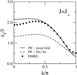
FIG. 6.: Dispersion for the isotropic ladder $J=J_{\perp}$. Solid line: mean field dispersion for Jordan-Wigner fermions; dashed line: dispersion obtained by averaging the phase factor analogous to the treatment by Dai and Su;[20] circles: one-triplet dispersion obtained with DMRG for a $N$=80–site ladder.[17]

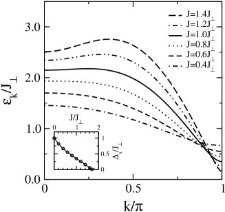
FIG. 7.: Mean-field dispersion for Jordan-Wigner fermions for different coupling ratios $J/J_{\perp}$. Inset: spin gap $\Delta_{s}$ as a function of $J/J_{\perp}$.

For the isotropic ladder, i.e. $J=J_{\perp}$, we obtain $\chi_{0}=-0.3617$, $\chi_{1}=-0.2679$ and $\chi_{2}=0.1777$. As the product of the bond amplitudes around a plaquette is negative, our mean field treatment corresponds to a $\pi$-flux state of the spinless fermions. Note, that this $\pi$-flux phase is different from that of Azzouz et al., [21] who have by construction replaced the complete phase factor by a $\pi$-flux phase. Both approaches are compared in Appendix C.

The resulting dispersion is displayed in Fig. 6, in comparison with the dispersion for a $N$=80-site ladder obtained by DMRG.[17] For momenta between $k\approx 0.5\pi$–$0.9\pi$ we find nearly perfect agreement with the DMRG results. The spin gap at $k=\pi$, however, is too small and for momenta $k<\pi/2$ the energy is overestimated. Nevertheless, our mean-field treatment is able to reproduce a dip for small momenta, which is a precursor of the symmetric (with respect to $k=\pi/2$) spinon dispersion of the spin chain. The dip becomes more pronounced when the leg coupling $J/J_{\perp}$ is increased as can be seen in Fig. 7. Note that within a mean-field treatment of the bosonic bond-operator representation of elementary rung-triplets [10, 11] it has not been possible to achieve a dispersion-dip for the isotropic ladder.

To demonstrate the improvement of our mean-field evaluation with respect to the mean-field treatment by Dai and Su, [20] who have replaced the phase factor by its expectation value, we have added their dispersion in Fig. 6. Qualitatively it is very similar to our mean-field dispersion. Its magnitude, however, is by a factor of about 1.5 too small over a large part of the Brillouin zone. Therefore we conclude that an adequate treatment of the phase factor is very important and it is necessary to go beyond averaging of the phase factor.

The spin gap $\Delta_{s}$, which is shown in the inset of Fig. 7 as a function of $J/J_{\perp}$, is underestimated by our approach. It even vanishes for $J\approx 1.7J_{\perp}$. As the spin gap is known to be finite for all finite $J/J_{\perp}$, this coupling ratio marks the breakdown of our mean field treatment.

B Extended RPA-treatment – Ladder

The optical conductivity $\sigma(\omega)$ constitutes a powerful probe of the spin excitations of a spin ladder. It has been possible to verify experimentally the existence of a $S$=0–two triplet bound state in the optical conductivity of the spin ladder compound (La,Ca)₁₄Cu₂₄O₄₁[16] and a more refined analysis has shown that it is necessary to include a 4-spin cyclic exchange interaction [17] of about $J_{cyc}\approx 0.20-0.27J_{\perp}$. Bound states in the singlet and triplet excitation channel were predicted by Sushkov and Kotov [11] and by Damle and Sachdev,[33] similar to the states analyzed by Uhrig and Schulz [34] in dimerized spin chains. More extensive perturbative investigations, within a linked cluster expansion, were performed by Trebst et al. [12] and the observability of the singlet bound state was suggested by Jurecka and Brenig[35].

Here, we will demonstrate, how the spin-flip correlation functions, which contribute to $\sigma(\omega)$, can be obtained within the Jordan-Wigner approach. We discuss the resultant correlation functions for an isotropic ladder $J=J_{\perp}$, without cyclic exchange ($J_{cyc}=0$), and focus on the $S$=0–bound state and the continuum excitations. For the calculation of the optical conductivity we will concentrate on an isolated ${\rm Cu_{2}O_{3}}$-ladder. The phonon-assisted magnetic contribution to $\sigma(\omega)$ results largely from the simultaneous excitation of two neighboring spin-flips plus a Cu-O bond-stretching phonon:

$$\sigma(\omega)\sim-\omega\sum_{p}\sum_{p_{y}=0,\pi}f_{p}\,{\rm Im}\langle\langle\delta B_{-{\bf p}};\delta B_{\bf p}\rangle\rangle_{(\omega-\omega_{ph})}$$ (34)

where ${\bf p}=(p,p_{y})$ and the operators

$$\delta B_{\bf p}^{\rm leg} = \frac{1}{N}\!\sum_{i}\!\sum_{l=1\!,2}e^{i{\bf p}{\bf r}_{i\!,l}}\!\left({\bf S}_{i,l}{\bf S}_{i+1\!,l}\!-\!\langle{\bf S}_{i,l}{\bf S}_{i+1\!,l}\rangle\right)$$ (35)

$$\delta B_{\bf p}^{\rm rung} = \frac{1}{N}\sum_{i}e^{i{\bf p}{\bf r}_{i}}\left({\bf S}_{i,1}{\bf S}_{i,2}-\langle{\bf S}_{i,1}{\bf S}_{i,2}\rangle\right)$$ (36)

are the spin-flip operators for polarization of the electrical field along the legs and the rungs, respectively.

Following our previous treatment in Ref. [17], we consider phonon form factors given by:

$$f_{p}^{\rm leg}=8\sin^{4}(\frac{p}{2})\,\,\,\,,\,\,\,\,f_{p}^{\rm rung}=8\sin^{2}(\frac{p}{2})+4\,.$$ (37)

Here, $f_{p}^{\rm leg}$ originates from the coupling to in-phase and out-of-phase stretching modes of O-ions on the legs and is the same form factor as for an isolated spin chain. For $f_{p}^{\rm rung}$ we take in addition to the out-of-phase stretching mode also the vibration of the O-ion on the rung into account, which is responsible for the constant contribution in Eq. (37).

For the calculation of the spin-flip correlation function we apply the Jordan-Wigner transformation (19) to the spin-flip operators ${\bf S}_{i,1}{\bf S}_{i+1,1}\pm{\bf S}_{i,2}{\bf S}_{i+1,2}$ and ${\bf S}_{i,1}{\bf S}_{i,2}$. All terms with 4 and 6 fermion operators are reduced to two-operator terms by replacing all surplus operators with their contractions (26). With this procedure the Fourier transform of the spin-flip operators becomes:

$$\delta B_{p}^{\rm rung} = \frac{1}{\sqrt{N}}\sum_{k}(\frac{1}{2}-\chi_{0})\left(\alpha_{k}^{\dagger}\beta_{p+k}+\beta_{k}^{\dagger}\alpha_{p+k}\right)$$ (38)

$$\delta B_{p,p_{y}=0}^{\rm leg} = \frac{1}{\sqrt{N}}\sum_{k}\left\{\alpha_{k}^{\dagger}\beta_{p+k}(a+be^{ik}-ce^{-i(p+k)})\right.$$ (40)

$$\qquad\quad\,\,+\left.\beta_{k}^{\dagger}\alpha_{p+k}(a+be^{-i(p+k)}-ce^{ik})\right\}$$

$$\delta B_{p,p_{y}=\pi}^{\rm leg} = \frac{1}{\sqrt{N}}\sum_{k}\left\{\alpha_{k}^{\dagger}\beta_{p+k+\pi}(-a+\tilde{b}e^{ik}-ce^{-i(p+k)})\right.$$ (42)

$$\qquad\quad\,\,+\left.\beta_{k}^{\dagger}\alpha_{p+k+\pi}(-a-\tilde{b}e^{-i(p+k)}+ce^{ik})\right\}$$

with

$$a=4\chi_{0}\chi_{1}\,\,,\,\,b=\frac{1}{2}+2\chi_{0}^{2}-4\chi_{1}\chi_{2}-\chi_{1}$$ (43)

$$c=2\chi_{1}^{2}+\chi_{2}\,\,,\,\,\tilde{b}=\frac{1}{2}-2\chi_{0}^{2}+4\chi_{1}\chi_{2}-\chi_{1}\,.$$ (44)

Inserting the spin-flip operators (38) into the optical conductivity (34) produces a sum of particle-hole propagators with different form factors. To evaluate these particle-hole propagators in RPA we prefer to use the original fermionic operators $\alpha,\beta$ because transformation to the operators $\tilde{\alpha},\tilde{\beta}$ (32) would increase the number of interaction terms considerably.

Prior to the derivation of the RPA-equations, the interaction terms in the Hamiltonian have to be reduced to two-particle interactions in order to deal only with 4–particle vertices. Accordingly, all 6–operator terms, which appear in Eq. (21), are reduced to 4–operator terms by replacing all possible contractions with the corresponding bond amplitudes (26). In this way, we obtain the following reduced interaction term from Hamiltonian (21):

$$H_{\rm red} =J\frac{1}{N}\sum_{k_{1}...k_{4}}\delta(k_{1}+k_{2}-k_{3}-k_{4})$$ (50)

$$\!\!\!\!\!\!\!\left\{\alpha_{k_{1}}^{\dagger}\beta_{k_{2}}^{\dagger}\beta_{k_{3}}\alpha_{k_{4}}\left[\frac{J_{\perp}}{J}+e^{i(k_{2}-k_{3})}+(1+4\chi_{2})e^{-i(k_{2}-k_{3})}\right.\right.$$

$$\qquad\qquad\qquad\qquad\!+\,2\chi_{1}(e^{i(k_{1}+k_{2})}+e^{-i(k_{1}+k_{2})})$$

$$\qquad\qquad\qquad\qquad\!\left.-\,2\chi_{0}(e^{ik_{1}}+e^{-ik_{2}}+e^{ik_{3}}+e^{-ik_{4}})\right]$$

$$\!\!\!\!\!\!\!+\,\alpha_{k_{1}}^{\dagger}\alpha_{k_{2}}^{\dagger}\beta_{k_{3}}\beta_{k_{4}}\,\,2\chi_{1}e^{i(k_{2}-k_{3})}$$

$$\!\!\!\!\!\!\!\left.+\,\beta_{k_{1}}^{\dagger}\beta_{k_{2}}^{\dagger}\alpha_{k_{3}}\alpha_{k_{4}}\,\,2\chi_{1}e^{i(k_{1}-k_{4})}\right\}$$

A set of RPA-equations for the particle-hole propagators, which are listed in Appendix B, can be obtained by consideration of all possible vertex-configurations of the interaction Hamiltonian (50). In real space these vertices correspond not only to a summation of bubble-diagrams, but also include ladder-diagrams and other non-local terms as indicated in Fig. 8. For this reason we use the term extended RPA-treatment.

FIG. 8.: Diagrammatic representation of the processes which contribute to the extended RPA-treatment, in real space.

C Spin-flip correlation functions

We have calculated the correlation functions for spin-flips along the legs $\delta B_{p,p_{y}=0}^{\rm leg}$, $\delta B_{p,p_{y}=\pi}^{\rm leg}$ and for spin-flips along the rungs $\delta B_{p}^{\rm rung}$ for an isotropic ladder $J=J_{\perp}$ using the RPA-treatment of the previous section. The results are presented in Figs. 9, 11 and 12, respectively. For comparison the mean-field evaluation of each of the correlation functions is displayed in the lower panels.

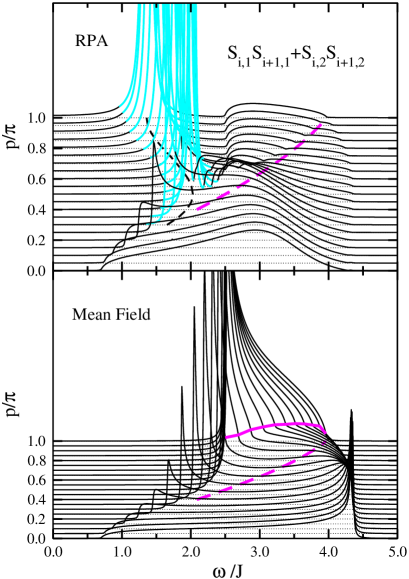
FIG. 9.: RPA and mean-field evaluation of the momentum resolved correlation function $\langle\langle\delta B_{-p,p_{y}=0}^{\rm leg};\delta B_{p,p_{y}=0}^{\rm leg}\rangle\rangle$, where a broadening of $\delta=0.01J$ has been used. The grey lines (upper panel) designate the $S$=0-bound state. The dashed dark grey line is a projection of the dark grey line in the lower panel, which links the points of sharp increase in the middle of the continuum. This is a precursor of the upper edge of the 2-spinon continuum in single chains. [23, 36] In RPA a dip structure remains at the same position in the continuum.

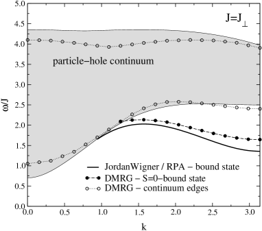
FIG. 10.: Particle–hole continuum of the Jordan–Wigner fermions and $S$=0–bound state (thick solid line) in comparison with the two-triplet continuum (open symbols) and $S$=0–bound state (filled symbols) obtained by DMRG for a ladder with $N$=80–sites.[17]

In the mean-field evaluation of $\langle\langle\delta B_{-p,p_{y}=0}^{\rm leg};\delta B_{p,p_{y}=0}^{\rm leg}\rangle\rangle$ (lower panel of Fig. 9) one observes van-Hove singularities at the upper edge of the continuum for small momenta and at the lower edge of the continuum for large momenta. With the RPA-treatment the van-Hove singularities at the continuum edges disappear. For small momenta the maximum of the continuum is shifted from the upper edge downwards to about $\omega\approx 3J$. At large momenta we see the formation of the $S$=0-bound state. The bound state emerges from the continuum at approximately $k\approx 0.3\pi$, it passes through a maximum at $k\approx\pi/2$ and a minimum at $k=\pi$. In Fig. 10 the dispersion of the bound state is compared with the DMRG calculation for a $N$=80–site ladder. [17] We find good agreement between both methods, only the energy of the RPA-dispersion is slightly too low. This indicates that the interaction strength is somewhat overestimated in RPA.

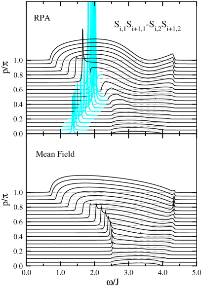
FIG. 11.: RPA and Mean-field evaluation of the correlation function $\langle\langle\delta B_{-p,p_{y}=\pi}^{\rm leg};\delta B_{p,p_{y}=\pi}^{\rm leg}\rangle\rangle$, where a broadening of $\delta=0.01J$ has been used. The grey lines indicate the $S$=0-bound state.

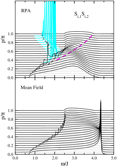
FIG. 12.: RPA and Mean-field evaluation of the correlation function $\langle\langle\delta B_{-p}^{\rm rung};\delta B_{p}^{\rm rung}\rangle\rangle$, where a broadening of $\delta=0.01J$ has been used. The grey lines indicate the $S$=0-bound state. The dashed dark grey line in the upper panel is the same as in Fig. 9.

In the mean field evaluation of the out-of-phase component of the correlation function for spin-flips along the legs $\langle\langle\delta B_{-p,p_{y}=\pi}^{\rm leg};\delta B_{p,p_{y}=\pi}^{\rm leg}\rangle\rangle$ (lower panel in Fig. 11) the van–Hove singularities at the continuum edges are suppressed. The overall momentum dependence on $p$ appears to be reversed when the out-of-phase component in Fig. 11 (upper panel) is compared to the in-phase component in Fig. 9 (upper panel). This is caused by the checker-board sublattice structure of the meander path, which shifts the momentum of the particle-hole propagator $\delta B_{p,p_{y}=\pi}^{\rm leg}$ by $\pi$ in relation (38). The inversion of the momentum dependence is especially noticeable for the bound state. However, the out-of-phase component should not contain the bound state at all but only contribute to the continuum excitations, an issue that we have addressed previously in Ref. [17]. The argument is based on the observation that the out-of-phase component originates from the excitation of 3 different rung-triplets, [17] when it is expressed in terms of rung-triplet operators. [9, 10] The $S$=0–bound state, on the other hand, arises from scattering processes of two equal triplets and therefore cannot be present in the out–of–phase component. Although the spectral weight of the bound state in the $p_{y}=\pi$ component is only small, this indicates a failure of our approach. This failure is probably related to the fact that the meander path breaks certain symmetries of the original ladder model. In our mean-field evaluation we find, e.g., $\langle{\bf S}_{i,1}{\bf S}_{i+1,1}\rangle\neq\langle{\bf S}_{i,2}{\bf S}_{i+1,2\rangle}$. This artificial symmetry breaking will be discussed in more detail in Appendix D. However, the resultant effects may average out to some extent in the sum of the spin-flip operators on both legs ${\bf S}_{i,1}{\bf S}_{i+1,1}+{\bf S}_{i,2}{\bf S}_{i+1,2}$, whereas they will probably even be enhanced in the difference ${\bf S}_{i,1}{\bf S}_{i+1,1}-{\bf S}_{i,2}{\bf S}_{i+1,2}$. This may explain the shortcomings of our approach with respect to the out-of-phase component, while we find reasonable results for the in-phase-component.

In Fig. 12 the RPA- and mean-field evaluation for the correlation function of spin-flips along the rungs $\langle\langle\delta B_{-p}^{\rm rung};\delta B_{p}^{\rm rung}\rangle\rangle$ are shown in the upper and lower panel, respectively. For $p=0$ it is identical to the $p=0$–component of the in-phase correlation function for spin-flips along the legs $\langle\langle\delta B_{-p,p_{y}=0}^{\rm leg};\delta B_{p,p_{y}=0}^{\rm leg}\rangle\rangle$ and both correspond to the correlation function for the Raman response. [37, 38] For larger momenta, the spectral weight of the rung-correlation is much smaller than the in-phase component of the leg-correlations and at $p=\pi$ the weight of the $S$=0 bound state vanishes according to a selection rule. [16]

D Optical conductivity

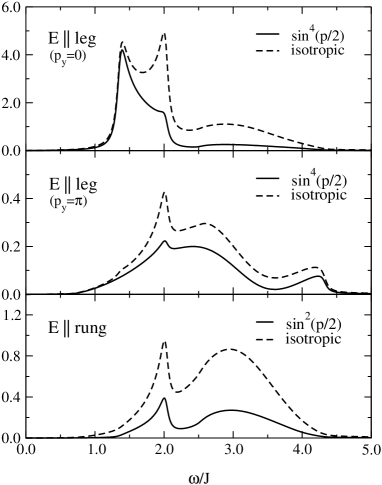
FIG. 13.: Momentum integrated spin–flip correlation functions, which contribute to $\sigma(\omega)$ for polarization along the legs (top and middle panel) and for polarization along the rungs (bottom panel). In order to visualize the resulting contribution to $\sigma(\omega)$ in Eq. (34) each correlation function has been multiplied with the frequency $\omega$ and for each of them the momentum integration without prefactor (dashed lines) and with the corresponding prefactors of Eq. (37) (solid lines) are shown.

Once the momentum dependent spin-flip correlation functions, shown in Figs. 9, 11 and 12, are known the optical conductivity $\sigma(\omega)$ in Eq. (34) can easily be obtained by integration. In Fig. 13 the momentum integrated spin-flip correlation functions are displayed whereby we present them with form factors equal to unity (dashed lines) and with the form factors of Eq. (37) (solid lines). To demonstrate their contribution to $\sigma(\omega)$, all spectra have already been multiplied with frequency $\omega$.

For polarization parallel to the legs and $p_{y}=0$ (top panel of Fig. 13) two dominant peaks appear at $\omega_{1}\approx 1.4J$ and $\omega_{2}\approx 2.0J$. They are caused by van Hove singularities arising from the dispersion of $S$=0–bound state [16] at $p=\pi$ and $p\approx\pi/2$. The upper peak at $\omega_{2}$ is suppressed by consideration of the relevant form factor $\sin^{4}(p/2)$. Also the continuum excitations are reduced considerably because they originate largely from small momenta, where no bound state is present, see Fig. 9. The out-of-phase component (middle panel of Fig. 13) is an order of magnitude smaller than the in-phase component. We consider the results for the out-of-phase component, however, less reliable due to symmetry breaking by the meander path, as mentioned in the previous section.

For polarization parallel to the rungs (bottom panel of Fig. 13) two form factors contribute to $\sigma(\omega)$, a constant and a $\sin^{2}(p/2)$–term. Only the upper bound state at $\omega_{2}$ is present in the momentum integrated spectrum because the $S$=0–bound state is suppressed at $p=\pi$ in accord with a selection rule, [16] see also Fig. 12.

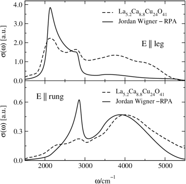
FIG. 14.: Comparison of the Jordan–Wigner spectra for the isotropic ladder using an exchange coupling of $J$=1100cm${}^{-}1$ with the experimental $\sigma(\omega)$ of ${\rm La_{5.2}Ca_{8.8}Cu_{24}O_{41}}$. The experimental spectra have been measured by Windt and Grüninger. [17] For the phonon a frequency of $\omega_{ph}$=600cm^-1 has been assumed for polarization along the legs and $\omega_{ph}$=650^-1 for polarization along the rungs.

In Fig. 14 our spectra are compared with the experimental optical conductivity of ${\rm La_{5.2}Ca_{8.8}Cu_{24}O_{41}}$ for polarization along the legs (top panel) and for polarization along the rungs (bottom panel). Following our previous treatment in Ref. [16], an exchange coupling of $J$=1100cm^-1, a phonon frequency of $\omega_{ph}$=600cm^-1 for polarization along the legs and $\omega_{ph}$=650cm^-1 for polarization along the rungs have been used. The difference of 50cm^-1 in the phonon frequencies for polarization along the legs and the rungs accounts for the shift observed experimentally with respect to the upper bound state in both polarizations. [16, 17]

For polarization along the legs we find good agreement with respect to the bound states. The continuum contribution, however, is strongly underestimated. To some extent this is due to the fact that, so far, we considered only the creation of two fermions at the external current vertex: we approximated the spin-flip operators in Eq. (38) by a particle-hole creation operator. Without this approximation the correlation functions $\langle\langle\delta B_{-p,p_{y}=0,\pi}^{\rm leg};\delta B_{p,p_{y}=0,\pi}^{\rm leg}\rangle\rangle$ would contain also the excitation of 4– and 6–fermions, which would increase the amount of high-energy excitations. The weight of these higher order excitations will be estimated in the next section.

For polarization parallel to the rungs we find very good agreement even with respect to the weight and line shape of the continuum. Rung correlations are obviously treated quite accurately in our meander-path representation. There are no phase factors in the product of two spin operators on the same rung because they are neighboring along the meander path. Therefore the only 4–fermion process results from the Ising-like term in the rung operator (35).

E Higher order contributions

The contribution of 4– and 6–fermions to the spin-flip correlation functions in leg polarization can be obtained analogous to the 2–fermion contribution. In the spin-flip operator $\delta B_{p}^{\rm leg}$, Eq. (35), the spin operators are replaced by fermionic operators. Terms with 6 operators are designated as the 6–fermion part. Terms with 4 and 6 operators contribute to the 4–fermion part, when all surplus operators are replaced by their contractions, analogous to Eq. (38). With this scheme one obtains for the 4– and 6–fermion part of the spin-flip operator

$$\delta B_{p,p_{y}=0}^{\rm 4,leg}=\frac{1}{N^{3/2}}\sum_{k_{1}\ldots k_{4}}2\,\delta(p\!+\!k_{1}\!+\!k_{2}\!-\!k_{3}\!-\!k_{4})\times$$ (51)

$$\quad\left\{\alpha_{k_{1}}^{\dagger}\beta_{k_{2}}^{\dagger}\beta_{k_{3}}\alpha_{k_{4}}\left[\chi_{1}(e^{i(k_{1}+k_{2})}+e^{-i(k_{3}+k_{4})})\right.\right.$$ (52)

$$\qquad\qquad\qquad\quad-\chi_{0}(e^{ik_{1}}+e^{-ik_{4}}+e^{-i(p+k_{2})}+e^{-i(p-k_{3})})$$ (53)

$$\qquad\qquad\qquad\quad+\frac{1}{2}\left.(e^{i(k_{2}-k_{3})}+e^{i(k_{1}-k_{4})})+2\chi_{2}e^{i(k_{1}-k_{4})}\right]$$ (54)

$$\quad\left.+\alpha_{k_{1}}^{\dagger}\alpha_{k_{2}}^{\dagger}\beta_{k_{3}}\beta_{k_{4}}\chi_{1}e^{i(k_{2}-k_{3})}+\beta_{k_{1}}^{\dagger}\beta_{k_{2}}^{\dagger}\alpha_{k_{3}}\alpha_{k_{4}}\chi_{1}e^{i(k_{1}-k_{4})}\right\}$$ (55)

$$\delta B_{p,p_{y}=0}^{\rm 6,leg}=\frac{1}{N^{5/2}}\sum_{k_{1}\ldots k_{6}}2\delta(p\!+\!k_{1}\!+\!k_{2}\!+\!k_{3}\!-\!k_{4}\!-\!k_{5}\!-\!k_{6})$$ (56)

$$\qquad\left\{\alpha_{k_{1}}^{\dagger}\alpha_{k_{2}}^{\dagger}\beta_{k_{3}}^{\dagger}\beta_{k_{4}}\beta_{k_{5}}\alpha_{k_{6}}e^{i(k_{2}-k_{4}-k_{6})}\right.$$ (57)

$$\qquad\,\,\left.+\alpha_{k_{1}}^{\dagger}\beta_{k_{2}}^{\dagger}\beta_{k_{3}}^{\dagger}\beta_{k_{4}}\alpha_{k_{5}}\alpha_{k_{6}}e^{i(k_{1}+k_{2}-k_{6})}\right\}\,.$$ (58)

for the in-phase component of the leg-polarization. The out-of-phase component is very similar, only the momentum $p$ has to be replaced with $(p+\pi)$, and in the term $\frac{1}{2}(e^{i(k_{2}-k_{3})}+e^{i(k_{1}-k_{4})})\alpha_{k_{1}}^{\dagger}\beta_{k_{2}}^{\dagger}\beta_{k_{3}}\alpha_{k_{4}}$ of the 4–fermion component the parentheses have to be replaced with $(e^{i(k_{2}-k_{3})}-e^{i(k_{1}-k_{4})})$.

In order to estimate the contribution of processes involving the excitation of a different number of fermions, we compare the weights

$$W^{n}_{p_{y}}=-\int_{0}^{\infty}d\omega\frac{1}{N}\sum_{p}\langle\langle f_{p}\delta B_{-p,p_{y}}^{n};\delta B_{p,p_{y}}^{n}\rangle\rangle\,,$$ (59)

which are obtained by integrating the $n$=2, 4 and 6 fermion part to the leg-correlation functions over frequency $\omega$ and momentum $p$ using form factors $f_{p}=1$ and $f_{p}=\sin^{4}(p/2)$. To keep this evaluation as simple as possible the correlation functions are evaluated in mean-field theory, i.e., they are replaced by noninteracting particle-hole lines as indicated in Fig. 15. The frequency integrals in Eq. (59) can be eliminated using:

$$\pi\prod_{j}a_{j} = -{\rm Im}\int_{0}^{\infty}\!d\omega\,e^{i\omega 0^{+}}\prod_{j}\frac{1}{2\pi i}\int_{-\infty}^{\infty}\!d\Omega_{j}\times$$ (61)

$$\delta(\omega-\sum_{j}\Omega_{j})(\frac{a_{j}}{\Omega_{j}-\epsilon_{j}+i0^{+}}+\frac{b_{j}}{\Omega_{j}+\epsilon_{j}-i0^{+}})$$

where $a_{j}/(\Omega_{j}\mp\epsilon_{j}\pm i0^{+})$ are general expressions for retarded and advanced Greens functions. The remaining momentum integrals can be easily evaluated numerically.

FIG. 15.: Mean-field weights for the spin–flip correlation. They correspond to the evaluation of one, two and three noninteracting particle-hole lines for the excitation of 2–, 4– and 6–fermions displayed in (a), (b) and (c) respectively.

TABLE I.: Mean-field weights of the 2–, 4– and 6–fermion contributions to the in-phase ($p_{y}=0$) and the out-of-phase ($p_{y}=\pi$) component assuming noninteracting particle-hole lines. For the 2–fermion contribution the weight of the RPA-evaluation is given in parentheses.

	$p_{y}=0$	$p_{y}=0$	$p_{y}=\pi$	$p_{y}=\pi$
	$f_{p}=1$	$f_{p}\!=\sin^{4}(p/2)$	$f_{p}=1$	$f_{p}\!=\sin^{4}(p/2)$
$n=2$	1.88	0.95	0.25	0.17
	(2.56)	(1.47)	(0.25)	(0.17)
$n=4$	0.59	0.17	0.45	0.17
$n=6$	0.01	0.01	0.01	0.01

The resulting weights of the 2–, 4– and 6–fermion processes are displayed in Table I. The 4– and 6–fermion processes make up only 24% (15%) of the in-phase part of the spin-flip correlation function when a form factor of $f_{p}=1$ ($f_{p}=\sin^{4}(p/2)$) is used. On the other hand, they generate a major contribution to the out-of-phase component, i.e., 65% (50%). Note, that these values refer only to noninteracting particle-hole propagators and may be changed when the evaluation is improved. For example the weight of the 2-fermion contribution to the in-phase-component is enhanced when the particle-hole propagator is evaluated in RPA. In Table I these RPA-weights are added in parentheses.

Since the 4– and 6–fermion processes contribute only to the continuum excitations, they will increase the high-energy weight and therefore improve the consistency with the experimental spectrum for polarization along the legs in Fig. 14. However, the consideration of 4– and 6–fermion processes will presumably not suffice to account fully for the large high-energy weight observed experimentally. One reason is, that the investigated spin-ladder compound ${\rm La_{5.2}Ca_{8.8}Cu_{24}O_{41}}$ corresponds not exactly to an isotropic spin ladder $J=J_{\perp}$ but should rather be modeled by $J\approx 1.3J_{\perp}$ including a finite 4-spin cyclic exchange interaction of $J_{cyc}\approx 0.2J_{\perp}$. [17] The presence of a finite cyclic spin exchange $J_{cyc}$ and the anisotropy of the exchange couplings $J/J_{\perp}>1$ will increase the amount of high-energy continuum excitations. [39] On the other hand it might also be necessary to include higher order vertex corrections. They may shift some weight from the bound state to the continuum excitations, because the RPA overestimates the interaction strength as discussed in Sec. III C. They may also help to restore the symmetries which are broken artificially by the meander path as discussed in Appendix D.

IV Conclusions

In this paper we have discussed an approach to obtain dynamic correlation functions in low dimensional quantum spin systems based on the Jordan-Wigner transformation. We have shown, that the application of standard perturbation theory to the new fermionic operators is reasonable even in the high-energy range. We have tested our approach by calculating the dynamical spin-flip correlation function for the 1d spin chain, which corresponds to the phonon assisted magnetic contribution to the optical conductivity, and we have found good agreement with the experimental spectrum of ${\rm Sr_{2}CuO_{3}}$.

Using a meander-path like arrangement of the spin operators we have extended this approach to the two-leg $S=\frac{1}{2}$–ladders. In contrast to the 1d spin chain, however, phase factors remain in the Hamiltonian. Expanding these phase factors creates new interaction terms, which can be treated within standard perturbation theory. We have calculated the one-particle dispersion in a mean-field treatment based on nearest-neighbor bond amplitudes and the optical conductivity within an extended RPA-scheme.

For polarization along the rungs we find good agreement with the experimental spectrum of the spin-ladder compound ${\rm La_{5.2}Ca_{8.8}Cu_{24}O_{41}}$. Spin-flip processes on the rungs are represented quite reliably in our approach, because two spins on the same rung are also neighboring along the meander path and therefore no phase factor is present in the corresponding spin-flip operator. For spin-flip processes along the legs, however, a phase factor appears, which results in the excitation of 4– and 6–fermions in addition to the 2–fermion processes. Evaluation of the 2–fermion contribution to the spin-flip correlation function for polarization along the legs yields good results with respect to the $S$=0–bound state. The weight of the high-energy continuum, however, is underestimated. To some extent this can be compensated by the consideration of 4– and 6–fermion excitations.

In principle our approach can be generalized straightforwardly to spin-ladders with more than two legs. However one should think about a less refined treatment of the phase factors in order to reduce the increasing number of interaction terms resulting from the longer range of the phase factors.

A Strong coupling limit

In this appendix we demonstrate that our mean-field treatment for the Jordan-Wigner fermions, which is based on the meander path, can reproduce the correct strong coupling limit $\epsilon_{k}=J_{\perp}+J\cos k$. This is not true for the zigzag path within a straightforward extension of our mean-field approach.

1 Meander-path

Expanding around the rung-dimer limit we obtain:

• zeroth order: $(J/J_{\perp})^{0}$
  For $J=0$ the off-diagonal part of the mean-field Hamiltonian (27) reduces to

  $$\gamma_{k}=J_{\perp}(\frac{1}{2}-\chi_{0})\,.$$ (A1)

  The resulting Hamiltonian can be diagonalized easily using $u_{k}=v_{k}=1$ in Eq. (32) which yields for the nearest neighbor bond amplitudes

  $$\chi_{0}\! = \!-\frac{1}{2N}\sum_{k}u_{k}^{2}\!=\!-\frac{1}{2}\,,\,\,\chi_{1}\!=\!-\frac{1}{2N}\sum_{k}u_{k}^{2}e^{-ik}\!=\!0\,,$$ (A2)

  $$\chi_{2}\! = \!-\frac{1}{2N}\sum_{k}v_{k}^{2}e^{-ik}\!=\!0\,.$$ (A3)

  This is the limit of rung dimers and the correct value for the energy of a single rung-triplet excitation is obtained as

  $$\epsilon_{k}=|\gamma_{k}|=J_{\perp}\,.$$ (A4)

• first order: $(J/J_{\perp})^{1}$
  Re-substituting the zeroth order bond amplitudes in Eq. (30) yields $\gamma_{k}=J_{\perp}+J(\cos k+i\sin k)$. Expanding the resulting dispersion to first order in $J/J_{\perp}$ one obtains the correct strong coupling limit:

  $$\epsilon_{k}=|\gamma_{k}| = J_{\perp}\sqrt{1+2\frac{J}{J_{\perp}}\cos k+(\frac{J}{J_{\perp}})^{2}}$$ (A5)

  $$\approx J_{\perp}+J\cos k\,.$$ (A6)

  This expression contains already all terms to order $J/J_{\perp}$. This can be easily seen when the above results are inserted into Eq. 26 for the bond amplitudes. To order $J/J_{\perp}$ one obtains for the diagonalization transformation $u_{k}=\gamma_{k}/|\gamma_{k}|\approx 1+iJ/J_{\perp}\sin k$ and consequently for the bond amplitudes $\chi_{0}=-1/2$ and $\chi_{1}=-\chi_{2}=J/(4J_{\perp})$. Whereas $\chi_{0}$ remains unchanged, $\chi_{1}$ and $\chi_{2}$ are proportional to $J/J_{\perp}$ and therefore contribute to $\gamma_{k}$ and $\epsilon_{k}$ only in second order.

2 Zigzag–path

In this subsection we discuss the mean field treatment for the zigzag path. In particular we show that it is does not reproduce the correct strong coupling limit.

For an illustration of the zigzag path see Fig. 4(b). Here, the underlying sublattice structure is very simple, each leg corresponds to a sublattice. Choosing, e.g., in the Jordan-Wigner transformation, Eq. (19), $S_{i,\alpha}$ on the lower leg and $S_{i,\beta}$ on the upper leg of Fig. 4(b), the XY-part of Hamiltonian along the legs becomes

$$H_{\rm XY,leg} = J\sum_{i}\left\{\frac{1}{2}\left[\alpha_{i}^{\dagger}\alpha_{i+1}(1-2\beta_{i}^{\dagger}\beta_{i})\right.\right.$$ (A8)

$$\qquad\quad\,\,+\left.\left.\beta_{i}^{\dagger}\beta_{i+1}(1-2\alpha_{i+1}^{\dagger}\alpha_{i+1})+{\rm H.c.}\right]\right\}\,.$$

Here the expansion of the phase factor yields only 4–operator terms. Taking into account all nearest and next nearest neighbor bond amplitudes:

$$\chi_{0} = \langle\beta_{i}^{\dagger}\alpha_{i}\rangle\,,\,\,\chi_{1}=\langle\alpha_{i}^{\dagger}\alpha_{i+1}\rangle$$ (A9)

$$\chi_{2} = \langle\beta_{i}^{\dagger}\beta_{i+1}\rangle\,,\,\,\chi_{3}=\langle\beta_{i}^{\dagger}\alpha_{i+1}\rangle\,,\,\,\chi_{4}=\langle\alpha_{i}^{\dagger}\beta_{i+1}\rangle$$ (A10)

one obtains the following mean-field Hamiltonian

$$H_{\rm MF}=\sum_{k}\left\{\gamma_{0,k}\alpha_{k}^{\dagger}\beta_{k}-\gamma_{\alpha,k}\alpha_{k}^{\dagger}\alpha_{k}-\gamma_{\beta,k}\beta_{k}^{\dagger}\beta_{k}+H.c.\right\}$$ (A11)

with

$$\gamma_{0,k} = J_{\perp}(\frac{1}{2}-\chi_{0})+2J(\chi_{0}e^{ik}+\chi_{3})$$ (A12)

$$\gamma_{\alpha,k} = J\chi_{1}e^{ik}\,\,,\,\,\gamma_{\beta,k}=J\chi_{2}e^{ik}\,.$$ (A13)

For $J=0$ this equals the mean-field Hamiltonian for the meander path, Eq. (27), and therefore the same values for the bond amplitudes $\chi_{0}=-\frac{1}{2}\,,\,\chi_{1}=\chi_{2}=\chi_{3}=0$ are obtained. Reinserting these values into Eq. (A11) yields

$$\gamma_{0,k}=J_{\perp}-J(\cos k+i\sin k)\,,\,\gamma_{\alpha,k}=\gamma_{\beta,k}=0\,.$$ (A14)

The corresponding dispersion is to first order in $J/J_{\perp}$

$$\epsilon_{k}=|\gamma_{0,k}| = J_{\perp}\sqrt{1-2\frac{J}{J_{\perp}}\cos k+(\frac{J}{J_{\perp}})^{2}}$$ (A15)

$$\approx J_{\perp}-J\cos k$$ (A16)

which obviously differs from the correct strong coupling limit (A5).

B RPA equations

The RPA-equations for the particle-hole propagators of the spinless Jordan-Wigner fermions can be obtained by considering all possible vertex configurations of the RPA-Hamiltonian (50). The explicit form for the renormalized particle-hole propagators is:

$$B^{\mu,\nu}_{\gamma^{\dagger}\!\rho,\delta\sigma^{\dagger}}\!\!=\tilde{b}^{\mu,\nu}_{\gamma^{\dagger}\!\rho,\delta\sigma^{\dagger}}\!\! + \!\!\sum_{\lambda=0}^{2}\!\left\{b^{\mu,3\lambda}_{\gamma^{\dagger}\!\alpha,\delta\alpha^{\dagger}}B^{\lambda,\nu}_{\beta^{\dagger}\!\rho,\beta\sigma^{\dagger}}\!+b^{\mu,1\lambda}_{\gamma^{\dagger}\!\alpha,\delta\beta^{\dagger}}B^{\lambda,\nu}_{\alpha^{\dagger}\!\rho,\beta\sigma^{\dagger}}\right.$$ (B3)

$$\quad\!+\,b^{\mu,6\lambda}_{\gamma^{\dagger}\!\alpha,\delta\beta^{\dagger}}B^{\lambda,\nu}_{\beta^{\dagger}\!\rho,\alpha\sigma^{\dagger}}\!+b^{\mu,4\lambda}_{\gamma^{\dagger}\!\beta,\delta\alpha^{\dagger}}B^{\lambda,\nu}_{\beta^{\dagger}\!\rho,\alpha\sigma^{\dagger}}$$

$$\quad+\left.\!b^{\mu,5\lambda}_{\gamma^{\dagger}\!\beta,\delta\alpha^{\dagger}}B^{\lambda,\nu}_{\alpha^{\dagger}\!\rho,\beta\sigma^{\dagger}}\!+b^{\mu,2\lambda}_{\gamma^{\dagger}\!\beta,\delta\beta^{\dagger}}B^{\lambda,\nu}_{\alpha^{\dagger}\!\rho,\alpha\sigma^{\dagger}}\right\}$$

For simplicity the momentum and frequency indices $p$ and $\omega$ have been omitted. The noninteracting particle-hole propagators $\tilde{b}$ and $b$, including the appropriate form factors from the internal interaction vertices, are defined as:

$$\tilde{b}^{\mu,\nu}_{\gamma^{\dagger}\!\rho,\delta\sigma^{\dagger}} = \frac{1}{N}\sum_{k}f_{k}^{\mu}f_{k}^{\nu}\,b^{0}_{\gamma^{\dagger}\!\rho,\delta\sigma^{\dagger}}(p,k,\omega)$$ (B5)

$$b^{\mu,s\lambda}_{\gamma^{\dagger}\!\rho,\delta\sigma^{\dagger}} = \frac{1}{N}\sum_{k}f_{k}^{\mu}g^{(s,\lambda)}(p,k)\,b^{0}_{\gamma^{\dagger}\!\rho,\delta\sigma^{\dagger}}(p,k,\omega)$$ (B6)

with form factors

$$f_{k}^{0}=1\,\,\,\,,\,\,\,\,f_{k}^{1}=e^{ik}\,\,\,\,,\,\,\,\,f_{k}^{2}=e^{-ik}\,,$$ (B7)

and

$$g^{(1,0)}(p,k) = -J_{\perp}f_{k}^{0}+2J\chi_{0}(1+e^{-ip})f_{k}^{2}$$ (B8)

$$g^{(1,1)}(p,k) = J\left[2\chi_{0}(1+e^{ip})f_{k}^{0}-2\chi_{1}e^{ip}f_{k}^{1}-(1+4\chi_{2})f_{k}^{2}\right]$$ (B9)

$$g^{(1,2)}(p,k) = -J\left(f_{k}^{1}+2\chi_{1}e^{-ip}f_{k}^{2}\right)$$ (B10)

$$g^{(2,0)}(p,k) = \left[J_{\perp}+J\left(e^{-ip}+(1+4\chi_{2})e^{ip}\right)\right]f_{k}^{0}$$ (B12)

$$\qquad-\,2J\chi_{0}e^{ip}f_{k}^{1}-2J\chi_{0}f_{k}^{2}$$

$$g^{(2,1)}(p,k) = 2J\left(-\chi_{0}e^{ip}f_{k}^{0}+\chi_{1}e^{ip}f_{k}^{1}\right)$$ (B13)

$$g^{(2,2)}(p,k) = 2J\left(-\chi_{0}f_{k}^{0}+\chi_{1}e^{-ip}f_{k}^{2}\right)$$ (B14)

$$g^{(3,0)}(p,k) = \left[J_{\perp}+J\left(e^{ip}+(1+4\chi_{2})e^{-ip}\right)\right]f_{k}^{0}$$ (B16)

$$\qquad-\,2J\chi_{0}f_{k}^{1}-2J\chi_{0}e^{-ip}f_{k}^{2}$$

$$g^{(3,1)}(p,k) = 2J\left(-\chi_{0}f_{k}^{0}+\chi_{1}e^{ip}f_{k}^{1}\right)$$ (B17)

$$g^{(3,2)}(p,k) = 2J\left(-\chi_{0}e^{-ip}f_{k}^{0}+\chi_{1}e^{-ip}f_{k}^{2}\right)$$ (B18)

$$g^{(4,0)}(p,k) = -J_{\perp}f_{k}^{0}+2J\chi_{0}(1+e^{ip})f_{k}^{1}$$ (B19)

$$g^{(4,1)}(p,k) = -J\left(2\chi_{1}e^{ip}f_{k}^{1}+f_{k}^{2}\right)$$ (B20)

$$g^{(4,2)}(p,k) = J\left[2\chi_{0}(1+e^{-ip})f_{k}^{0}-(1+4\chi_{2})f_{k}^{1}\right.$$ (B22)

$$\qquad\qquad\qquad\quad\quad\,\,\left.-\,2\chi_{1}e^{-ip}f_{k}^{2}\right]$$

$$g^{(5,0)}(p,k) = g^{(6,0)}(p,k)=2J\chi_{1}(e^{ip}+e^{-ip})f_{k}^{0}$$ (B23)

$$g^{(5,1)}(p,k) = g^{(6,1)}(p,k)=-2J\chi_{1}f_{k}^{2}$$ (B24)

$$g^{(5,2)}(p,k) = g^{(6,2)}(p,k)=-2J\chi_{1}f_{k}^{1}$$ (B25)

The noninteracting particle-hole propagators $b^{0}$ are given as:

$$b^{0}_{\alpha^{\dagger}\!\alpha,\alpha\alpha^{\dagger}} = b^{0}_{\beta^{\dagger}\!\beta,\beta\beta^{\dagger}}=b^{0}_{\alpha^{\dagger}\!\alpha,\beta\beta^{\dagger}}=b^{0}_{\beta^{\dagger}\!\beta,\alpha\alpha^{\dagger}}=$$ (B26)

$$= \frac{1}{4}\left(g_{1}^{0}(p,k,\omega)-g_{2}^{0}(p,k,\omega)\right)$$ (B27)

$$b^{0}_{\beta^{\dagger}\!\alpha,\alpha\alpha^{\dagger}} = b^{0}_{\beta^{\dagger}\!\alpha,\beta\beta^{\dagger}}=\frac{1}{4}u_{p+k}^{2}\left(g_{1}^{0}(p,k,\omega)+g_{2}^{0}(p,k,\omega)\right)$$ (B28)

$$b^{0}_{\alpha^{\dagger}\!\beta,\alpha\alpha^{\dagger}} = b^{0}_{\alpha^{\dagger}\!\beta,\beta\beta^{\dagger}}=\frac{1}{4}v_{p+k}^{2}\left(g_{1}^{0}(p,k,\omega)+g_{2}^{0}(p,k,\omega)\right)$$ (B29)

$$b^{0}_{\alpha^{\dagger}\!\alpha,\alpha\beta^{\dagger}} = b^{0}_{\beta^{\dagger}\!\beta,\alpha\beta^{\dagger}}=-\frac{1}{4}u_{k}^{2}\left(g_{1}^{0}(p,k,\omega)+g_{2}^{0}(p,k,\omega)\right)$$ (B30)

$$b^{0}_{\alpha^{\dagger}\!\alpha,\beta\alpha^{\dagger}} = b^{0}_{\beta^{\dagger}\!\beta,\beta\alpha^{\dagger}}=-\frac{1}{4}v_{k}^{2}\left(g_{1}^{0}(p,k,\omega)+g_{2}^{0}(p,k,\omega)\right)$$ (B31)

$$b^{0}_{\alpha^{\dagger}\!\beta,\alpha\beta^{\dagger}} = -\frac{1}{4}u_{k}^{2}v_{p+k}^{2}\left(g_{1}^{0}(p,k,\omega)-g_{2}^{0}(p,k,\omega)\right)$$ (B32)

$$b^{0}_{\beta^{\dagger}\!\alpha,\beta\alpha^{\dagger}} = -\frac{1}{4}v_{k}^{2}u_{p+k}^{2}\left(g_{1}^{0}(p,k,\omega)-g_{2}^{0}(p,k,\omega)\right)$$ (B33)

$$b^{0}_{\alpha^{\dagger}\!\beta,\beta\alpha^{\dagger}} = -\frac{1}{4}v_{k}^{2}v_{p+k}^{2}\left(g_{1}^{0}(p,k,\omega)-g_{2}^{0}(p,k,\omega)\right)$$ (B34)

$$b^{0}_{\beta^{\dagger}\!\alpha,\alpha\beta^{\dagger}} = -\frac{1}{4}u_{k}^{2}u_{p+k}^{2}\left(g_{1}^{0}(p,k,\omega)-g_{2}^{0}(p,k,\omega)\right)$$ (B35)

with

$$g_{1}^{0}(p,k,\omega) = \frac{1}{\omega-\epsilon_{k}-\epsilon_{p+k}+i\delta}$$ (B36)

$$g_{2}^{0}(p,k,\omega) = \frac{1}{\omega+\epsilon_{k}+\epsilon_{p+k}-i\delta}\,.$$ (B37)

Here, $\chi_{0}$, $\chi_{1}$ and $\chi_{2}$ are the bond amplitudes (26), $u_{k}$, $v_{k}$ are the coefficients for the diagonalization (32) of the mean-field Hamiltonian (27) and $\epsilon_{k}$ is the mean-field dispersion (31).

C Role of the phase factor

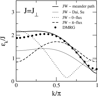
FIG. 16.: Dispersion obtained for a flux-phase approximation of the phase factor with 0-flux (dotted line) and $\pi$-flux (dashed line) through a plaquette. Thick solid line: mean-field dispersion obtained for the meander path in Sec. III A where the correlations related to the phase factor have been taken into account. Thin solid line: dispersion analogous to Dai and Su,[20] where the phase factor has been replaced by its average value. Symbols: one-triplet dispersion obtained by DMRG for a $N$=80-site ladder.[17]

In this appendix we briefly comment on the role of the “phase factor” in the mean-field evaluation of the triplet dispersion. The phase factor $e^{i\pi(n_{\beta_{i}}+n_{\alpha_{i+1}})}$ in Hamiltonian (21) was generated by products of spin operators with site labels not in sequence along the one-dimensional meander path. As the “matrix elements” of the phase operator are $\pm 1$ one might speculate to find a reasonable mean field result by replacing the operator uniformly by $\pm 1$. This corresponds to a flux phase treatment of the phase factor, where the flux through a plaquette is chosen to be 0 and $\pi$, respectively. Applying the same kind of mean field treatment as in Sec. III A one obtains $\epsilon_{k}=|\gamma_{k}|$ for the mean field dispersion, where

$$\gamma_{k}=J_{\perp}(\frac{1}{2}\!-\!\chi_{0})+J\cos k(1\!-\!\chi_{1}\!-\!\chi_{2})+iJ\sin k(\chi_{2}\!-\!\chi_{1})$$

corresponds to zero flux and

$$\gamma_{k}=J_{\perp}(\frac{1}{2}\!-\!\chi_{0})-J\cos k(\chi_{1}\!+\!\chi_{2})+iJ\sin k(1-\chi_{1}\!+\!\chi_{2})$$

to a $\pi$-flux phase. The resulting dispersions are displayed in Fig. 16 together with the mean field dispersion of the meander-path, where (thick solid line) the correlations related to the phase factor are taken into account and where (thin solid line) the phase factor has been replaced by its average value. For comparison also the DMRG results for a $N$=80-site ladder [17] are displayed. Obviously, the form of the dispersion improves considerably when the phase factor is treated in a more adequate way. The simple replacement by a flux phase shows only poor agreement with the DMRG result. It is interesting to note, however, that the spin gap remains finite for all $J_{\perp}/J>0$ within the $\pi$-flux treatment of the phase factor, as has been observed by Azzouz et al. [21] The mean field evaluation of the phase factor (thin solid line) improves the form of the dispersion at least qualitatively. For a reasonable quantitative agreement with the exact dispersion, however, it seems to be necessary to consider also the correlations related to the phase factor (thick solid line).

D Symmetry breaking

A problem of applying the Jordan-Wigner transformation by placing a path throughout the ladder is that both the zigzag and the meander path break symmetries of the original ladder configuration. This problem has already been mentioned in the discussion of the out-of-phase spin-flip correlation function in Sec. III C. The sublattice structure underlying the meander path, see Fig. 5, restricts the translational symmetry along the legs to translations of an even number of sites. Furthermore, it breaks the reflection symmetry with respect to the center line crossing all rungs perpendicularly. In MFA this gives rise to different values for the bond amplitudes $\chi_{1}=\langle\beta_{i}^{\dagger}\alpha_{i+1}\rangle=-0.2679$ and $\chi_{2}=\langle\alpha_{i}^{\dagger}\beta_{i+1}\rangle=0.1777$. Even though the fermionic bond amplitudes have no direct physical meaning, these discrepancies translate into different expectation values for the products of neighboring spin operators. When the spin operators are transformed to fermionic operators according to Eq. (19) and all contractions are replaced by their mean-field values as before, we obtain for the product of the $z$-components $\langle S_{i,\alpha}^{z}S_{i+1,\beta}^{z}\rangle=-|\chi_{2}|^{2}$, $\langle S_{i,\beta}^{z}S_{i+1,\alpha}^{z}\rangle=-|\chi_{1}|^{2}$ and for the $xy$-components $\frac{1}{2}\langle S_{i,\beta}^{+}S_{i+1,\alpha}^{-}+S_{i,\beta}^{-}S_{i+1,\alpha}^{+}\rangle=\chi_{1}$ and $\frac{1}{2}\langle S_{i,\alpha}^{+}S_{i+1,\beta}^{-}+S_{i,\alpha}^{-}S_{i+1,\beta}^{+}\rangle=4\chi_{1}(\chi_{0}^{2}-\chi_{1}\chi_{2})$. Therefore two symmetries are broken with respect to the spin operators: (i) translational symmetry by an odd number of sites as discussed before $\langle S_{i,\alpha}S_{i+1,\beta}\rangle\neq\langle S_{i+1,\beta}S_{i+2,\alpha}\rangle$ and (ii) rotational symmetry in spin space $\langle S_{i,\alpha}^{z}S_{i+1,\beta}^{z}\rangle\neq\frac{1}{4}\langle S_{i,\alpha}^{+}S_{i+1,\beta}^{-}+S_{i,\alpha}^{-}S_{i+1,\beta}^{+}\rangle$.

The physical interpretation of breaking the translational symmetry is quite obvious. $\langle S_{i,\alpha}S_{i+1,\beta}\rangle\neq\langle S_{i+1,\beta}S_{i+2,\alpha}\rangle$ signifies that a static dimerization pattern is induced along the meander path. Its amplitude, however, is very small $\langle S_{i+1,\beta}S_{i+2,\alpha}-S_{i,\alpha}S_{i+1,\beta}\rangle=0.037$. A staggered dimerization pattern of this kind can, e.g., be induced by consideration of a 4-spin cyclic exchange interaction [40] of about $J_{cyc}/J\approx 1-2$. Indeed, it has been found that the inclusion of a cyclic spin exchange is necessary in order to obtain a consistent description of the experimental data for cuprate spin ladder compounds like (La,Ca)₁₄Cu₂₄O₄₁. [17] The realistic value of $J_{cyc}\approx 0.2-0.27J_{\perp}$, however, is not strong enough to induce a static dimerization pattern. Nevertheless the correlation length for dimerization fluctuations increases with cyclic spin exchange and the dip in the one–triplet dispersion is reduced. [17] This could to some extent explain the good agreement we find for our Jordan-Wigner calculation with the experimental spectra of (La,Ca)₁₄Cu₂₄O₄₁, as our artificial symmetry breaking seems to imitate some of the effects of a cyclic spin exchange.

REFERENCES

• [1] E. Dagotto and T.M. Rice, Science 271, 618 (1996).
• [2] T.M. Rice, S. Gopalan, and M. Sigrist, Europhys. Lett. 23,445 (1993).
• [3] M. Azuma, Z. Hiroi, M. Takano, K. Ishida, and Y. Kitaoka, Phys. Rev. Lett. 73, 3463 (1994).
• [4] S. Chakravarty, B.I. Halperin, and D.R. Nelson, Phys. Rev. Lett. 60, 1057 (1988); Phys. Rev. B 39, 2344 (1989).
• [5] D.V. Khveshchenko, Phys. Rev. B 50, 380 (1994).
• [6] G. Sierra, J. Phys. A 29, 3299 (1996); cond-mat/9610057.
• [7] S. Chakravarty, Phys. Rev. Lett. 77, 4446 (1996).
• [8] S. Chakravarty, B.I. Halperin, and D.R. Nelson, Phys. Rev. B 39, 2344 (1989).
• [9] S. Sachdev and R. N. Bhatt, Phys. Rev. B 41, 9323 (1990).
• [10] S. Gopalan, T. M. Rice and M. Sigrist, Phys. Rev. B 49, 8901 (1994).
• [11] O.P. Sushkov and V.N. Kotov, Phys. Rev. Lett. 81, 1941 (1998); V.N. Kotov, O.P. Sushkov, and R. Eder, Phys. Rev. B 59, 6266 (1999).
• [12] S. Trebst, H. Monien, C.J. Hamer, Z. Weihong, and R.R.P. Singh, Phys. Rev. Lett. 85, 4373 (2000); W. Zheng, C.J. Hamer, R.R.P. Singh, S. Trebst, and H. Monien, Phys. Rev. B 63, 144410 (2001).
• [13] D. G. Shelton, A. A. Nersesyan and A. M. Tsvelik, Phys. Rev. B 53, 8521 (1996).
• [14] M. Greiter, Phys. Rev. B 65, 134443 (2002); Phys. Rev. B 66, 054505 (2002).
• [15] D. C. Johnston, M. Troyer, S. Miyahara, D. Lidsky, K. Ueda, M. Azuma, Z. Hiroi, M. Takano, M. Isobe, Y. Ueda, M. A. Korotin, V. I. Anisimov, A. V. Mahajan, and L. L. Miller, cond-mat/0001147.
• [16] M. Windt, M. Grüninger, T. Nunner, C. Knetter, K. P. Schmidt, G. S. Uhrig, T. Kopp, A. Freimuth, U. Ammerahl, B. Büchner, and A. Revcolevschi, Phys. Rev. Lett. 87, 127002 (2001).
• [17] T. S. Nunner, P. Brune, T. Kopp, M. Windt, and M. Grüninger, cond-mat/0203472.
• [18] P. Jordan and E. Wigner, Z. Phys. 47, 631 (1928).
• [19] More recent discussions of the exploitation of the Jordan-Wigner transformation, in the context of field theories for strongly correlated electron systems, can be found in the following two textbooks: A.M. Tsvelik, Quantum Field Theory in Condensed Matter Physics, (Cambridge University Press, 1995); E. Fradkin, Field Theories of Condensed Matter Systems, (Addison-Wesley, 1991).
• [20] X. Dai, and Z. Su, Phys. Rev. B 57, 964 (1998).
• [21] M. Azzouz, L. Chen, and S. Moukouri, Phys. Rev. B 50, 6233 (1994).
• [22] J. Lorenzana and G. A. Sawatzky, Phys. Rev. Lett. 74, 1867 (1995); Phys. Rev. B 52, 9576 (1995).
• [23] C. Knetter, K. P. Schmidt, M. Grüninger, and G. S. Uhrig, Phys. Rev. Lett 87, 167204 (2001).
• [24] H. Suzuura, H. Yasuhara, A. Furusaki, N. Nagaosa, and Y. Tokura, Phys. Rev. Lett. 76, 2579 (1996).
• [25] Y. R. Wang, Phys. Rev. B 46, 151 (1992).
• [26] T. Yamada, Prog. Theor. Phys. Jpn. 41, 880 (1969).
• [27] J. Lorenzana and R. Eder, Phys. Rev B 55, R3358 (1997).
• [28] G. Müller, H. Thomas, H. Beck, and J.C. Bonner, Phys. Rev. B 24, 1429 (1981).
• [29] A.H. Bourgourzi, M. Couture, and M. Kacir, Phys. Rev. B 54, R12669 (1996).
• [30] M. Karbach, G. Müller, A.H. Bougourzi, A. Fledderjohann, and K.-H. Müetter, Phys. Rev. B 55, 12510 (1997).
• [31] Jordan Wigner transformation in two dimensions: E. Fradkin, Phys. Rev. Lett. 63, 322 (1989); D. Eliezer and G.W. Semenoff, Phys. Lett. B 286, 118 (1992); the treatment of two dimensional systems has recently been reviewed by O. Derzhko, Journal of Physical Studies v. 5, No. 1, 49 (2001).
• [32] Jordan Wigner transformation in three dimensions: L. Huerta and J. Zanelli, Phys. Rev. Lett. 71, 3622 (1993).
• [33] K. Damle and S. Sachdev, Phys. Rev. B 57, 8307 (1998).
• [34] G.S. Uhrig and H.J. Schulz, Phys. Rev. B 54, R9624 (1996); erratum ibid. 58, 2900 (1998)
• [35] C. Jurecka and W. Brenig, Phys. Rev. B 61, 14307 (2000).
• [36] M. Grüninger, M. Windt, T. Nunner, C. Knetter, K. P. Schmidt, G.S. Uhrig, T. Kopp, A. Freimuth, U. Ammerahl, B. Büchner, A. Revcolevschi, cond-mat/0109524.
• [37] P. J. Freitas and R. R. P. Singh, Phys. Rev. B 62, 14113 (2000).
• [38] K. P. Schmidt, C. Knetter, and G. S. Uhrig, Europhys. Lett. 56, 877 (2001).
• [39] T. S. Nunner, P. Brune and T. Kopp, to be published.
• [40] A. Läuchli, G. Schmid, and M. Troyer, cond-mat/0206153.