Dynamical model of financial markets: fluctuating ‘temperature’ causes intermittent behavior of price changes

Abstract

We present a model of financial markets originally proposed for a turbulent flow, as a dynamic basis of its intermittent behavior. Time evolution of the price change is assumed to be described by Brownian motion in a power-law potential, where the ‘temperature’ fluctuates slowly. The model generally yields a fat-tailed distribution of the price change. Specifically a Tsallis distribution is obtained if the inverse temperature is $\chi^{2}$-distributed, which qualitatively agrees with intraday data of foreign exchange market. The so-called ‘volatility’, a quantity indicating the risk or activity in financial markets, corresponds to the temperature of markets and its fluctuation leads to intermittency.

,

1 Introduction

Financial returns are known to be non-gaussian and exhibit fat-tailed distribution fa65 -hkk01 . The fat tail relates to intermittency — an unexpected high probability of large price changes, which is of utmost importance for risk analysis. The recent development of high-frequency data bases makes it possible to study the intermittent market dynamics on time scales of less than a day ms00 -hkk01 .

Using foreign exchange (FX) intraday data, Müller et al. mdd97 showed that there is a net flow of information from long to short timescales, i.e., the behavior of long-term traders influences the behavior of short-term traders. Motivated by this hierarchical structure, Ghashghaie et al. gbp96 have discussed analogies between the market dynamics and hydrodynamic turbulence fr95 ; cgh90 , and claimed that the information cascade in time hierarchy exists in a FX market, which corresponds to the energy cascade in space hierarchy in a three-dimensional turbulent flow. These studies have stimulated further investigations on similarities and differences in statistical properties of the fluctuations in the economic data and turbulence ms96 -bgt00 . Differences have also emerged. Mantegra and Stanley ms96 ; ms97 and Arneodo et al. abc96 pointed out that the time evolution, or equivalently the power spectrum is different for the price difference (nearly white spectrum) and the velocity difference ($f^{1/3}$ spectrum, i.e., $-5/3$-law for the spectrum of the velocity). Moreover, from a parallel analysis of the price change data with time delay and the velocity difference data with time delay (equivalent to the velocity difference data with spatial separation under the Taylor hypothesis fr95 ), it was shown that the time evolution of the second moment and the shape of the probability density function (PDF), i.e., the deviation from gaussian PDF are different in these two stochastic processes ms97 . On the other hand, non-gaussian character in fully developed turbulence fr95 has been linked with the nonextensive statistical physics ts88 -bls01 .

As dynamical foundation of nonextensive statistics, Beck recently proposed a new model describing hydrodynamic turbulence be01 ; be01a . The velocity difference $\Delta v$ of two points in a turbulent flow with the spatial separation $\Delta r$ is described by Brownian motion (an overdamped Langevin equation ri89 ) in a power-law potential. Assuming a $\chi^{2}$-distribution for the inverse temperature, he obtained a Tsallis distribution ts88 for $\Delta v$. However, if we take into account the almost uncorrelated behavior of the price change ms96 -ms97 , the picture by means of the Brownian motion seems to be more appropriate for the market data rather than turbulence. Moreover, the description by the Langevin equation is able to relate the PDF of the price change to that of the volatility, a quantity known as a measure of the risk in the market. Thus we applied the model to FX market dynamics by employing the correspondence by Ghashghaie et al. gbp96 .

2 Model

We substitute the FX price difference $Z(t)\equiv y(t+\Delta t)-y(t)$ with the time delay $\Delta t$ for the velocity difference $\Delta v$ with the spatial separation $\Delta r$. Beck’s model for turbulence then reads

$$\frac{dZ}{dt}=\gamma F(Z)+R(t),$$ (1)

where $\gamma>0$ is a constant, and $R(t)$ is gaussian white noise corresponding to the temperature $kT$, satisfying $\left<R(t)R(t^{\prime})\right>=2\gamma kT\delta(t-t^{\prime})$. The ‘force’ $F=-\partial U(Z)/\partial Z$ is assumed to be obtained by a power-law potential $U(Z)=C|Z|^{2\alpha}$ with an exponent $2\alpha$, where $0<\alpha\leq 1$ and $C$ is a positive constant. That is, the system is subject to a restoring force proportional to the power of the price difference, $|Z|^{2\alpha}$ besides the random force $R(t)$. Especially when $\alpha=1$, the restoring force is linear to $Z$. Under a constant temperature $kT$, Eq. (1) leads to a stationary (i.e., thermal equilibrium) distribution of $Z$ as

$$P_{\Delta t}(Z|\beta)=\frac{e^{-\beta U(Z)}}{\int e^{-\beta U(Z)}dZ}=\frac{\alpha}{\Gamma(\frac{1}{2\alpha})}(C\beta)^{1/2\alpha}e^{-\beta C|Z|^{2\alpha}},$$ (2)

where $\beta\equiv 1/kT$ is the inverse temperature be01 . The ‘local’ variance of $Z$, which is defined for a fixed value of $\beta$, is obtained from the conditional probability in Eq. (2) as

$$\left<Z^{2}\right>_{\beta}=\int Z^{2}P_{\Delta t}(Z|\beta)dZ=\frac{\Gamma(\frac{3}{2\alpha})}{\Gamma(\frac{1}{2\alpha})}(C\beta)^{-1/\alpha}\propto{(kT)}^{1/\alpha}.$$ (3)

We define the volatility by the square root of the local variance of $Z$ (see Eq. (9)). When $\alpha=1$ and $C=1/2$, $\left<Z^{2}\right>_{\beta}$ coincides with the temperature and the conditional PDF reduces to gaussian, while for $\alpha\neq 1$, $\{\left<Z^{2}\right>_{\beta}\}^{\alpha}$ is proportional to $kT$.

Let us assume that the ‘temperature’ of the FX market is not constant and fluctuates in larger time scales, and $\beta$ is, just as in Beck’s model for turbulence, $\chi^{2}$-distributed with degree $n$:

$$f_{\Delta t}(\beta)\equiv\frac{1}{\Gamma(\frac{n}{2})}\left(\frac{n}{2\beta_{0}}\right)^{n/2}\beta^{n/2-1}\exp\left(-\frac{n\beta}{2\beta_{0}}\right),\qquad n>2\,,$$ (4)

where $\Gamma$ is the Gamma function, $\beta_{0}$ is the average of the fluctuating $\beta$ and $n$ relates to the relative variance of $\beta$:

$$\left<\beta\right>=\beta_{0},\qquad\frac{\left<\beta^{2}\right>-\left<\beta\right>^{2}}{\left<\beta\right>^{2}}=\frac{2}{n}\,.$$ (5)

Equation (4) implies that the local variance $\left<Z^{2}\right>_{\beta}\equiv v$ fluctuates with the distribution $p(v)\propto v^{-(\alpha+1)}f_{\Delta t}(v^{-\alpha})$. The conditional probability in Eq. (2) together with Eq. (4) yields a Tsallis-type distribution ts88 ; be01 for the ultimate PDF of $Z$:

$$P_{\Delta t}(Z) = \int P_{\Delta t}(Z|\beta)f_{\Delta t}(\beta)d\beta=\frac{1}{Z_{q}}\frac{1}{\left\{1+\frac{C\beta_{0}2\alpha(q-1)|Z|^{2\alpha}}{2\alpha-(q-1)}\right\}^{1/(q-1)}}\;,$$ (6)

$$\frac{1}{Z_{q}} = \alpha\left\{\frac{C\beta_{0}2\alpha(q-1)}{2\alpha-(q-1)}\right\}^{1/2\alpha}\frac{\Gamma\left(\frac{1}{q-1}\right)}{\Gamma(\frac{1}{2\alpha})\Gamma(\frac{1}{q-1}-\frac{1}{2\alpha})}\,,$$ (7)

where Tsallis’ nonextensivity parameter $q$ is defined by

$$q\equiv 1+\frac{2\alpha}{\alpha n+1}\,,$$ (8)

which satisfies $1<q<5/3$ because of $0<\alpha\leq 1$ and $n>2$. Since $q>1$, the distribution of $Z$ exhibits power-law tails for large $Z$: $P_{\Delta t}(Z)\sim Z^{-2\alpha/(q-1)}=Z^{-(\alpha n+1)}$. Hence, the $m$th moment $\left<Z^{m}\right>=\int Z^{m}P_{\Delta t}(Z)dZ$ converges only for $m<\alpha n$. In the limit of $q\rightarrow 1$, $P_{\Delta t}(Z)$ in Eq. (6) reduces to the canonical distribution of extensive statistical mechanics: $\lim_{q\rightarrow 1}P_{\Delta t}(Z)=P_{\Delta t}(Z|\beta_{0})$.

3 Results and discussions

We have applied the present model to the same FX market data set as used in Ref. gbp96 (provided by Olsen and Associates oa93 which consists of 1 472 241 bid-ask quotes for US dollar-German mark exchange rates during the period October 92 - September 93). The volatility is often estimated by the standard deviation of the price change in an appropriate time window ms00 . Employing this definition, we express the volatility in terms of the local standard deviation of the price change $Z(t_{i})\equiv y(t_{i}+\Delta t)-y(t_{i})$ as

$$V\equiv\sqrt{\frac{1}{N}\sum_{j=1}^{N}\left\{Z(t_{j})\right\}^{2}}\,.$$ (9)

Here the window size has been chosen as $N=35$. Since $V^{-2\alpha}$ corresponds to $\beta$ (see Eq. (3)) which is $\chi^{2}$-distributed, $n$ can be explicitly obtained from the relative variance of $\beta$ using Eq. (5). Thus, there is only one adjustable parameter among $(\alpha,q,n)$, because we have another relation, Eq. (8). In other words, the PDF, $P_{\Delta t}(Z)$ of the price change and the PDF, $f_{\Delta t}(\beta)$ of the inverse power $V^{-2\alpha}\equiv\beta$ of the volatility are determined simultaneously once the value of $\alpha$ has been specified.

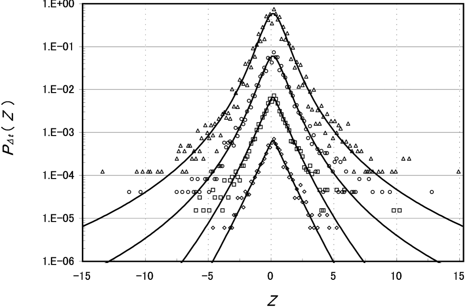
Figure 1: Data points: standardized PDF $P_{\Delta t}(Z)$ of price changes $Z(t)\equiv y(t+\Delta t)-y(t)$ for time delays $\Delta t=$ 320 s, 1 280 s, 5 120 s, 20 480 s (from top to bottom). The middle prices $y(t)\equiv(y_{\rm bid}(t)+y_{\rm ask}(t))/2$ have been used (data provided by Olsen and Associates oa93 ). The PDF has been obtained in a similar way as Ref. ms95 , i.e., we have selected the complete set of non-overlapping records separated by a time interval $\Delta t(1\pm\epsilon)$ with the tolerance $0<\epsilon<0.035$. The number of the available data points thus decreases with $\Delta t$, which is 54 087, 16 338, 4 359, 1 114 (from top to bottom). For better visibly, the curves have been vertically shifted with respect to each other. Full lines: theoretical expression given in Eq. (6) in text, where $(\alpha,q,n)$ is (0.918, 1.393, 4), (0.832, 1.322, 5), (0.565, 1.101, 18), (0.540, 1.054, 35) (from top to bottom). $n$ is explicitly decided from the variance of the volatility data (the closest integer satisfying Eq. (5)), $q$ is from Eq. (8), so that we only need to adjust $\alpha$ by least square fitting.

The PDF’s with time delay $\Delta t$ varying from five minutes up to approximately six hours are displayed in Fig.1 together with theoretical curves obtained from Eq. (6). As the time scale $\Delta t$ increases, $n$ increases, while $\alpha$ and $q$ decrease. The nonextensivity parameter $q$ tends to the extensive limit: $q\rightarrow 1$ as $\Delta t$ increases. Using the same parameter values $(\alpha,q,n)$, the PDF’s of $\beta$ are compared in Fig. 2.

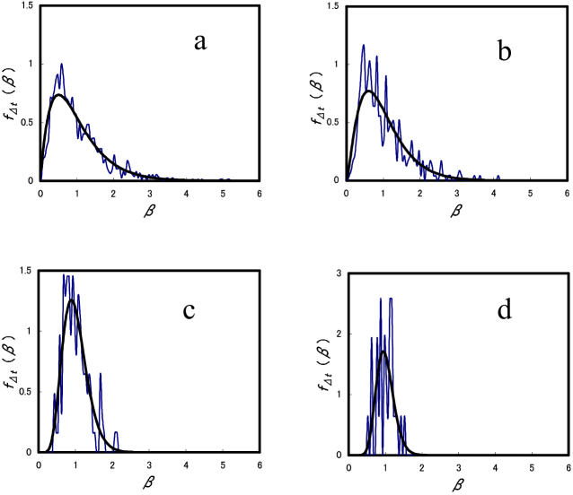
Figure 2: Rescaled probability density $f_{\Delta t}(\beta)$ of the quantity $V^{-2\alpha}\equiv\beta$, where $V$ is the volatility defined by the local standard deviation of the price change $Z(t)$. (See the legend of Fig. 1 for the definition of $Z(t)$.) Thin lines: obtained from the volatility data, which was defined by $V(t_{i})\equiv\sqrt{\sum_{j=1}^{N}\left\{Z(t_{N(i-1)+j})\right\}^{2}/N}$ with $N=35$ so that the windows for different volatility data points do not overlap. The number of the available data points is 1 545, 466, 124, 24 (from a to d). The data set has been rescaled so that the average of $\beta$ is unity: $\left<\beta\right>=\left<V^{-2\alpha}\right>=1$. Thick lines: $\chi^{2}$-distribution for $\beta$ given in Eq. (4) with $\beta_{0}=1$. The same parameter values as in Fig. 1 are used, where $n$ is the integer closest to $2/\left(\left<\beta^{2}\right>-1\right)$ (see Eq. (5) in text), $\alpha$ has been adjusted by least square fitting of $P_{\Delta t}(Z)$ in Fig. 1. ($\alpha,q,n$) is (0.918, 1.393, 4), (0.832, 1.322, 5), (0.565, 1.101, 18), (0.540, 1.054, 35) (from a to d).

The average ‘temperature’ in the market $1/\beta_{0}\sim\left<Z^{2}\right>^{\alpha}\sim(\Delta t)^{\alpha\zeta_{2}}$ increases with $\Delta t$ since $\alpha\zeta_{2}$ is positive. (We obtained the scaling exponent gbp96 ; fr95 $\zeta\approx 0.85$, which is larger than 2/3 obtained for turbulence.) In contrast, the fluctuation of the temperature increases with decreasing $\Delta t$ because the variance of the inverse temperature is proportional to $2/n$. The smaller values of $n$ imply the stronger intermittency which occurs in small time scales. The intermittent character in the price change can be seen as a fat tail of $P_{\Delta t}(Z)$ in Fig. 1. Also in Fig. 2, the peak of $f_{\Delta t}(\beta)$ shifts to smaller $\beta$ as $\Delta t$ decreases (from d to a in Fig. 2), which means relatively high temperatures are realized more frequently in short time scales.

It should be noted that the PDF in Eq. (6) with $\alpha=1$ reduces to Student’s $t$-distribution ms00 , which has often been used to characterize the fat tails hkk01 . When $\alpha=1$, there is no adjustable parameter because $n$ is decided from Eq. (5). The FX market system is then subject to a restoring force linear to the price change and the volatility is proportional to the temperature. We have found that the PDFs of $Z$ and $\beta$ reproduce, although very roughly, the Olsen and Associates’ data points even if $\alpha$ is fixed at $\alpha=1$. However, adjusting the parameter $\alpha$ improved the line shape of $P_{\Delta t}(Z)$ in a range close to $Z=0$. The data points in Fig. 1 exhibit a cusp at $Z=0$ for large time scales $\Delta t$, which implies a singularity of the second derivative of the PDF at $Z=0$. The larger reduction of $\alpha$ from unity leads to the stronger singularity. (Note that the factor $|Z|^{2\alpha-2}$ arises from $d^{2}P_{\Delta t}(Z)/dZ^{2}$.) Thus the better fitting for large $\Delta t$ was obtained from a reduced value of $\alpha$. The trend of decrease in $\alpha$ with increasing $\Delta t$ was observed for the turbulent flow be01 as well. However, the deviation from $\alpha=1$ is much smaller than the present case and the cusp is invisible.

Ghashghaie et al. gbp96 have used a model for turbulence by Castaing et al. cgh90 , in which a log-normal distribution has been assumed for the local standard deviation of the price change. The present model reduces to the model by Ghashghaie et al. if the stochastic process given in Eq. (1) is assumed with $\alpha=1$ (the local variance of $Z$ is then proportional to $kT$) and the $\chi^{2}$-distribution for $\beta$ (the inverse of the local variance of $Z$) is replaced by the log-normal distribution for $\sqrt{kT}$ (the local standard deviation of $Z$). Although no analytic expression like Eq. (6) for $P_{\Delta t}(Z)$ is obtained, a similar qualitative explanation can be applied to their model: The volatility (or equivalently, the square root of the temperature) fluctuates slowly with a log-normal distribution, and the smaller time scale corresponds to the larger variance of the logarithm of the volatility. (The variance is denoted by $\lambda^{2}$ in Ref. 4.) However, the power-law behavior of the tail of the volatility distribution lgc99 can be better described by the $\chi^{2}$-distribution for the inverse of the variance.

We have proposed the stochastic process described by Eq. (1) for FX market dynamics in small time scales. In fact, Eq. (1) is the simplest stochastic process which can realize the thermal equilibrium distribution, Eq. (2) in the power-law potential. More realistic and more complicated processes that assure convergence to Eq. (2) at local temperatures might be possible. Mantegna and Stanley have proposed a different stochastic model of the price change, which is described by a truncated Levy flight (TLF) ms95 ; ms00 . The model, yielding approximately a stable distribution, well reproduces the self-similar property of PDF at different time scales: $\Delta t=$ 1 min to 1 000 min. However, the parameters $\alpha$ and $\gamma$ characterizing the stable distribution fluctuate for larger (monthly) time scales ms00 , where $\gamma$ gives a measure of the volatility. In other words, the ultimate distribution (let us denote it $P^{\rm TLF}_{\Delta t}(Z)$) should be obtained, like Eq. (6), from the weighted average over these parameters. A difference between $P^{\rm TLF}_{\Delta t}(Z)$ and $P_{\Delta t}(Z)$ is that $P^{\rm TLF}_{\Delta t}(Z)$ has no cusp at $Z=0$: $P^{\rm TLF}_{\Delta t}(Z)\sim 1-AZ^{2}$ for $|Z|\ll 1$, whereas $P_{\Delta t}(Z)\sim 1-A|Z|^{2\alpha}$, and the present FX date set indeed exhibits a cusp as seen in Fig. 1.

Finally, a fundamental question has been left open: How to derive theoretically the increasing trend of fat-tailed character with decreasing time scale, i.e., $\Delta t$-dependence of the parameters ($\alpha,q,n$). An attempt to derive the non-gaussian fat-tailed character in small time scales was made by Friedlich et al. recently fpr00 . They derived a multiplicative Langevin equation from a Fokker-Planck equation and showed that the equation becomes more multiplicative and hence fat-tailed as $\Delta t$ decreases. Clarifying the relation between their multiplicative Langevin equation and Eq. (1) (the latter being rather simple although including the fluctuating temperature) should be important as well as interesting.

Acknowledgments

We would like to thank Professor T. Watanabe for valuable comments. The FX data set was provided by Olsen and Associates.

References

- (1) E. F. Fama, J. Business 38 (1965) 34.
- (2) R. N. Mantegna, H. E. Stanley, An Introduction to Econophysics: Correlations and Complexity in Finance, Cambridge Univ. Press, Cambridge, 2000.
- (3) L. Bauwens, P. Giot, Econometric Modelling of Stock Market Intraday Activity, Kluwer Acad. Publishers, Boston, 2001.
- (4) S. Ghashghaie, W. Breymann, J. Peinke, P. Talkner, Y. Dodge, Nature 381 (1996) 767.
- (5) R. N. Mantegna, H. E. Stanley, Nature 383 (1996) 587.
- (6) A. Arneodo, J. -P. Bouchaud, R. Cont, J. -F. Muzy, M. Potters, D. Sornette, Cond-mat /9607120.
- (7) R. N. Mantegna, H. E. Stanley, Physica A 239 (1997) 255.
- (8) A. Arneodo, J. -F. Muzy, D. Sornette, Eur. Phys. J. B2 (1998) 277.
- (9) R. Friedrich, J. Peinke, Ch. Renner, Phys. Rev. Lett. 84 (2000) 5224.
- (10) W. Breymann, S. Ghashghaie, P. Talkner, Int. J. Theor. Appl. Finance 3 (2000) 357.
- (11) C. A. E. Goodhart, M. O’Hara, J. Emp. Finance 4 (1997) 73.
- (12) U. A. Müller, M. M., Dacorogna, R. D. Davé, R. B. Olsen, O. V. Pictet, J. E. von Weizsäcker, J. Emp. Finance 4 (1997) 213.
- (13) R. N. Mantegna, H. E. Stanley, Nature 376 (1995) 46.
- (14) Y. Liu, P. Gopikrishnan, P. Cizeau, M. Meyer, C. -K. Peng, H. E. Stanley, Phys. Rev. E 60 (1999) 1390.
- (15) R. Huisman, K. G. Koedijk, C. J. M. Kool, F. Palm, J. Business and Economic Statistics 19 (2001) 208.
- (16) U. Frisch, Turbulence: the Legacy of A. N. Kolmogorov, Cambridge Univ. Press, Cambridge, 1995.
- (17) B. Castaing, Y. Gagne, E. J. Hopfinger, Physica D 46 (1990) 177.
- (18) C. Tsallis, J. Stat. Phys. 52 (1988) 479.
- (19) G. Wilk, Z. Włodarczyk, Phys. Rev. Lett. 84 (2000) 2770.
- (20) T. Arimitsu, N. Arimitsu, Prog. Theor. Phys. 105 (2001) 355.
- (21) C. Beck, Phys. Rev. Lett. 87 (2001) 180601.
- (22) C. Beck, Physica A 295 (2001) 195.
- (23) C. Beck, G. S. Lewis, H. L. Swinney, Phys. Rev. 63 E (2001) 035303.
- (24) H. Risken, The Fokker-Planck Equation: Methods of Solution and Applications, 2nd edn, Springer-Verlag, Berlin, 1989.
- (25) High Frequency Data in Finance 1993, Olsen and Associates, Zurich.