ORIGIN OF THE VIOLATION OF THE FLUCTUATION-DISSIPATION THEOREM IN SYSTEMS WITH ACTIVATED DYNAMICS

Abstract

We analyze the validity of the fluctuation-dissipation theorem for slow relaxation systems in the context of mesoscopic nonequilibrium thermodynamics. We demonstrate that the violation arises as a natural consequence of the elimination of fast variables in the description of a glassy system, and it is intrinsically related to the underlying activated nature of slow relaxation. In addition, we show that the concept of effective temperature, introduced to characterize the magnitude of the violation, is not robust since it is observable-dependent, can diverge, or even be negative.

Many nonequilibrium systems in nature evolve in time following slow relaxation processes. Examples of this behavior are usually encountered in glassy systems sitges , polymers angell2 , granular flows nagel , foams cates , and crumpled materials nagel2 to mention just a few. A complete and satisfactory characterization of these systems constitutes nowadays one of the most challenging issues of nonequilibrium statistical physics. The main feature of slow processes is that the relaxation time may exceed significantly the observation time scale in such a way that the system can be considered as being permanently out of equilibrium. This peculiarity is the origin of a distinctive behavior which differs markedly from the case in which relaxation occurs in shorter time scales. The existence of aging regimes kurchan and the violation of the fluctuation-dissipation theorem (FDT) cugliand-pre constitute examples of this behavior.

For all these reasons, the straightforward application of equilibrium concepts, appropriate to describe fast relaxation processes, to out of equilibrium situations, inherent to slow relaxation dynamics, becomes in principle doubtful. However, our purpose in this Letter is to show that, when nonequilibrium thermodynamic concepts are applied at the mesoscopic level jm , one may justify many of the peculiarities of the behavior observed in glassy systems. In particular, we will show that the violation of FDT is a natural consequence of the activated nature of the dynamics of a slow relaxing system. Starting from a more detailed description in which the system can be safely considered as near equilibrium and evolves via a diffusion process, we will show that the implicit elimination of the fast variables, leads to an activated regime where the system becomes far from equilibrium and consequently the FDT is not fulfilled. Coarsening the level of description is then the origin of the violation of the FDT in strong glasses. Precisely, one way to characterize this violation is through the concept of effective temperature. We will also discuss the validity and robustness of this concept.

It is well established that the evolution of many systems can be described in terms of its energy landscape angell ; debene-stilinger , representing the (free) energy as a function of an order parameter or reaction coordinate $\gamma$ oppenheim . Complex systems exhibit a very intricate landscape with a great multiplicity of wells separated by barriers. Whereas at high temperatures the system may explore the whole landscape at low enough temperatures the dynamics reduces basically to two elementary processes: a fast relaxation toward the local minima via a diffusion process, and a slow activated process in which the system overcomes the barrier toward the next minimum. The presence of the barriers is thus the cause for the slow evolution of the system. Hence, the case of a single barrier captures the essential mechanism of the slow dynamics. To show how the activated nature of the slow evolution of the system can be responsible of some of the peculiarities of the response of glasses we will then focus on the simplified model of a bistable potential.

It is then plausible to assume that the evolution of the system occurs via a diffusion process through its potential landscape parameterized by the $\gamma$-coordinate, which will be characterized by the diffusion current $J(\gamma,t)$ and the corresponding chemical potential $\mu(\gamma,t)$. As any diffusion process, it can be treated in the framework of nonequilibrium thermodynamics degroot . Assuming local equilibrium in $\gamma$-space, variations of the entropy $\delta s$ related to changes in the probability density $\rho(\gamma,t)$ are given through the Gibbs equation

$$\delta s=-\frac{1}{T}\int\mu\left(\gamma,t\right)\delta\rho\left(\gamma,t\right)d\gamma,$$ (1)

where $T$ is the temperature.

The entropy production inherent to the diffusion process, $\sigma\equiv\partial s/\partial t$,

$$\sigma=-\frac{1}{T}\int J(\gamma,t)\frac{\partial}{\partial\gamma}\mu(\gamma,t)d\gamma,$$ (2)

follows from Eq. (1), after using the continuity equation in $\gamma$-space,

$$\frac{\partial}{\partial t}\rho\left(\gamma,t\right)=-\frac{\partial}{\partial\gamma}J\left(\gamma,t\right).$$ (3)

From that expression one then infers the relation between current and thermodynamic “force” $J\left(\gamma,t\right)=-\frac{1}{T}\int L(\gamma,\gamma^{\prime})\frac{\partial}{\partial\gamma^{\prime}}\mu(\gamma^{\prime},t)d\gamma^{\prime}.$ The assumptions of locality in $\gamma$-space, for which $L(\gamma,\gamma^{\prime})=L(\gamma)\delta(\gamma-\gamma^{\prime})$, and ideality, imposing the form of the chemical potential $\mu\left(\gamma,t\right)=k_{B}T\ln\rho\left(\gamma,t\right)+\Phi\left(\gamma\right)$, with $k_{B}$ being the Boltzmann constant, and $\Phi\left(\gamma\right)$ the bistable potential, provide the diffusion current in $\gamma$-space

$$J\left(\gamma,t\right)=-De^{-\Phi/k_{B}T}\frac{\partial}{\partial\gamma}e^{\mu/k_{B}T},$$ (4)

where $D=k_{B}L/\rho$ is the diffusion coefficient, taken to be constant as a first approximation. When this phenomenological relation is substituted into the continuity equation (3) one obtains the diffusion equation

$$\frac{\partial}{\partial t}\rho\left(\gamma,t\right)=\frac{\partial}{\partial\gamma}D\left(\frac{\partial}{\partial\gamma}\rho\left(\gamma,t\right)+\frac{\rho(\gamma,t)}{k_{B}T}\frac{\partial}{\partial\gamma}\Phi(\gamma)\right),$$ (5)

which governs the evolution of the average probability density. This result agrees with the one derived from a master equation oppenheim , and indicates that nonequilibrium thermodynamics can be used at mesoscopic level to provide the fundamental kinetic laws of the Fokker-Planck type governing the dynamics.

The probability density is subjected to fluctuations, which may be introduced through a random contribution to the current, $J^{r}\left(\gamma,t\right)$, in Eq. (3) ignacio , satisfying the fluctuation-dissipation theorem in $\gamma$-space

$$\left\langle J^{r}\left(\gamma,t\right)J^{r}\left(\gamma^{\prime},t^{\prime}\right)\right\rangle=2D\left\langle\rho\left(\gamma,t\right)\right\rangle\delta(\gamma-\gamma^{\prime})\delta(t-t^{\prime}),$$ (6)

where $\left\langle\rho\left(\gamma,t\right)\right\rangle$ is the solution of Eq. (5). The formulation of a FDT is intimately related to the fact that the system is in local equilibrium in $\gamma$-space.

When the height of the energy barrier separating the two minima of the potential is large compared to thermal energy, which happens at low enough temperatures, a fast relaxation toward the local minima occurs, and the system achieves a state of quasi-equilibrium characterized by equilibration in each well. The chemical potential then becomes a piece-wise continuous function of the coordinates, $\mu\left(\gamma,t\right)=\mu\left(\gamma_{1},t\right)\Theta\left(\gamma_{o}-\gamma\right)+\mu\left(\gamma_{2},t\right)\Theta\left(\gamma-\gamma_{o}\right),$ and consequently the probability density achieves the form

$$\rho\left(\gamma,t\right) = \rho_{1}\left(t\right)e^{-\left\{\Phi\left(\gamma\right)-\Phi\left(\gamma_{1}\right)\right\}/k_{B}T}\Theta\left(\gamma_{o}-\gamma\right)$$ (7)

$$\>+ \rho_{2}\left(t\right)e^{-\left\{\Phi\left(\gamma\right)-\Phi\left(\gamma_{2}\right)\right\}/k_{B}T}\Theta\left(\gamma-\gamma_{o}\right).$$

Here $\rho_{1}\left(t\right)\equiv\rho(\gamma_{1},t)$ and $\rho_{2}\left(t\right)\equiv\rho(\gamma_{2},t)$ are the values of the probability density at the minima, $\Theta\left(x\right)$ is the unit step function, and $\gamma_{o}$, $\gamma_{1}$, and $\gamma_{2}$ are the coordinates of the maximum, and the minima of the potential, respectively.

Hence, once the fast relaxation toward the local minima has occurred, the evolution of the system proceeds by jumps from one well to the other undergoing an activated process. In this situation, a contracted description performed in terms of the populations at the wells can be adopted. This description corresponds to that of the two level model for a glass fisher ; langer , a minimal model which evolves according to an activated dynamics hanggi conferring him the characteristic aging properties of glasses, closely related to hysteresis langer2 . Defining the integrated probability $N(\gamma,t)=\int^{\gamma}_{-\infty}d\gamma^{\prime}\rho(\gamma^{\prime},t),$ and by integration of the continuity equation (3) we obtain

$$\frac{\partial}{\partial t}N\left(\gamma,t\right)=-J^{s}\left(\gamma,t\right)-J^{r}\left(\gamma,t\right).$$ (8)

To proceed with the contraction of the dynamics from the diffusion regime to the two level regime we will introduce the integral operator $P$ acting on a function in $\gamma$-space as

$$P\psi(\gamma)=\frac{1}{\int^{\gamma_{2}}_{\gamma_{1}}\,d\gamma e^{\Phi/k_{B}T}}\int^{\gamma_{2}}_{\gamma_{1}}\,d\gamma e^{\Phi/k_{B}T}\psi(\gamma).$$ (9)

Projecting both sides of Eq. (8) with $P$, using Eqs. (4) and (7), and evaluating the integrals using the steepest descent approximation, we obtain the equation governing the dynamics of the two state systemignacio

$$\frac{dn_{1}}{dt}=-\frac{dn_{2}}{dt}=-J(t)-J^{r}(t),$$ (10)

where $n_{1}(t)\equiv N(\gamma_{0},t)$ and $n_{2}(t)=1-n_{1}(t)$ are the “populations” at each side of the barrier. The value of the systematic current $J(t)\equiv PJ\left(\gamma,t\right)$, which is the net current on top of the barrier, is given by

$$J(t)=k_{\rightarrow}n_{1}-k_{\leftarrow}n_{2}\equiv J_{\rightarrow}-J_{\leftarrow},$$ (11)

whereas $J^{r}(t)=PJ^{r}\left(\gamma,t\right)$, is the random current, whose correlation follows from Eq. (6)

$$\left\langle J^{r}(t)J^{r}(t^{\prime})\right\rangle=\left(k_{\rightarrow}\left\langle n_{1}\right\rangle+k_{\leftarrow}\left\langle n_{2}\right\rangle\right)\delta\left(t-t^{\prime}\right).$$ (12)

In the previous expressions, $k_{\rightarrow}$ and $k_{\leftarrow}$ are the forward and backward rate constants

$$k_{\rightarrow,\leftarrow}=\frac{D\sqrt{\Phi^{\prime\prime}(\gamma_{1,2})\mid\Phi^{\prime\prime}(\gamma_{0})\mid}}{2\pi k_{B}T}\exp\bigg{\{}\frac{\Phi(\gamma_{1,2})-\Phi(\gamma_{0})}{k_{B}T}\Bigg{\}}.$$ (13)

It is important to highlight that Eq. (12) evidences that the fluctuation-dissipation theorem is violated in the activated process. Only for fluctuations around equilibrium this equation becomes $\langle J^{r}(t)J^{r}(t)\rangle=2k_{\rightarrow}n_{1}^{eq}\delta(t-t^{\prime}),$

which is the formulation of the fluctuation-dissipation theoremzwanzig libro . In fact, Eq. (10) with this prescription constitutes a Orstein-Uhlenbeck process. The failure of the theorem, which was initially valid in $\gamma$-space, results from the coarsening of the description. When the dynamical description is carried out in terms of the reaction coordinate, the system progressively passes from one state to the other, which makes it possible the assumption of local equilibrium and the formulation of a mesoscopic nonequilibrium thermodynamics. However, when we describe the system in a characteristic time scale similar to the observation time, we are only capturing the activated process, which is not near equilibrium and accordingly the FDT does not hold.

The model we have introduced facilitates the analysis of the nonequilibrium response of the system. Let us consider, for example, the case of a dynamical observable $O(\gamma)$ (energy, density, magnetization, etc.). Its mean value, in the quasi-stationary regime, is $\left\langle\delta O(t)\right\rangle=\int O(\gamma)\delta\rho(\gamma,t)d\gamma=(O_{1}-O_{2})\delta n_{1}$, where $\left\langle\delta O(t)\right\rangle=\left\langle O(t)\right\rangle-\left\langle O\right\rangle_{eq},$ and $O_{1}$ and $O_{2}$ constitute the values of $O(\gamma)$ in the states $\gamma_{1}$ and $\gamma_{2}$, respectively. The response to an external perturbation $-\epsilon O(\gamma)$, plugged in at instant $t_{w}$, will be characterized by the response function $R(t,t_{w})=\left.\partial\left\langle\delta O(t)\right\rangle/\partial\epsilon(t_{w})\right|_{\epsilon\rightarrow 0}$. This quantity can be calculated from Eq. (10), yielding

$$R_{O}(t,t_{w})=e^{-(t-t_{w})/\tau}(O_{1}-O_{2})$$

$$\left[J_{\rightarrow}(O_{1}-O_{0})-J_{\leftarrow}(O_{2}-O_{0})\right]$$ , (14)

where $\tau=\left(k_{\rightarrow}+k_{\leftarrow}\right)^{-1}$ is the relaxation time for the activated process, which in view of Eqs. (13) is of the Arrhenius type. From Eqs. (10) and (12) one can also calculate the correlation function risken , $C_{O}(t,t_{w})=\left\langle\left(O(t)-\left\langle O(t)\right\rangle\right)\left(O(t_{w})-\left\langle O(t_{w})\right\rangle\right)\right\rangle$, which for $t>t_{w}$ and in the limit of large $t,\;t_{w}$, is given by

$$C_{O}(t,t_{w})=(O_{1}-O_{2})^{2}\tau e^{-(t-t_{w})/\tau}$$

$$\left\{\left(k_{\rightarrow}-k_{\leftarrow}\right)\left\langle\delta n_{1}(t_{w})\right\rangle+k_{\rightarrow}n_{1}^{eq}\right\}.$$ (15)

At equilibrium, i.e. $J_{\rightarrow}=J_{\leftarrow}$, the response reduces to

$$R^{eq}_{O}(t,t_{w})=(O_{1}-O_{2})^{2}\frac{k_{\rightarrow}n^{eq}_{1}}{k_{B}T}e^{-(t-t_{w})/\tau},$$ (16)

and is proportional to the time derivative of the equilibrium correlation obtained from Eq. (15),

$$\frac{\partial C^{eq}_{O}(t,t_{w})}{\partial t_{w}}=(O_{1}-O_{2})^{2}k_{\rightarrow}n^{eq}_{1}e^{-(t-t_{w})/\tau}.$$ (17)

We then recover the FDT relation $R^{eq}_{O}=1/k_{B}T\,\partial_{t_{w}}C^{eq}_{O}$, which holds irrespective the observable we are considering. Out of equilibrium the FDT is not fulfilled, and its violation is usually quantified in terms of an effective temperature cugliand-pre , $T_{eff}^{O}$, defined as

$$R_{O}(t,t_{w})\equiv\frac{1}{k_{B}T_{eff}^{O}}\frac{\partial}{\partial t_{w}}C_{O}(t,t_{w}).$$ (18)

For the model we are considering, the effective temperature, obtained from Eqs. (14) and (15), becomes

$$T_{eff}^{O}=T\frac{1}{Ae^{-t_{w}/\tau}+\left(1-e^{-t_{w}/\tau}\right)},$$ (19)

being $A=\frac{k_{\rightarrow}\left\langle n_{1}(0)\right\rangle\left(O_{1}-O_{0}\right)-k_{\leftarrow}\left\langle n_{2}(0)\right\rangle\left(O_{2}-O_{0}\right)}{k_{\rightarrow}n_{1}^{eq}\left(O_{1}-O_{2}\right)}.$

This expression reveals important conclusions. The effective temperature $T^{O}_{eff}$ does depend on the observable $O(\gamma)$ and explicitly on the waiting time $t_{w}$. The dependence on the observable, which has also been found in a trap model for a glass sollich and in experiments ciliberto-physica D , evidences that the effective temperature is not a robust quantity. Only for small deviation from equilibrium or when $t_{w}\gg\tau$, one recovers the familiar result $T^{O}_{eff}=T$ for all observables. It should be noted that our results, obtained by means of a non-mean field approach, differ from the ones following from mean field models kurchan ; kurchan3 (which yield an effective temperature independent of the observable) because the latter do not take into account the activated nature of the dynamics sollich-jpcm ; kawasaki2 . It also is worth to mention that, since $T^{O}_{eff}$ depends on $t_{w}$, the value of the effective temperature inferred from the slope of the FD plots, which represent the integrated response of the system $\chi(t,t_{w})=\int^{t}_{tw}dt^{\prime}R(t,t^{\prime})$ against the correlation function, $C(t,t_{w})$, it is not the same as the one defined through Eq. (18).

Several interesting behaviors can be identified upon variation of the parameter $A$ in Eq. (19). For $0<A<1$, the effective temperature is higher than the temperature of the bath $T,$ in agreement with the experimental measurements reported in israeloff . Contrarily, if $A>1$ the effective temperature is lower than the bath temperature $T$ ; whereas, if $A<0$, $T^{O}_{eff}$ may diverge as predicted in cugliand-pre , numerically verified in barrat , and experimentally suggested in ciliberto , or even become negative sollich-jpcm . All these cases are illustrated in Fig. 1, and arise from the peculiar behavior of the nonequilibrium response of an activated process. The effective temperature is essentially a measure of the ratio between the equilibrium and the nonequilibrium responses of the system. When this ratio is smaller (larger) than one, then $T^{O}_{eff}<(>)T$. A divergence in $T^{O}_{eff}$ occurs when the nonequilibrium response vanishes, and “negative” effective temperatures would be caused by nonequilibrium responses having a different sign than its equilibrium counterpart. These anomalous behaviors can be tuned by a proper choice of initial conditions and observables. To illustrate that fact, we have implemented our theory for two examples of bistable potentials: a quartic potential $V(\gamma)=\gamma^{4}/4+a\gamma^{3}/3-\gamma^{2}/2-a\gamma$ , being $a$ an adjustable parameter responsible for its asymmetry, and the potential $V(\gamma)=-\varepsilon\cos(\gamma)+1/2\sin^{2}(\gamma)$, describing a monodomain magnetic particle agusti2 . Selecting different observables and initial conditions, we obtain in both cases the behaviors of the effective temperature shown in Fig. 1.

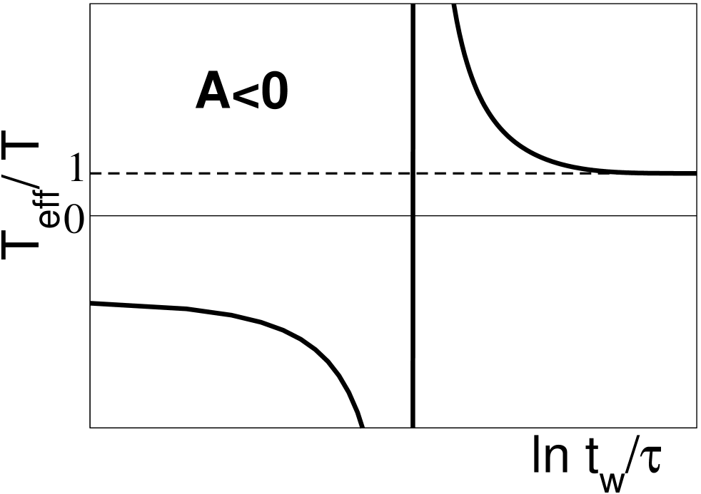
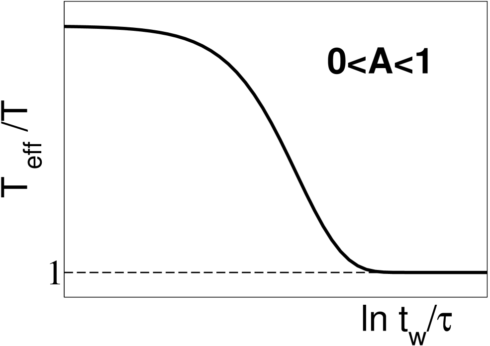
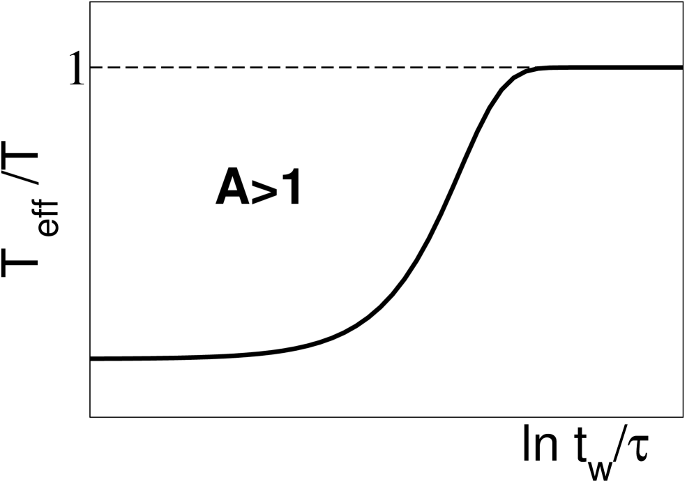
Figure 1: Qualitative behavior of $T_{eff}/T$ as a function of $t_{w}/\tau$ for $A<0$, $0<A<1$, and $A>1$.

In summary, we have shown that the origin of the violation of the FDT is the drastic elimination of variables one tacitly performs to model the system in the experimental time scale. At this level, the system evolves undergoing an activated dynamics, requiring big amounts of energy to surmount the barriers. Consequently, it is always far from equilibrium and the FDT, a result strictly valid at or near equilibrium, is not fulfilled. In the more complete scenario, when instead of jumping between two states the system reaches a different state passing progressively from intermediate configurations, i.e. diffusing in a configuration space, local equilibrium can be established. One can then proceed with the formulation of a mesoscopic nonequilibrium thermodynamics david , perfectly compatible with the Fokker-Planck level of description, whose underlying stochastic kinetics satisfies FDT. A widely-used way of quantifying the FDT violation is through the definition of an effective temperature. Our analysis shows that this concept suffers from a lack of robustness, since its value depends on the dynamical variable we measure, and can diverge or even become negative. All these problems limit the scope and question the usefulness of this quantity in the description of glassy systems where the activated dynamics is an unavoidable ingredient.

The theory we have developed provides a useful framework to describe the behavior of systems with slow dynamic bridging the macroscopic and the mesoscopic descriptions, by indicating the way to generalize local equilibrium concepts.

- (1) J.M. Rubí and C. Pérez-Vicente (eds.) Complex Behaviour of Glassy Systems, (Springer-Verlag, Berlin, 1997).
- (2) C.A.Angell, Science 267, 1924 (1995).
- (3) E. Ben-Naim, J.B. Knight, E.R. Nowak, H.M. Jaeger, S.R. Nagel, Physica D 123, 380 (1998).
- (4) P. Sollich, F. Lequeux, P. Hébreud, and M.E. Cates, Phys. Rev. Lett. 78, 2020 (1997).
- (5) K. Matan. R.B. Williams, T.A. Witten, and S.R. Nagel, Phys. Rev. Lett. 88, 076101 (2002).
- (6) L.F. Cugliandolo, J. Kurchan, Phys. Rev. Lett. 71, 173 (1997).
- (7) L.F. Cugliandolo, J. Kurchan, and L. Peliti, Phys. Rev. E 55, 3898 (1997).
- (8) J.M. Vilar, J.M. Rubí, Proc. Nat. Acad. Sci. 98, 11081 (2001).
- (9) C.A. Angell, Nature 393, 521 (1998).
- (10) P.G. Debenedetti and F.H. Stillinger, Nature 410, 259 (2001).
- (11) U. Mohanty, I. Oppenheim and C.H. Taubes, Science 266, 425 (1994).
- (12) S.R. de Groot and P. Mazur, Non-equilibrium Thermodynamics (Dover, New York, 1984).
- (13) I. Pagonabarraga, A. Pérez-Madrid and J.M. Rubí, Physica A 237, 205 (1997).
- (14) D.A. Huse and D.S. Fisher, Phys. Rev. Lett. 57, 2203 (1986).
- (15) S.A. Langer and P. Sethna, Phys. Rev. Lett. 61, 570 (1988).
- (16) P. Hänggi, P. Talkner and M. Borkovec, Rev. Mod. Phys. 62, 251 (1990).
- (17) S. A. Langer, J. P. Sethna, and R. Grannan, Phys. Rev. B 41, 2261 (1990).
- (18) R. Zwanzig, Nonequilibrium Statistical Mechanics, (University Press, Oxford, 2001).
- (19) H. Risken, The Fokker-Planck Equation (Springer, Berlin, 1989).
- (20) S. Fielding and P. Sollich, Phys. Rev. Lett 88, 050603 (2002).
- (21) L. Bellon and S. Ciliberto, to be published on Physica D, cond-mat/0201224.
- (22) L. F. Cugliandolo and J. Kurchan, J. Phys. A: Math. Gen. 27, 5749 (1994).
- (23) P. Sollich, S. Fielding, and P. Mayer, J. Phys.: Condens. Matt. 14, 1683 (2002).
- (24) K. Kawasaki, K. Fuchizaki, J. Non-Crys. Solids 235-237, 57 (1998).
- (25) A. Barrat, Phys. Rev. E 57, 3629 (1998).
- (26) L. Bellon, S. Ciliberto, and C. Laroche, Europhys. Lett. 53, 511 (2001).
- (27) T.S. Grigera and N.E. Israeloff, Phys. Rev. Lett. 83, 5038 (1999).
- (28) A. Pérez-Madrid and J.M. Rubí, Phys. Rev. E 51, 4159 (1995).
- (29) A. Pérez-Madrid, D. Reguera, and J.M. Rubí, J. Phys.: Condens. Matter 14, 1651 (2002).