A Bounded Rational Driver Model

Abstract

This paper introduces a car following model where the driving scheme takes into account the deficiencies of human decision making in a general way. Additionally, it improves certain shortcomings of most of the models currently in use: it is stochastic but has a continuous acceleration. This is achieved at the cost of formulating the model in terms of the time derivative of the acceleration, making it non-Newtonian.

To understand traffic flow, it is mandatory to analyze the interaction between the cars. The simplest case is that of a car following a lead car. To describe this process, a big number of models have been invented (for a review see Chowdhury ; Helbing ). These models differ in the details of the interaction between the cars, and the time update rule, ranging from differential equations to cellular automata. Mostly, they describe this process by an equation $a=a\left(v,h,V\right)$ that relates the change in the current velocity $v$ (the acceleration $a$) to the velocity $v$ of the following car, the distance $h$ (“headway”) to the car ahead, and its speed $V$, respectively.

Considerable effort has been invested to investigate the emerging macroscopic behavior from the underlying microscopic dynamics of interacting cars. Nevertheless, there is still a lot of controversy in both the macroscopic behavior when compared to reality daganzo-critique-sync , and in the microscopic foundations of the individual car dynamics. In particular, the observed non-damped oscillations in the relative motion of vehicles, which are illustrated in Fig. 1 are often explained by the instability in the cooperative motion of the car ensemble only (see, e.g., Chowdhury ; Helbing ). In fact, subjected to reasonable physical constraints the relation $a=a\left(v,h,V\right)$ seems to be hardly able to predict an instability in the following car motion provided the car ahead moves at a constant velocity. However, recent models BL ; Tomer ; Kerner display a certain kind of instability in the car following process itself.

There are actually two stimuli affecting the driver behavior. One of them is the necessity to move at the mean speed of traffic flow, i.e., with the speed $V$ of the leading car. So, first, the driver should control the velocity difference $v-V$. The other is the necessity to maintain a safe headway $h_{\text{opt}}(V)$ depending on the velocity $V$. In particular, the earliest “follow-the-leader” models 83 ; 84 take into account the former stimulus only without regarding the headway $h$ at all. By contrast, the “optimal velocity” model B1 ; B2 directly relates the acceleration $a$ to the difference between the current velocity $v$ and a certain optimal value $\vartheta_{\text{opt}}(h)$ at the current headway, $a\propto[v-\vartheta_{\text{opt}}(h)]$. Of course, more sophisticated approximations, e.g., Hel ; Fritz ; Xing ; skPRE ; H1 ; H2 to name but a few, allow for both stimuli.

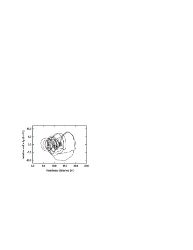
Figure 1: Measured car-following behavior. Data are recorded by an equipped car measuring distance $h$ and speed $v$ and computing $v-V$ during a drive on a German freeway.

It is not very likely that the variables $\left\{v,h,V\right\}$ do specify the acceleration $a$ completely. Since drivers have motivations and follow only partly physical regularities, memory effects may be essential. In a simple manner, this has been introduced in models that relate the current acceleration $a(t)$ to the velocity $v(t-\tau_{a})$ and the headway $h(t-\tau_{a})$ at a previous moment $t-\tau_{a}$ (for a review of the “following-the-leader” models see, e.g., Ref. D1 ; D3 , for the “optimal velocity model” see Ref. D2 ). Here, $\tau_{a}$ is the delay time in the driver response which is treated as a constant. This approach is not completely satisfactorily, since first, the physiological delay in the driver response seems to be too short to be of importance. Second, it is not clear why the memory effects relate only two moments of time instead of a certain interval as a whole. Third, the dependence of the time scale $\tau_{a}$ on the car motion state is missing. Nevertheless, these models show an instability in the car-following dynamics (provided $\tau_{a}$ is big enough) and are non-Newtonian as well.

In the following, reasons of another nature than the driver response delay lead beyond the framework of Newton’s mechanics. A corresponding model for the following car dynamics displaying an instability around the stationary motion is proposed. To describe the driver behavior, the approach suggested in Ref. we1 will be used. There, drivers plan their behavior for a certain time in advance instead of simply reacting to the surrounding situation. A similar idea related to the optimum design of a distance controlling driver assistance system is discussed in Ref. q . In mathematical terms the driver’s planning of her further motion is reduced to finding extremals of a certain priority functional that ranks outcomes of different driving strategies. Here, the assumption that the driver is rational plays the crucial role. It means that the driver continuously correct the car motion to follow the optimal strategy. In this case we2 , the collection of variables $\left\{v,h,V\right\}$ does specify the car acceleration $a$ completely. However, the assumed continuous control is impossible to achieve for humans. Therefore, it is assumed below that a real driver, first, cannot compute the optimal path of motion exactly and, second, that she cannot correct the car motion continuously.

This is just the approach that is known as bounded rationality BR1 . Even if a driver succeeds in finding the optimal solution, she is only capable of setting the acceleration to a fixed value. After that, she waits until the deviation from her priority functional has become too big to ignore, leading to a re-computation of another more or less optimal path. Or, to put it differently, drivers are simply not capable of resolving small differences between a given value of acceleration, speed, or headway and their “optimal” desired values.

The re-computations are assumed to happen stochastically, with a probability that increases with the deviation from the desired state. So, the model described below becomes a stochastic one. The action of noise can be modeled either explicitly by introducing certain thresholds (as is done in the psycho-physical models Fritz ) or by making the noise amplitude dependent on the distance between the current and optimal state. This defines a dynamic trap model we3 , an approach that will be followed below.

To make the model more realistic, it is demanded that the trajectories of acceleration, speed, and headway are continuous functions of time. This can be achieved by formulating the model in terms of the time-derivative of acceleration called jerk and adding a white-noise term there. In what follows, that the acceleration is a colorized noise process without jumps, and so are the other integrals of motion (speed and headway, respectively).

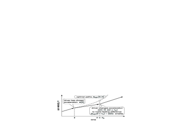
Figure 2: The driver strategy of governing the car motion.

I Model description

Assume that at a certain instant of time $t$ the driver has decided to correct the car motion and chosen the acceleration $a(t)$ (Fig. 2). As discussed above, the optimal path $\left\{\mathfrak{h}_{\text{opt}}(\mathfrak{t},t)\right\}$ of the further motion ($\mathfrak{t}>t$) is too complex for her to compute and to follow it. So, she regards the path $\left\{\mathfrak{h}_{a}(\mathfrak{t},t):\mathfrak{a}(\mathfrak{t},t)=a(t)\right\}$ characterized by the constant acceleration as the optimal one.

A certain time interval $\tau_{a}$ later, the driver has to correct the car motion again. This can be done by shifting the current acceleration $a(t+\tau_{a})$ towards the desired optimal value $a_{\text{opt}}(t+\tau_{a})=-\partial_{\mathfrak{t}}^{2}\mathfrak{h}_{\text{opt}}(\mathfrak{t},t+\tau_{a})|_{\mathfrak{t}=t+\tau_{a}}$ known to her approximately:

$$a(t+\tau_{a})-a(t)=C\left(a_{\text{opt}}(t+\tau_{a})-a(t)\right)+a_{\text{rnd}}(t+\tau_{a})\,,$$

where $C\lesssim 1$ is a constant about unity and the random term $a_{\text{rnd}}(t+\tau_{a})$ allows for the uncertainty in the driver evaluation of the optimal acceleration at the current time. Its mean amplitude $a_{c}$ characterizes physiological properties of drivers and can be considered constant. Thereby, $\left\langle a_{\text{rnd}}(t)\cdot a_{\text{rnd}}(t^{\prime})\right\rangle=a_{c}^{2}\delta_{t,t^{\prime}}$, where $\delta_{t,t^{\prime}}$ is Kronecker’s delta.

This discrete representation of the car motion correction is converted to a continuous description based on stochastic differential equations. Namely, the above discrete governing equation is reduced to

$$\frac{da}{dt}=-\frac{1}{\tau_{a}}\left(a-a_{\text{opt}}(h,v,V)\right)+\eta\xi(t)\,.$$ (1)

Here, $a_{\text{opt}}(h,v,V)$ is the optimal acceleration specified by the current values of headway, car velocity, and leading car velocity. The term $\xi(t)$ is white noise of unit amplitude which models the uncertainty in the driver evaluation of the optimal motion.

The acceleration increment $\delta a$ caused by the random force $\eta\xi(t)$ acting during the time $\tau_{a}$ is actually the random component $a_{\text{rnd}}(t)$ entering the discrete governing equation. Thus, it follows from the estimate $\langle(\delta a)^{2}\rangle\sim\eta^{2}\tau_{a}$ that

$$\eta=\frac{a_{c}}{\sqrt{\tau_{a}}}\,.$$ (2)

The time scale $\tau_{a}$ of the driver control over the car motion depends on the state $(h,v,V,a)$. Thus, the stochastic differential equation (1) contains multiplicative noise. So its type with respect to the corresponding Fokker-Planck equation has to be specified. The adopted driving strategy (Fig. 2) implies that all the characteristics of correcting the car motion are determined by its state at the “terminal” point $t+\tau_{a}$ rather than at the “initial” point $t$. Therefore, it is reasonable for Eq. (1) to be of Klimontovich type or, according to the classification in MH , to describe a “postpoint” random process.

To complete the model, $a_{\text{opt}}(h,v,V)$ and $\tau_{a}(h,v,V,a)$ have to be specified. The simple ansatz

$$a_{\text{opt}}(h,v,V)=-\frac{1}{\tau}\left[\left(v-V\right)-\frac{1}{\tau}g_{h}\left(h-h_{V}\right)\right]$$ (3)

is well justified, at least, near the stationary state of the car motion, $v=V$ and $h=h_{V}$. It should be noted that similar ideas about $a_{\text{opt}}(h,v,V)$ and a dependence of $\tau_{a}$ on the motion state had been discussed already in Ref. Hel . (See also D3 for a discussion.)

Here, $\tau$ is the characteristic time of the velocity variations and the constant $g_{h}\lesssim 1$. The limit $g_{h}\ll 1$ deserves special attention because it is just the condition that a driver, at first, prefers to eliminate the velocity difference $v-V$ between her car and the car ahead and only then optimizes the headway. In this case the optimal dynamics of car motion, i.e., the car dynamics governed by the relation $a=a_{\text{opt}}(h,v,V)$ is a pure fading relaxation towards the stationary state. Conversely, the model under consideration predicts complex oscillations in the car motion. Note, that the adopted assumption about the value of the coefficient $g_{h}$ can be justified by applying to the general principles of the car motion we2 .

If the car motion state is far from equilibrium the necessity for correcting the velocity and headway distance is obvious. In this case it is natural to suppose that the characteristic time interval $\tau_{a}$ between sequential attempts to correct the car motion should be comparable to $\tau$ which characterizes the velocity variations, i.e., $\tau_{a}\sim\tau/g_{v}$. Here, $g_{v}\gtrsim 1$ is an additional model parameter. When the car motion comes close to the equilibrium and the inequality $|a_{\text{opt}}(h,v,V)|\lesssim a_{c}$ is fulfilled the uncertainty $a_{\text{rnd}}(t+\tau_{a})$ in evaluating the optimal acceleration becomes significant. Under such conditions there is no reason for the driver to affect the car motion and she may not correct it at all. It means that the car motion control is depressed and, correspondingly, the correction time interval $\tau_{a}$ grows dramatically inside a domain $\mathbb{Q}_{u}$ of the phase plane $\left\{h,v,V\right\}$ where the inequality $|a_{\text{opt}}(h,v,V)|\lesssim a_{c}$ holds.

To compute the function $\tau_{a}(h,v,V,a)$, the boundary of the domain $\mathbb{Q}_{u}$ has to be analyzed. Note, that the acceleration itself enters the driver’s perception of motion quality: without any reason, a driver prefers not to accelerate at all. When the car motion control is active the estimate $\dot{a}\sim a/\tau_{a}$ by virtue of Eq. (1) can be adopted. So, the boundary of the domain $\mathbb{Q}_{u}$ is specified by $a^{2}_{\text{opt}}(h,v,V)+\mu^{2}a^{2}\sim a^{2}_{c}$, where $\mu\sim 1$ is a certain coefficient about unity. Assuming the variables $h$, $v$, $a$ to be independent of one another inside $\mathbb{Q}_{u}$ and averaging the latter expression over $\mathbb{Q}_{u}$ its boundary $\Phi(h,v,V,a)\sim 1$ can be derived:

$$\Phi(h,v,V,a)=\frac{\left(v-V\right)^{2}}{a_{c}^{2}\tau^{2}}+g_{h}^{2}\frac{\left(h-h_{V}\right)^{2}}{a_{c}^{2}\tau^{4}}+\mu^{2}\frac{a^{2}}{a_{c}^{2}}\,.$$ (4)

If $\Phi(h,v,V,a)\ll 1$ the driver activity in correcting the car motion is depressed completely. Otherwise, $\Phi(h,v,a)\gg 1$, the driver controls the car motion actively. This is described by the dependence of the correction time interval $\tau_{a}$ on the car motion state,

$$\frac{1}{\tau_{a}}=g_{v}\Omega\left(\Phi(h,v,V,a)\right)\frac{1}{\tau}\,.$$ (5)

The form of the function $\Omega\left(x\right)$ is illustrated in Fig. 3. Equation (1) together with expressions (2), (4), and (5) form the proposed car following model with bounded rational drivers.

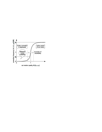
Figure 3: The correction frequency $1/\tau_{a}$ of car motion control as function of the car motion quality $\Phi(h,v,V,a)$.

When $g_{h}>g_{v}\Omega(0)$ the stationary motion with $v=V$ and $h=h_{V}$ is unstable, leading to non-damped but bounded oscillations in the headway and velocity of the following car. The particular form of the function $\Omega\left(x\right)$ is of minor importance, it is only necessary that its value inside $\mathbb{Q}_{u}$ to be small in comparison with the ratio $g_{h}/g_{v}$. When analyzing the model numerically the following ansatz

$$\Omega(x)=\exp[(x-1)/\Delta]/(\exp[(x-1)/\Delta]+1)$$

is used, with the parameter $\Delta\sim 0.2$. Below, numerical results will be presented that demonstrate the characteristic properties of the developed model.

Figure 4 displays an example of this dynamic in the $hv$-phase plane for the dimensionless headway $x=(h-h_{V})/(a_{c}\tau^{2})$ and the relative car velocity $u=(v-V)/(a_{c}\tau)$. As seen in Fig. 4, the behavior of this model is qualitatively similar to the empirical data in Fig. 1.

Preliminary results have shown that, first, the quasi-period of these oscillations in the car velocity is equal to $\tau$ times a numerical factor (about ten) depending weakly on the model parameters. For $\tau\sim 1$ s this period is similar to the observed quasi-period. Second, the amplitude of velocity oscillations does not change substantially as the model parameters vary and is about $a_{c}\tau$. By visually comparing Figs. 1, 4 the estimate $a_{c}\sim 0.3$ m/s² is obtained. It should be noted that the amplitude of the acceleration oscillations exceeds $a_{c}$ by a numerical factor about three. Third, the amplitude of the headway super-oscillations, in contrast, depends essentially on the parameter $g_{v}$, enabling one to fix this parameter based on experimental data.

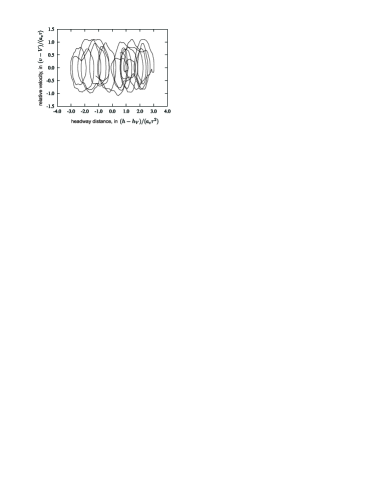
Figure 4: Simulated car-following behavior. Integration of the stochastic differential equation has been performed with the algorithms described in SRK . The parameters used are $g_{v}=5$, $g_{h}=0.2$, $\mu=1$, and $\Delta=0.2$.

II Summary

A model regarding the bounded rational behavior of car drivers has been supposed in this contribution. It takes into account that drivers, although having detailed ideas about their preferred driving strategy, are not able to control this driving strategy sufficiently precisely. Namely, drivers introduce three main sources of error into the optimal driving strategy: instead of keeping track of the changes in acceleration they simply choose a constant one, that additionally is not the optimal one but blurred by noise. This noise models the inability of drivers to evaluate exactly the very complex integrations leading to an optimal driving strategy. Therefore, the need to correct the motion from time to time arises, with the correction time intervals distributed randomly but inversely proportional to the deviation from the desired optimal acceleration.

It is shown, that these ideas can be captured in a simple model for the car-following dynamics, however at the cost of introducing a non-Newtonian term, the jerk (change in acceleration). The benefit of doing so is that the resulting model has smooth trajectories in headway, velocity and acceleration but still being a stochastic one. This discerns the approach proposed here from almost all models of car-following introduced so far.

Although the trajectories generated by this model have some similarities with real car-following data, the approach proposed here still needs thorough testing with empirical data. This will be done in the near future and will be reported soon.

These investigations were supported in part by RFBR Grants 01-01-00389, 00439 and INTAS Grant 00-0847.

References

- (1) D. Chowdhury, L. Santen, and A. Schadschneider, Phys. Rep. 329, 199 (2000).
- (2) D. Helbing, Rev. Mod. Phys. 73, 1067 (2001).
- (3) C. F. Daganzo, M. J. Cassidy and R. L. Bertini, Transp. Res. A 33, 365 (1999).
- (4) B. S. Kerner and S. L. Klenov, J. Phys. A 35, L31 (2002).
- (5) W. Knospe, L. Santen, A. Schadschneider, and M. Schreckenberg, J. Phys. A 33, L477 (2000).
- (6) E. Tomer, L. Safonov, and S. Havlin, Phys. Rev. Lett., 84, 382 (2000).
- (7) A. Reuschel, Österr. Ingen.-Archiv 4, 193 (1950).
- (8) L. A. Pipes, J. Appl. Phys. 24, 274 (1953).
- (9) M. Bando, K. Hasebe, A. Nakayama, A. Shibata, and Y. Sugiyama, Phys. Rev. E 51, 1035 (1995); Jpn. J. Ind. Appl. Math. 11, 202 (1994)
- (10) M. Bando, K. Hasebe, K. Nakanishi, A. Nakayama, A. Shibata, and Y. Sugiyama, J. Physique I 5, 1389 (1995).
- (11) W. Helly, in: Proceedings of the Symposium on Theory of Traffic Flow, Research Laboratories, General Motors (Elsevier, New York, 1959), p. 207.
- (12) H. T. Fritzsche, Transp. Eng. Contr. 5, 317 (1994).
- (13) J. Xing, in: Proceedings of the Second Word Congress on ATT, Yokohama, November, 1739 (1995).
- (14) S. Krauß, P. Wagner, and Ch. Gawron, Phys. Rev. E 55, 5597 (1997).
- (15) D. Helbing and B. Tilch, Phys. Rev. E 58, 133 (1998).
- (16) M. Treiber, M. Hennecke, and D. Helbing, Phys. Rev. E 62, 1805 (2000).
- (17) R. W. Rothery, Car Following Models, in: Traffic Flow Theory, N. Gartner, C. J. Messer, and A. K. Rathi (eds.) (Transportation Research Board, Special Report 165, 1992), Chap. 4.
- (18) M. Brackstone and M. McDonald, Trans. Res. F 2, 181 (1999).
- (19) M. Bando, K. Hasebe, K. Nakanishi, and A. Nakayama, Phys. Rev. E, 58, 5429 (1998).
- (20) I. Lubashevsky, S. Kalenkov, and R. Mahnke, Phys. Rev. E 65, 036140 (2002).
- (21) T. H. Chang and I-S. Lai, Transp. Res. C 6, 333 (1997).
- (22) I. Lubashevsky, P. Wagner, and R. Mahnke, to be published.
- (23) H. A. Simon, Theories of Bounded Rationality, in: Decision and Organization C. B. McGuire and R. Radner (eds.) (North-Holland, Amsterdam, 1972) (Chap. 8).
- (24) I. Lubashevsky, R. Mahnke, P. Wagner, and S. Kalenkov, Phys. Rev. E 66, 016117 (2002).
- (25) T. Morita and H. Hara, Physica A 101, 283 (1980); 125, 607 (1984).
- (26) K. Burrage and P. M. Burrage, Appl. Numer. Math. 22, 81 (1996).