Theory of Current and Shot Noise Spectroscopy in Single-Molecular Quantum Dots with Phonon Mode

Abstract

Using the Keldysh nonequilibrium Green function technique, we study the current and shot noise spectroscopy of a single molecular quantum dot coupled to a local phonon mode. It is found that in the presence of electron-phonon coupling, in addition to the resonant peak associated with the single level of the dot, satellite peaks with the separation set by the frequency of phonon mode appear in the differential conductance. In the “single level” resonant tunneling region, the differential shot noise power exhibit two split peaks. However, only single peaks show up in the “phonon assisted” resonant-tunneling region. An experimental setup to test these predictions is also proposed.

Recent progress in engineering and fabrication of nanoscale electronic devices has made it possible to study the transport properties of molecular devices Aviram98 ; Langlais99 ; Park00 , the linear dimension of which is at least an order smaller than semiconductor quantum dots. In addition to their potential industrial application, these devices provide an ideal test ground for the study of basic physics including the quantum size and many-body effects. The mechanism for electron conduction on such a small scale is not well understood yet. However, the evidence for quantum nature of transport properties has been observed in differential conductance for molecular wires by several experimental groups Andres96 ; Reed97 ; Kergueris99 ; Reichert02 ; Hong00 ; Rosink00 ; Chen00 ; Porath00 ; Smit02 . Theoretically, a lot of effort has been focused on the study of current-voltage characteristics of molecular wires based on either semi-empirical Tian98 ; Magoga99 ; Hall00 ; Paulsson01 ; Emberly00 or ab initio Ventra00 ; Taylor01 ; Palacios01 ; Damle02 methods. In contrast to semiconductor quantum dots, which is quite rigid in space, molecules involved in the electron tunneling process naturally possess the vibrational degrees of freedom which will inevitably react to the electron transfer through the molecules. So far, the influence of inelastic scattering process on the current-voltage characteristics of molecular wires has been considered Emberly00 while the influence on the current and its fluctuation (i.e., shot noise) has not been addressed for molecular dots. In this Letter, we use the Keldysh nonequilibrium Green function technique to calculate the current and shot noise through a single molecular quantum dot, for the first time. We focus on the effect of inelastic scattering process. A simplest Holstein-type model with a single phonon mode is employed to address the vibrational degrees of freedom in the molecular dot. All other complexity of real molecular devices, apart from interaction with phonon mode, is ignored. We find that in addition to the resonant peak associated with the single level of the dot, satellite peaks with the separation set by the frequency of phonon mode appear in the differential conductance. In the “single level” resonant tunneling region, the differential shot noise power exhibits two split peaks. However, only single peaks show up in the “phonon assisted” resonant-tunneling region. Therefore, due to the quantum nature of tunneling, the Fano factor is dramatically different from the Poisson limit even in the presence of inelastic process. These results may also be applied to the STM-based inelastic tunneling spectroscopy around a local vibrational mode on surfaces Stipe99 .

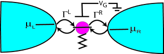
Figure 1: Schematic diagram of a molecular quantum dot system. The dot is connected to two leads with couplings $\Gamma^{L}$ and $\Gamma^{R}$. The dot electrons are also interacting with a single phonon mode. A gate electrode is capacitively attached to the dot to tune the single energy level.

The model system under consideration is illustrated in Fig. 1. It consists of a quantum dot connected with two normal conducting leads. The electrons on the dot is also coupled to a single phonon mode. The single level of the dot is tuned by a gate voltage. The system Hamiltonian is written as:

$$H=H_{L}+H_{R}+H_{X}+H_{D}+H_{T}\;.$$ (1)

The first two terms are respectively the Hamiltonian for electrons in the left and right non-interacting metallic leads:

$$H_{L}+H_{R}=\sum_{k\in L,R;\sigma}\epsilon_{k}c_{k\sigma}^{\dagger}c_{k\sigma}\;,$$ (2)

where we have denoted the electron creation (annihilation) operators in the leads by $c_{k\sigma}^{\dagger}$ ($c_{k\sigma}$). The quantity $k$ is the momentum and $\sigma$ is the spin index and $\epsilon_{k}$ is the single particle energy of conduction electrons. The third term describes the phonon mode:

$$H_{X}=\omega_{0}a^{\dagger}a\;,$$ (3)

where $\omega_{0}$ is the frequency of the single phonon mode, $a^{\dagger}$ ($a$) is phonon creation (annihilation) operator. The fourth term describes the electron in the quantum dot:

$$H_{D}=\sum_{\sigma}[\epsilon_{0}+\lambda(a+a^{\dagger})]d_{\alpha}^{\dagger}d_{\alpha}\;,$$ (4)

where $d_{\alpha}^{\dagger}$ ($d_{\alpha}$) are the creation (annihilation) operators of dot electrons, $\epsilon_{0}$ is the single energy level of the dot, $\lambda$ is the coupling constant between the dot electrons and the phonon mode. The last term represents the coupling of the dot to the leads:

$$H_{T}=\sum_{k\in L,R;\sigma,\alpha}[V_{k\sigma,\alpha}c_{k\sigma}^{\dagger}d_{\alpha}+H.c.]\;,$$ (5)

where the tunneling matrix elements $V_{k\sigma,\alpha}$ transfer electrons through an insulating barrier out of the dot.

The current operators from the leads to the dot are, respectively, defined as:

$$\hat{I}_{L(R)}=ie\sum_{k\in L(R);\sigma,\alpha}(V_{k\sigma,\alpha}c_{k\sigma}^{\dagger}d_{\alpha}-H.c.)\;.$$ (6)

The terminal current is given by $I=(\langle\hat{I}_{L}\rangle-\langle\hat{I}_{R}\rangle)/2$, where $\langle\dots\rangle$ denotes the statistical average of physical observables. Using the Keldysh nonequilibrium Green function formalism Caroli71 ; Keldysh65 , the terminal current can be obtained as Meir92 ; Jauho94 :

$$I = \frac{ie}{4\pi}\int d\epsilon\{\mbox{Tr}[(f_{L}\mathbf{\Gamma}^{L}-f_{R}\mathbf{\Gamma}^{R})(\mathbf{G}^{r}-\mathbf{G}^{a})]$$ (7)

$$+\mbox{Tr}[(\mathbf{\Gamma}^{L}-\mathbf{\Gamma}^{R})\mathbf{G}^{<}]\}\;,$$

where $f_{L(R)}$ are the Fermi distribution function of the left and right leads, which has different chemical potential upon a voltage bias $\mu_{L}-\mu_{R}=eV$, the coupling of the dot to the leads is characterized by the parameter:

$$\Gamma_{\alpha\alpha^{\prime}}^{L(R)}=2\pi\sum_{\sigma}\rho_{L(R),\sigma}(\epsilon)V_{\sigma,\alpha}^{*}(\epsilon)V_{\sigma,\alpha^{\prime}}(\epsilon)$$ (8)

with $\rho_{L(R),\sigma}$ the spin-$\sigma$ band density of states in the two leads, $G_{\alpha\alpha^{\prime}}^{r(a)}$ and $G_{\alpha\alpha^{\prime}}^{<}$, are the Fourier transform of the dot electron retarded (advanced), $G_{\alpha\alpha^{\prime}}^{r(a)}(t,t^{\prime})=\mp i\theta(\pm t\mp t^{\prime})\langle\{d_{\alpha}(t),d_{\alpha^{\prime}}^{\dagger}(t^{\prime})\}\rangle$, and lesser Green function, $G_{\alpha\alpha^{\prime}}^{<}(t,t^{\prime})=i\langle d_{\alpha^{\prime}}^{\dagger}(t^{\prime})d_{\alpha}(t)\rangle$. Note that the boldface notation indicates that the level-width function $\mathbf{\Gamma}$ and the dot electron Green functions are matrices in the spin space of dot electrons.

The electrical current through a device is fluctuating in time even under a dc bias Blanter00 . Its fluctuation is characterized by the spectral density, which is given by the Fourier transform $S(\omega)$ of the current correlation function Note1 :

$$S(t,t^{\prime})=\frac{1}{2}\langle\{\Delta\hat{I}_{L}(t),\Delta\hat{I}_{L}(t^{\prime})\}\rangle\;,$$ (9)

where $\Delta\hat{I}_{L}(t)=\hat{I}_{L}(t)-\langle\hat{I}_{L}(t)\rangle$. The quantum statistical (non-equilibrium) average involved in the current correlation can be evaluated conveniently in the Keldysh Green function formalism. Following a tedious but standard procedure, we obtain the spectral density of shot noise in the zero-frequency limit:

$$S(\omega\rightarrow 0)=\frac{e^{2}}{2\pi}\int d\epsilon\{-f_{L}(1-f_{L})(\mbox{Tr}[(\mathbf{\Gamma}^{L}\mathbf{G}^{r})^{2}]$$

$$+\mbox{Tr}[(\mathbf{\Gamma}^{L}\mathbf{G}^{a})^{2}])+if_{L}\mbox{Tr}[\mathbf{\Gamma}^{L}\mathbf{G}^{>}]-i(1-f_{L})\mbox{Tr}[\mathbf{\Gamma}^{L}\mathbf{G}^{<}]$$

$$+f_{L}\mbox{Tr}[\mathbf{\Gamma}^{L}\mathbf{G}^{>}\mathbf{\Gamma}^{L}(\mathbf{G}^{r}-\mathbf{G}^{a})]+\mbox{Tr}[\mathbf{\Gamma}^{L}\mathbf{G}^{>}\mathbf{\Gamma}^{L}\mathbf{G}^{<}]$$

$$-(1-f_{L})\mbox{Tr}[\mathbf{\Gamma}^{L}(\mathbf{G}^{r}-\mathbf{G}^{a})\mathbf{\Gamma}^{L}\mathbf{G}^{<}]\}\;,$$ (10)

where $G_{\alpha\alpha^{\prime}}^{>}$ is the Fourier transform of the greater Green function, $G_{\alpha\alpha^{\prime}}^{>}(t,t^{\prime})=-i\langle d_{\alpha}(t)d_{\alpha^{\prime}}^{\dagger}(t^{\prime})\rangle$. Equation (10) is a basic formula for the low-frequency shot noise through a quantum dot, which can take into account the many-body effects conveniently. It expresses the fluctuations of current through the quantum dot, an interacting region, in terms of the distribution functions in the leads and local properties of the quantum dot, such as the occupation and density of states. This formalism can be viewed as a generalized version of the two-terminal shot-noise formula for the non-interacting case Chen91 ; Buttiker92 , which will become clear in the following discussion. It can also be used to study the current fluctuation in the case of spin-dependent transport, which is of much interest in the study of spintronics and single spin detection.

Once the dot electron Green functions are known, the electrical current and shot noise can be calculated using Eqs. (7) and (10). In the following, we calculate these Green functions, which should be carried out in the presence of the leads. By performing a canonical transformation, $\bar{H}=e^{\mathcal{S}}He^{-\mathcal{S}}$ with $\mathcal{S}=(\lambda/\omega_{0})\sum_{\alpha}d_{\alpha}^{\dagger}d_{\alpha}(a^{\dagger}-a)$ Mahan00 , one can obtain $\bar{H}=\bar{H}_{el}+\bar{H}_{ph}$. Here $\bar{H}_{el}=\bar{H}_{L}+\bar{H}_{R}+\bar{H}_{D}+\bar{H}_{T}$ and $\bar{H}_{ph}=\bar{H}_{X}$, where $\bar{H}_{L(R)}=H_{L(R)}$, $\bar{H}_{D}=\sum_{\alpha}(\epsilon_{0}-\lambda^{2}/\omega_{0})d_{\alpha}^{\dagger}d_{\alpha}$, $\bar{H}_{T}\approx H_{T}$, and $\bar{H}_{X}=H_{X}$. Consequently, the original dot-electron Green function can be decoupled as:

$$G_{\alpha\alpha^{\prime}}^{r(a)}(t) = \mp i\theta(\pm t)\langle\{\tilde{d}_{\alpha}(t),\tilde{d}_{\alpha^{\prime}}^{\dagger}(0)\}\rangle_{el}\langle X(t)X^{\dagger}(0)\rangle_{ph}$$ (11)

$$= \tilde{G}^{r(a)}_{\alpha\alpha^{\prime}}(t)\langle X(t)X^{\dagger}(0)\rangle_{ph}\;,$$

where $\tilde{d}_{\alpha}(t)=e^{i\bar{H}_{el}t}d_{\alpha}e^{-i\bar{H}_{el}t}$, and $X(t)=e^{i\bar{H}_{ph}t}Xe^{-i\bar{H}_{ph}t}$ with $X=\exp[-(\lambda/\omega_{0})(a^{\dagger}-a)]$. The renormalization factor due to the electron-phonon interaction is evaluated to be Mahan00 : $\langle X(t)X^{\dagger}(0)\rangle_{ph}=e^{-\Phi(t)}$, where $\Phi(t)=(\lambda/\omega_{0})^{2}[N_{ph}(1-e^{i\omega_{0}t})+(N_{ph}+1)(1-e^{-i\omega_{0}t})]$ with $N_{ph}=[\exp(\beta\omega_{0})-1]^{-1}$. We then apply the equation-of-motion approach to compute the Green function $\tilde{G}_{\alpha\alpha^{\prime}}^{r(a)}$. It consists of differentiating the Green function with respect to time, thereby generating higher-order Green functions which eventually have to close (by truncation in the presence of electron-electron interaction) the equation for the Green function $\tilde{G}^{r(a)}$. A little algebra gives rise to the Fourier transform:

$$\tilde{G}_{\alpha\alpha^{\prime}}^{r(a)}(\omega)=\frac{\delta_{\alpha\alpha^{\prime}}}{\omega-(\epsilon_{0}-\Delta)-\Sigma_{\alpha\alpha}^{r(a)}}\;,$$ (12)

where the energy shift $\Delta=\lambda^{2}/\omega_{0}$ and the retarded (advanced) self-energy due to the tunneling into the electrical leads are given by:

$$\Sigma^{r(a)}_{\alpha\alpha^{\prime}}(\omega)=\sum_{k\in L,R}\frac{|V_{k\alpha,\alpha}|^{2}\delta_{\alpha\alpha^{\prime}}}{\omega-\epsilon_{k}\pm i0^{+}}\;.$$ (13)

The full width of the resonance is then just the sum of elastic couplings to the two leads which is given by Eq. (8). The Fourier transform of the full Green function given by Eq. (11) can be obtained as:

$$G_{\alpha\alpha^{\prime}}^{r(a)} = e^{-g(2N_{ph}+1)}\sum_{l=-\infty}^{\infty}J_{l}(2g\sqrt{N_{ph}(N_{ph}+1)})$$ (14)

$$\times\frac{\delta_{\alpha\alpha^{\prime}}e^{l\omega_{0}\beta/2}}{\omega-(\epsilon_{0}-\Delta)-l\omega_{0}-\Sigma_{\alpha\alpha}^{r(a)}}\;,$$

where $J_{l}(x)$ are the Bessel functions of complex argument, the parameter $g=(\lambda/\omega_{0})^{2}$. The Green function $G_{\alpha\alpha^{\prime}}^{<(>)}$ cannot be obtained by directly using the above equation-of-motion approach. By instead applying the operational rules as given by Langreth Langreth76 to the Dyson equation for the contour-ordered Green function, one can show the following Keldysh equation for the lesser and greater functions Jauho94 : $\mathbf{G}^{<(>)}(\omega)=\mathbf{G}^{r}(\omega)\mathbf{\Sigma}^{<(>)}_{T}(\omega)\mathbf{G}^{a}(\omega)\;.$ In the weak electron-phonon coupling limit as we are considering here, the contribution to the self-energy $\mathbf{\Sigma}_{T}^{<(>)}$ from the electron-phonon interaction is negligible such that $\mathbf{\Sigma}_{T}^{<(>)}$ can be approximated by the lesser (greater) self-energy due to the tunneling into the two leads: $\mathbf{\Sigma}^{<}=i[f_{L}\mathbf{\Gamma}^{L}+f_{R}\mathbf{\Gamma}^{R}]\;,$ and $\mathbf{\Sigma}^{>}=-i[(1-f_{L})\mathbf{\Gamma}^{L}+(1-f_{R})\mathbf{\Gamma}^{R}]\;.$ This relation enables us to rewrite the current and shot noise formulae as:

$$I=\frac{e}{2\pi}\int d\epsilon[f_{L}-f_{R}]\mbox{Tr}[\mathbf{T}]\;,$$ (15)

and

$$S = \frac{e^{2}}{2\pi}\int d\epsilon\{[f_{L}(1-f_{L})+f_{R}(1-f_{R})]\mbox{Tr}[\mathbf{T}]$$ (16)

$$+(f_{L}-f_{R})^{2}\mbox{Tr}[(1-\mathbf{T})\mathbf{T}]\}\;,$$

where we have defined the transmission coefficient matrix $\mathbf{T}=\mathbf{G}^{a}\mathbf{\Gamma}^{L}\mathbf{G}^{r}\mathbf{\Gamma}^{R}$. We remark that for the noninteracting case (no electron-phonon and electron-electron interactions), the above two expressions are exact. These are just the Landauer-Büttiker formalisms developed for the noninteracting electron transport based on the scattering matrix theory. The connection between the two formalisms for the current was first established by Meir and Wingreen Meir92 .

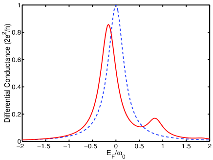
Figure 2: Differential conductance, in units of $2e^{2}/h$, through the molecular quantum dot as a function of the Fermi energy $E_{F}$ measured relative to the single level of the quantum dot in the presence (red-solid line, $\lambda=0.4\omega_{0}$) and absence (blue-dashed line, $\lambda=0$) of electron-phonon coupling. The energy is measured in units of the frequency of the phonon mode $\omega_{0}$, and $\Gamma^{L}=\Gamma^{R}=0.2\omega_{0}$.

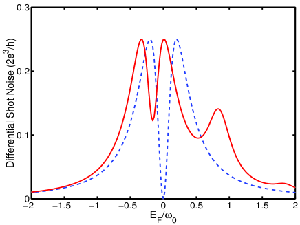
Figure 3: Differential shot noise power, in units of $2e^{3}/h$, through the molecular quantum dot as a function of the Fermi energy $E_{F}$ measured relative to the single level of the quantum dot in the presence (red-solid line, $\lambda=0.4\omega_{0}$) and absence (blue-dashed line, $\lambda=0$) of electron-phonon coupling. The energy is measured in units of the frequency of the phonon mode $\omega_{0}$, and $\Gamma^{L}=\Gamma^{R}=0.2\omega_{0}$.

For simplicity, we consider the coupling of the dot to the two leads to be symmetric $\mathbf{\Gamma^{L}}=\mathbf{\Gamma}^{R}$, and assume that the leads have broad and flat density of states (i.e., the wideband limit). For this case, the elastic couplings, from which the self-energy (13) can be determined, are independent of energy. In Figs. 2 and 3, we plot the zero-temperature differential conductance and shot noise power as a function of the Fermi energy (that is, the equilibrium chemical potential in the leads) measured relative to the single level $\epsilon_{0}$ in the presence (with typical value $\lambda=0.4\omega_{0}$, red-solid lines in the figures) and absence ($\lambda=0$, blue-dashed lines) of electron-phonon coupling. Here all energy quantities are measured in units of the phonon mode frequency $\omega_{0}$, and the elastic couplings $\Gamma^{L}=\Gamma^{R}$ are fixed at $0.2\omega_{0}$. When the electron is not coupled to the phonon mode, only one resonant conductance peak shows up as the Fermi energy matches the single level in the quantum dot. In the presence of electron-phonon coupling, the overall spectrum is shifted by $\Delta=\lambda^{2}/\omega_{0}$. In addition to the main peak related to the single level, new satellite resonant peaks appear at the positive energy side. The separation between the conductance peaks is set by the frequency of the phonon mode $\omega_{0}$. Since at zero temperature no phonon modes are excited on the quantum dot, the electrons tunneling onto the dot can only excite phonon modes, which explains why the satellite peaks are located at the positive energy region. It can be expected that there will appear satellite peaks at negative energy region at finite temperatures, where thermally excited phonons can be absorbed by the electrons tunneling onto the dot. Moreover, the intensity of the satellite peaks is much smaller than the main resonant peak because they are evolving from the emission of phonon modes, which is controlled by the electron-phonon coupling. Correspondingly, the differential shot noise power exhibits two peaks located symmetrically around the position where the conductance peak associated with the single level of the dot is located. The origin of this behavior is that no noise is generated when the transmission probability $T=0$ or $1$, while it is generated maximally in between. In this “single level” resonant-tunneling region, the Fano factor defined as the ratio of shot noise to current is significantly enhanced. Since the transmission probability corresponding to those satellite conductance peaks (from the phonon emission process) is small, the differential noise power is approximately proportional to the conductance and only show a single peak rather than two peaks. Therefore, in the “phonon assisted” resonant-tunneling region, the Fano factor is smaller than one, in contrast to the case of “single level” resonant tunneling. Therefore, due to the quantum tunneling nature, the Fano factor for the present system differs the Poisson limit (equal to 2), where electrons diffuse in an uncorrelated way.

To experimentally investigate the current and shot noise spectroscopy of molecular quantum dots, we suggest a setup where a gate electrode is attached to the dot capacitively, as shown in Fig. 1. A gate voltage is applied solely to tune the level position on the dot while a bias voltage is applied in the linear response regime. The merit of the proposed setup is that the internal electronic and ionic charge buildup on the dot, which is generated by a nonlinear response, could be avoided safely. Experimental effort along this direction is in progress Park02 .

To summarize, using the Keldysh nonequilibrium Green function technique, we have studied in this work, to the best of our knowledge, for the first time the current and shot noise spectroscopy of a single molecular quantum dot coupled to a local phonon mode. We show that, in the presence of electron-phonon coupling, in addition to the resonant peak associated with the single level of the dot, satellite peaks with the separation set by the frequency of phonon mode appear in the differential conductance. In the “single level” resonant tunneling region, the differential shot noise power exhibits two split peaks. However, only single peaks show up in the “phonon assisted” resonant-tunneling region. The Fano factor is different from the Poisson limit even in the presence of inelastic process. The derived current and noise formalism can also be applied to more complicated systems.

Acknowledgments: We thank A. Abanov and R. Lu for useful discussions. This work was supported by the Department of Energy.

References

- (1) A. Aviram and M. Ratner, eds., Molecular Electronics: Science and Technology (Annals of the New York Academy of Sciences, New York, 1998).
- (2) V. Langlais et al., Phys. Rev. Lett. 83, 2809 (1999).
- (3) H. Park et al., Nature 407, 57 (2000).
- (4) R. P. Andres et al., Science 272, 1323 (1996).
- (5) M. A. Reed et al., Science 278, 252 (1997).
- (6) C. Kergueris et al., Phys. Rev. B 59, 12505 (1999).
- (7) J. Reichert et al., Phys. Rev. Lett. 88, 176804 (2002).
- (8) S. Hong et al., Superlatt. and Microstruc. 28, 289 (2000).
- (9) J. J. W. Rosink et al., Phys. Rev. B 62, 10459 (2000).
- (10) J. Chen et al., Appl. Phys. Lett. 77, 1224 (2000).
- (11) D. Porath et al., Nature 403, 635 (2000).
- (12) R. H. M. Smit et al., cond-mat/0208407.
- (13) W. Tian et al., J. Chem. Phys. 109, 2874 (1998).
- (14) M. Magoga and C. Joachim, Phys. Rev. B 59, 16011 (1999).
- (15) L. E. Hall et al., J. Chem. Phys. 112, 1510 (2000).
- (16) M. Paulsson and S. Stafström, Phys. Rev. B 64, 035416 (2001).
- (17) E. G. Emberly and G. Kirczenow, Phys. Rev. B 62, 10451 (2000).
- (18) M. Di Ventra, S. T. Pantelides, and N. D. Lang, Phys. Rev. Lett. 84, 979 (2000).
- (19) J. Taylor, H. Gou, and J. Wang, Phys. Rev. B 63, 245407 (2001).
- (20) J. J. Palacios et al., Phys. Rev. B 64, 115411 (2001).
- (21) P. S. Damle, A. W. Ghosh, and S. Datta, Chem. Phys. 281, 171 (2002).
- (22) B. C. Stipe, M. A. Rezaei, and W. Ho, Science 280, 1732 (1998); Phys. Rev. Lett. 82, 1724 (1999); N. Lorente et al., ibid. 86, 2593 (2001).
- (23) C. Caroli et al., J. Phys. C 4, 916 (1971).
- (24) L. V. Keldysh, Zh. Eksp. Teor. Fiz. 47, 1515 (1965) [Sov. Phys. JETP 20, 1018 (1965).
- (25) Y. Meir and N. S. Wingreen, Phys. Rev. Lett. 68, 2512 (1992).
- (26) A.-P. Jauho, N. S. Wingreen, and Y. Meir, Phys. Rev. B 50, 5528 (1994).
- (27) For a review, see, Ya. M. Blanter and M. Büttiker, Phys. Rep. 336, 1 (2000).
- (28) For the case of a quantum dot connected to two leads, the current conservation requires that . Therefore, the current fluctuations are the same at either lead, and they have the opposite sign with the correlation of fluctuations at two leads, i.e., . It is then sufficient for us to calculate the current correlation at the left lead.
- (29) L. Y. Chen and C. S. Ting, Phys. Rev. B 43, 4534 (1991).
- (30) M. Büttiker, Phys. Rev. B 46, 12485 (1992); Phys. Rev. Lett. 65, 2901 (1990).
- (31) G. D. Mahan, Many-Particle Physics, 3rd ed. (Plenum Press, New York, 2000).
- (32) D. C. Langreth, in Linear and Nonlinear Electron Transport in Solids, edited by J. T. Devreese and V. E. Van Doren (Plenum, New York, 1976).
- (33) J. Park et al., ibid. 417, 722 (2002); W. Liang et al., ibid. 417, 725 (2002).