Corollary to the Hohenberg-Kohn Theorem

Abstract

According to the Hohenberg-Kohn theorem, there is an invertible one-to-one relationship between the Hamiltonian $\hat{H}$ of a system and the corresponding ground state density $\rho({\bf r})$. The extension of the theorem to the time-dependent case by Runge and Gross states that there is an invertible one-to-one relationship between the density $\rho({\bf r}t)$ and the Hamiltonian $\hat{H}(t)$. In the proof of the theorem, Hamiltonians $\hat{H}/\hat{H}(t)$ that differ by an additive constant $C$/ function $C(t)$ are considered equivalent. Since the constant $C$/ function $C(t)$ is extrinsically additive, the physical system defined by these differing Hamiltonians $\hat{H}/\hat{H}(t)$ is the same. Thus, according to the theorem, the density $\rho({\bf r})/\rho({\bf r}t)$ uniquely determines the physical system as defined by its Hamiltonian $\hat{H}/\hat{H}(t)$. Hohenberg-Kohn, and by extension Runge and Gross, did not however consider the case of a set of degenerate Hamiltonians $\{\hat{H}\}/\{\hat{H}(t)\}$ that differ by an intrinsic constant $C$/function $C(t)$ but which represent different physical systems and yet possess the same density $\rho({\bf r})/\rho({\bf r}t)$ . The intrinsic constant C/function C(t) contains information about the different physical systems and helps differentiate between them. In such a case, the density $\rho({\bf r})/\rho({\bf r}t)$ cannot distinguish between these different Hamiltonians. In this paper we construct such a set of degenerate Hamiltonians $\{\hat{H}\}/\{\hat{H}(t)\}$. Thus, although the proof of the Hohenberg-Kohn theorem is independent of whether the constant $C$/function $C(t)$ is additive or intrinsic, the applicability of the theorem is restricted to excluding the case of the latter. The corollary is as follows: Degenerate Hamiltonian $\{\hat{H}\}/\{\hat{H}(t)\}$ that represent different physical systems, but which differ by a constant $C$/function $C(t)$ , and yet possess the same density $\rho({\bf r})/\rho({\bf r}t)$, cannot be distinguished on the basis of the Hohenberg-Kohn/Runge-Gross theorem.

I I. Introduction and Corollary

This paper provides further insight into the first of the two Hohenberg-Kohn (HK) theorems 1 that constitute the rigorous mathematical basis for density functional theory. According to the theorem, for a system of $N$ electrons in an external field $\mathcal{F}^{ext}({\bf r})=-{\bf\nabla}v({\bf r})$, the ground state electronic density $\rho({\bf r})$ for a nondegenerate state determines the external potential energy $v({\bf r})$ uniquely to within an unknown trivial additive constant $C$. Since the kinetic energy $\hat{T}$ and electronic-interaction potential energy $\hat{U}$ operators are known, the Hamiltonian $\hat{H}$ is explicitly known. The solutions $\Psi$ of the corresponding time-independent Schrödinger equation, for both ground and excited states, then determine the properties of the electronic system. The wave function is thus a functional of the density: $\Psi=\Psi[\rho]$, and therefore all expectations are unique functionals of the density. Thus, the ground state density $\rho({\bf r})$ determines all the properties of the system.

In the extension of the first HK theorem to the time-dependent case, Runge and Gross(RG) 2 prove that for a system of $N$ electrons in a time-dependent external field $\mathcal{F}^{ext}({\bf r}t)=-{\bf\nabla}v({\bf r}t)$, such that the potential energy $v({\bf r}t)$ is Taylor- expandable about some initial time $t_{0}$, the density $\rho({\bf r}t)$ evolving from some fixed initial state $\Psi(t_{0})$, determines the external potential energy uniquely to within an additive purely time-dependent function $C(t)$. Again, as the kinetic and electron-interaction potential energy operators are already defined, the Hamiltonian ${\hat{H}}(t)$ is known. The solution $\Psi(t)$ of the time-dependent Schrödinger equation then determines the system properties. Equivalently, the wave function $\Psi(t)$ is a functional of the density, unique to within a time-dependent phase. As such all expectation values are unique functionals of the density, the phase factor cancelling out.

In the preamble to their proof, HK/RG consider Hamiltonians $\hat{H}/\hat{H}(t)$ that differ by an additive constant $C$/function $C(t)$ to be equivalent. In other words, the physical system under consideration as defined by the electronic Hamiltonian remains the same on addition of this constant/function which is arbitrary. Thus, measurement of properties of the system, other than for example the total energy $E/E(t)$, remain invariant. The theorem then proves that each density $\rho({\bf r})/\rho({\bf r}t)$ is associated with one and only one Hamiltonian $\hat{H}/\hat{H}(t)$ or physical system: the density $\rho({\bf r})/\rho({\bf r}t)$ determines that unique Hamiltonian $\hat{H}/\hat{H}(t)$ to within an additive constant $C$/function $C(t)$.

HK/RG, however, did not consider the case of a set of Hamiltonians $\{\hat{H}\}/\{\hat{H}(t)\}$ that represent different physical systems which differ by an intrinsic constant $C$/function $C(t)$, but which yet have the same density $\rho({\bf r})/\rho({\bf r}t)$. By intrinsic constant $C$/function $C(t)$ we mean one that is inherent to the system and not extrinsically additive. Thus, this constant $C$/function $C(t)$ helps distinguish between the different Hamiltonians in the set $\{\hat{H}\}/\{\hat{H}(t)\}$, and is consequently not arbitrary. That the physical systems are different could, of course, be confirmed by experiment. Further, the density $\rho({\bf r})/\rho({\bf r}t)$ would then not be able to distinguish between the different Hamiltonians $\{\hat{H}\}/\{\hat{H}(t)\}$ or physical systems, as it is the same for all of them.

In this paper we construct a set of model systems with different Hamiltonians $\{\hat{H}\}/\{\hat{H}(t)\}$ that differ by a constant $C$/function $C(t)$ but which all possess the same density $\rho({\bf r})/\rho({\bf r}t)$. This is the Hooke’s species: atom, molecule, all positive molecular ions with number of nuclei $\mathcal{N}$ greater than two. The constants $C$/function $C(t)$ contain information about the system, and are intrinsic to distinguishing between the different elements of the species.

The corollary to the HK/RG theorem is as follows: Degenerate Hamiltonians $\{\hat{H}\}/\{\hat{H}(t)\}$ that differ by a constant $C$/function $C(t)$ but which represent different physical systems all possessing the same density $\rho({\bf r})/\rho({\bf r}t)$ cannot be distinguished on the basis of the HK/RG theorem. That is, for such systems, the density $\rho({\bf r})/\rho({\bf r}t)$ cannot determine each external potential energy $v({\bf r})/v({\bf r}t)$, and hence each Hamiltonian of the set $\{\hat{H}\}/\{\hat{H}(t)\}$, uniquely.

In the following sections, we describe the Hooke’s species for the time-independent and time-dependent cases to prove the above corollary.

II II. HOOKE’S SPECIES

A.  Time-Independent case.

Prior to describing the Hooke’s species, let us consider the following Coulomb species of two-electron systems and $\mathcal{N}$ nuclei: the Helium atom ($\mathcal{N}=1$; atomic number $Z=2$), the Hydrogen molecule ($\mathcal{N}=2$; atomic number of each nuclei $Z=1$), and the positive molecular ions ($\mathcal{N}>2$; atomic number of each nuclei $Z=1$).

In atomic units, the Hamiltonian of the Coulomb species is

$$\hat{H}_{\mathcal{N}}=\hat{T}+\hat{U}+\hat{V}_{\mathcal{N}}$$ (1)

where $\hat{T}$ is the kinetic energy operator:

$$\hat{T}=-\frac{1}{2}\sum^{2}_{i=1}{\nabla_{i}}^{2},$$ (2)

$\hat{U}$ the electron-interaction potential energy operator:

$$\hat{U}=\frac{1}{|{\bf r}_{1}-{\bf r}_{2}|},$$ (3)

and $\hat{V}_{\mathcal{N}}$ the external potential energy operator:

$$\hat{V}_{\mathcal{N}}=\sum^{2}_{i=1}v_{\mathcal{N}}({\bf r}_{i}),$$ (4)

with

$$v_{\mathcal{N}}({\bf r})=\sum^{\mathcal{N}}_{j=1}f_{C}({\bf r}-{\bf R}_{j}).$$ (5)

where

$$f_{C}({\bf r}-{\bf R}_{j})=-\frac{1}{|{\bf r}-{\bf R}_{j}|}.$$ (6)

Here ${\bf r}_{1}$ and ${\bf r}_{2}$ are positions of the electrons, ${\bf R}_{j}(j=1,...\mathcal{N})$ the positions of the nuclei, and $f_{C}({\bf r}-{\bf R}_{j})$ the Coulomb external potential energy function. Each element of the Coulomb species represents a different physical system. ( The species could be further generalized by requiring each nuclei to have a different charge.)

Now suppose the ground state density $\rho({\bf r})$ of the Hydrogen molecule were known. Then, according to the HK theorem, this density uniquely determines the external potential energy operator to within an additive constant $C$:

$${\hat{V}}_{\mathcal{N}=2}=-\frac{1}{|{\bf r}_{1}-{\bf R}_{1}|}-\frac{1}{|{\bf r}_{1}-{\bf R}_{2}|}-\frac{1}{|{\bf r}_{2}-{\bf R}_{1}|}-\frac{1}{|{\bf r}_{2}-{\bf R}_{2}|}.$$ (7)

Thus, the Hamiltonian of the Hydrogen molecule is exactly known from the ground state density. Note that in addition to the functional form of the external potential energy, the density also explicitly defines the positions ${\bf R}_{1}$ and ${\bf R}_{2}$ of the nuclei.

The fact that the ground state density determines the external potential energy operator, and hence the Hamiltonian may be understood as follows. Integration of the density leads to the number $N$ of the electrons: $\int\rho({\bf r})d{\bf r}=N$. The cusps in the electron density which satisfies the electron-nucleus cusp condition 3 , determine in turn the positions of the $\mathcal{N}$ nuclei and their charge $Z$. Thus, the external potential energy operator ${\hat{V}}_{\mathcal{N}}=\sum_{i}v_{\mathcal{N}}({\bf r}_{i})$, and therefore the Hamiltonian ${\hat{H}}$ are known.

The Hooke’s species comprise of two electrons coupled harmonically to a variable number $\mathcal{N}$ of nuclei. The electrons are coupled to each nuclei with a different spring constants $k_{j},j=1...\mathcal{N}$. The species comprise of the Hooke’s atom ($\mathcal{N}=1$, atomic number $Z=2$, spring constant k), the Hooke’s molecule ($\mathcal{N}=2$; atomic number of each nuclei $Z=1$, spring constants $k_{1}$ and $k_{2}$), and the Hooke’s positive molecular ions ($\mathcal{N}>2$, atomic number of each nuclei $Z=1$, spring constants $k_{1},k_{2},k_{3}...k_{\mathcal{N}}$). The Hamiltonian ${\hat{H}}_{\mathcal{N}}$ of this species is the same as that of the Coulomb species of Eq.(1) except that the external potential energy function is $f_{H}({\bf r}-{\bf R}_{j})$, where

$$f_{H}({\bf r}-{\bf R}_{j})=\frac{1}{2}k_{j}({\bf r}-{\bf R}_{j})^{2}.$$ (8)

Just as for the Coulomb species, each element of the Hooke’s species represents a different physical system. Thus, for example, the Hamiltonian for Hooke’s atom is

$$\hat{H}_{a}=-\frac{1}{2}{\nabla_{1}}^{2}-\frac{1}{2}{\nabla_{2}}^{2}+\frac{1}{|{\bf r}_{1}-{\bf r}_{2}|}+\frac{1}{2}k[({\bf r}_{1}-{\bf R}_{1})^{2}+({\bf r}_{2}-{\bf R}_{1})^{2}],$$ (9)

and that of Hooke’s molecule is

$$\hat{H}_{m}=-\frac{1}{2}{\nabla_{1}}^{2}-\frac{1}{2}{\nabla_{2}}^{2}+\frac{1}{|{\bf r}_{1}-{\bf r}_{2}|}+\frac{1}{2}\{k_{1}[({\bf r}_{1}-{\bf R}_{1})^{2}+({\bf r}_{2}-{\bf R}_{1})^{2}]+k_{2}[({\bf r}_{1}-{\bf R}_{2})^{2}+({\bf r}_{2}-{\bf R}_{2})^{2}]\},$$ (10)

where $k\neq k_{1}\neq k_{2}$, and so on for the various Hooke’s positive molecular ions with $\mathcal{N}>2$.

For the Hooke’s species, however, the external potential energy operator ${\hat{V}}_{\mathcal{N}}$ which is

$${\hat{V}}_{\mathcal{N}}=\frac{1}{2}\sum^{\mathcal{N}}_{j=1}[k_{j}({\bf r}_{1}-{\bf R}_{j})^{2}+k_{j}({\bf r}_{2}-{\bf R}_{j})^{2}],$$ (11)

may be rewritten as

$${\hat{V}}_{\mathcal{N}}=(\frac{1}{2}\sum^{\mathcal{N}}_{j=1}k_{j})[({\bf r}_{1}-{\bf a})^{2}+({\bf r}_{2}-{\bf a})^{2}]+C(\{k\},\{{\bf R}\},\mathcal{N}),$$ (12)

where the translation vector ${\bf a}$ is

$${\bf a}=\sum^{\mathcal{N}}_{j=1}k_{j}{\bf R}_{j}/\sum^{\mathcal{N}}_{j=1}k_{j},$$ (13)

and the constant $C$ is

$$C=b-d$$ (14)

with

$$b=\sum^{\mathcal{N}}_{j=1}k_{j}{\bf R}_{j}^{2},$$ (15)

$$d=(\sum^{\mathcal{N}}_{j=1}k_{j}{\bf R}_{j})^{2}/\sum^{\mathcal{N}}_{j=1}k_{j},$$ (16)

or

$$C=\frac{1}{2}\sum^{\mathcal{N}}_{i,j=1}{{}^{\prime}}k_{i}k_{j}({\bf R}_{i}-{\bf R}_{j})^{2}/\sum^{\mathcal{N}}_{j=1}k_{j}.$$ (17)

From Eq.(12) it is evident that the Hamiltonians ${\hat{H}}_{\mathcal{N}}$ of the Hooke’s species are those of a Hooke’s atom ($\sum^{\mathcal{N}}_{j=1}k_{j}=k$), (to within a constant $C(\{k\},\{{\bf R}\},\mathcal{N})$), whose center of mass is at ${\bf a}$. The constant $C$ which depends upon the spring constants $\{k\}$, the positions of the nuclei $\{{\bf R}\}$, and the number $\mathcal{N}$ of the nuclei, differs from a trivial additive constant in that it is an intrinsic part of each Hamiltonian ${\hat{H}}_{\mathcal{N}}$, and distinguishes between the different elements of the species. It does so because the constant $C(\{k\},\{\bf R\},\mathcal{N})$ contains physical information about the system such as the positions $\{\bf R\}$ of the nuclei.

Now according to the HK theorem, the ground state density determines the external potential energy, and hence the Hamiltonian, to within a constant. Since the density of each element of the Hooke’s species is that of the Hooke’s atom, it can only determine the Hamiltonian of a Hooke’s atom and not the constant $C(\{k\},\{{\bf R}\},\mathcal{N})$. Therefore, it cannot determine the Hamiltonian ${\hat{H}}_{\mathcal{N}}$ for $\mathcal{N}>1$. This is reflected by the fact that the density of the elements of the Hooke’s species does not satisfy the electron-nucleus cusp condition.( It is emphasized that although the ‘degenerate Hamiltonians’ of the Hooke’s species have a ground state wave function and density that corresponds to that of a Hooke’s atom, each element of the species represents a different physical system. Thus, for example, a neutron diffraction experiment on the Hooke’s molecule and Hooke’s positive molecular ion would all give different results).

It is also possible to construct a Hooke’s species such that the density of each element is the same. This is most readily seen for the case when the center of mass is moved to the origin of the coordinate system, i.e. for ${\bf a}=0$. This requires, from Eq.(13), the product of the spring constants and the coordinates of the nuclei satisfy the condition

$$\sum^{\mathcal{N}}_{j=1}k_{j}{\bf R}_{j}=0,$$ (18)

so that the external potential energy operator is then

$${\hat{V}}_{\mathcal{N}}({\bf r})=\frac{1}{2}\sum^{\mathcal{N}}_{j=1}k_{j}{\bf r}^{2}+\frac{1}{2}\sum^{\mathcal{N}}_{j=1}k_{j}{\bf R}_{j}^{2},$$ (19)

where ${\bf r}$ is the distance to the origin. If the sum $\sum^{\mathcal{N}}_{j=1}k_{j}$ is then adjusted to equal a particluar value of the spring constant $k$ of Hooke’s atom:

$$\sum^{\mathcal{N}}_{j=1}k_{j}=k,$$ (20)

then the Hamiltonian ${\hat{H}}_{\mathcal{N}}$ of any element of the species may be rewritten as

$${\hat{H}}_{\mathcal{N}}(\{k\},\{{\bf R}\},\mathcal{N})={\hat{H}}_{a}(k)+C(\{k\},\{{\bf R}\},\mathcal{N}),$$ (21)

where ${\hat{H}}_{a}(k)$ is the Hooke’s atom Hamiltonian and the constant $C(\{k\},\{\bf R\},\mathcal{N})$ is

$$C(\{k\},\{{\bf R}\},\mathcal{N})=\sum^{\mathcal{N}}_{j=1}k_{j}{\bf R}_{j}^{2}.$$ (22)

The solution of the Schrödinger equation and the corresponding density for each element of the species are therefore the same.

As an example, again consider the case of Hooke’s atom and molecule. For Hooke’s atom $\mathcal{N}=1,{\bf R}_{1}=0$, and let us assume $k=\frac{1}{4}$. Thus, the external potential energy operator is

$$v_{a}({\bf r})=\frac{1}{2}kr^{2}=\frac{1}{8}r^{2}.$$ (23)

For this choice of $k$, the singlet ground state solution of the time-independent Schrödinger equation $(\hat{H}_{\mathcal{N}}\Psi=E_{\mathcal{N}}\Psi)$ is analytical 4 :

$$\Psi({\bf r}_{1}{\bf r}_{2})=De^{-y^{2}/2}e^{-r^{2}/8}(1+r/2),$$ (24)

where ${\bf r}={\bf r}_{1}-{\bf r}_{2},{\bf y}=({\bf r}_{1}+{\bf r}_{2})/2$, and $D=1/[2\pi^{5/4}(5\sqrt{\pi}+8)^{1/2}]$. The corresponding ground state density $\rho({\bf r})=\langle\Psi|\hat{\rho}({\bf r})|\Psi\rangle$, $\hat{\rho}({\bf r})=\sum^{2}_{i=1}\delta({\bf r}-{\bf r}_{i})$ is 5 ; 6

$$\rho({\bf r})=\frac{\pi\sqrt{2\pi}}{r}D^{2}e^{-r^{2}/2}\{7r+r^{3}+(8/\sqrt{2\pi})re^{-r^{2}/2}+4(1+r^{2})erf(r/\sqrt{2}\},$$ (25)

where

$$erf(x)=\frac{2}{\sqrt{\pi}}\int^{x}_{0}e^{-z^{2}}dz.$$ (26)

For the Hooke’s molecule, $\mathcal{N}=2,{\bf R}_{1}=-{\bf R}_{2}$, and we choose $k_{1}=k_{2}=\frac{1}{8}$, so that the external potential energy operator is

$$v_{m}({\bf r})=\frac{1}{8}r^{2}+\frac{1}{16}(R_{1}^{2}+R_{2}^{2})=\frac{1}{8}r^{2}+\frac{1}{8}R^{2},$$ (27)

where $|{\bf R}_{1}|=R$. Thus, the Hamiltonian for Hooke’s molecule differs from that of Hooke’s atom by only the constant $\frac{1}{8}R^{2}$, thereby leading to the same ground state wave function and density. However, the ground state energy of the two elements of the species differ by $\frac{1}{8}R^{2}$.

The above example demonstrating the equivalence of the density of the Hooke’s atom and molecule is for a specific value of the spring constant $k$ for which the wave function happens to be analytical. However, this conclusion is valid for arbitrary value of $k$ for which solutions of the Schrödinger equation exist but are not necessarily analytical. For example, if we assume that for each element of the species ($\mathcal{N}\geq 2$), all the spring constants $k_{j},j=1,2,...\mathcal{N}$ are the same and designated by $k^{\prime}$, then for the three values of $k$ for the Hooke’s atom corresponding to $k=\frac{1}{4},\frac{1}{2},1$, the values of $k^{\prime}$ for which the Hooke’s molecule and molecular ion ($\mathcal{N}=3$) wave functions are the same are $k^{\prime}=\frac{1}{8},\frac{1}{12};\;k^{\prime}=\frac{1}{4},\frac{1}{6};\;k^{\prime}=\frac{1}{2},\frac{1}{3}$, respectively.

Thus, for the case where the elements of the Hooke’s species are all made to have the same ground state density $\rho({\bf r})$, the density cannot, on the basis of the HK theorem, distinguish bewteen the different physical elements of the species.

Corollary: Degenerate time-independent Hamiltonians $\{{\hat{H}}\}$ that represent different physical systems, but which differ by a constant $C$ , and yet possess the same density $\rho({\bf r})$, cannot be distinguished on the basis of the Hohenberg-Kohn theorem.

B.  Time-Dependent case.

We next extend the above conclusions to the time-dependent HK theorem. Consider again the Hooke’s species, but in this case let us assume that the positions of the nuclei are time-dependent, i.e. ${\bf R}_{j}={\bf R}_{j}(t)$. This could represent, for example, the zero point motion of the nuclei. For simplicity we consider the spring constant strength to be the same ($k^{\prime}$) for interaction with all the nuclei. The external potential energy $v_{\mathcal{N}}({\bf r}t)$ for an arbitrary member of the species which now is

$$v_{\mathcal{N}}({\bf r}t)=\frac{1}{2}k^{\prime}\sum^{\mathcal{N}}_{j=1}({\bf r}-{\bf R}_{j}(t))^{2},$$ (28)

may then be rewritten as

$$v_{\mathcal{N}}({\bf r}t)=\frac{1}{2}\mathcal{N}k^{\prime}r^{2}-k^{\prime}\sum^{\mathcal{N}}_{j=1}{\bf R}_{j}(t)\cdot{\bf r}+\frac{1}{2}k^{\prime}\sum^{\mathcal{N}}_{j=1}{\bf R}^{2}_{j}(t),$$ (29)

where at some initial time $t_{0}$, we have ${\bf R}_{j}(t_{0})={\bf R}_{j,0}$. (Note that a spatially uniform time-dependent field ${\bf F}(t)$ interacting only with the electrons could be further incorporated by adding a term ${\bf F}(t)\cdot{\bf r}$ to the external potential energy expression.) The Hamiltonian of an element of the species governed by the number of nuclei $\mathcal{N}$ is then

$$\hat{H}_{\mathcal{N}}({\bf r}_{1}{\bf r}_{2}t)=\hat{H}_{\mathcal{N},0}-k^{\prime}\sum^{\mathcal{N}}_{j=1}[{\bf R}_{j}(t)-{\bf R}_{j,0}]\cdot({\bf r}_{1}+{\bf r}_{2})+C(k^{\prime},\mathcal{N},t),$$ (30)

where $\hat{H}_{\mathcal{N},0}$ is the time-independent Hooke’s species Hamiltonian Eq.(21):

$$\hat{H}_{\mathcal{N},0}=\hat{H}_{\mathcal{N}}(k^{\prime}),$$ (31)

and the time-dependent function

$$C(k^{\prime},\mathcal{N},t)=k^{\prime}\sum^{\mathcal{N}}_{j=1}[{\bf R}^{2}_{j}(t)-{\bf R}_{j,0}^{2}].$$ (32)

Note that the function $C(k^{\prime},\mathcal{N},t)$ contains physical information about the system: in this case, about the motion of the nuclei about their equilibrium positions. It also differentiates between the different elements of the species.

The solution of the time-dependent Schrödinger equation$(\hat{H}_{\mathcal{N}}(t)\Psi(t)=i\partial\Psi(t)/\partial t)$ employing the Harmonic Potential Theorem 7 is

$$\Psi({\bf r}_{1}{\bf r}_{2}t)=exp\{-i\phi(t)\}exp[-i\{E_{\mathcal{N},0}t-2S(t)-2\frac{d{\bf z}}{dt}\cdot{\bf y}\}]\Psi_{0}(\overline{{\bf r}_{1}}\;\overline{{\bf r}_{2}}),$$ (33)

where $\overline{{\bf r}_{i}}={\bf r}_{i}-{\bf z}(t),{\bf y}=({\bf r}_{1}+{\bf r}_{2})/2$,

$$S(t)=\int^{t}_{t_{0}}[\frac{1}{2}\dot{{\bf z}}(t^{\prime})^{2}-\frac{1}{2}k{\bf z}(t^{\prime})^{2}]dt^{\prime},$$ (34)

the shift ${\bf z}(t)$ satisfies the classical harmonic oscillator equation

$$\ddot{{\bf z}}(t)+k{\bf z}(t)-k^{\prime}\sum^{\mathcal{N}}_{j=1}[{\bf R}_{j}(t)-{\bf R}_{j,0}]=0,$$ (35)

where the additional phase factor $\phi(t)$ is due to the function $C(k^{\prime},\mathcal{N},t)$,

$$\phi(t)=\int^{t}_{t_{0}}C(k^{\prime},\mathcal{N},t^{\prime})dt^{\prime},$$ (36)

and where at the initial time $\Psi({\bf r}_{1}{\bf r}_{2}t_{0})=\Psi_{0}$ which satisfies $\hat{H}_{\mathcal{N},0}\Psi_{0}=E_{\mathcal{N},0}\Psi_{0}$. Thus, the wave function $\Psi({\bf r}_{1}{\bf r}_{2}t)$ is the time-independent solution shifted by a time-dependent function ${\bf z}(t)$, and multiplied by a phase factor. The explicit contribution of the function $C(k^{\prime},\mathcal{N},t)$ to this phase has been separated out. The phase factor cancels out in the determination of the density $\rho({\bf}t)=\langle\Psi(t)|\hat{\rho}|\Psi(t)\rangle=\rho({\bf r}-{\bf z}(t))$ which is the initial time-independent density $\rho({\bf r}t_{0})=\rho_{0}({\bf r})$ displaced by ${\bf z}(t)$.

As in the time-independent case, the ‘degenerate Hamiltonians’ $\hat{H}_{\mathcal{N}}({\bf r}_{1}{\bf r}_{2}t)$ of the time-dependent Hooke’s species can each be made to generate the same density $\rho({\bf r}t)$ by adjusting the spring constant $k^{\prime}$ such that $\mathcal{N}k^{\prime}=k$, and provided the density at the initial time $t_{0}$ is the same. The latter is readily achieved as it constitues the time-independent Hooke’s species case discussed previously.

Thus, we have a set of Hamiltonians describing different physical systems but which can be made to generate the same density $\rho({\bf r}t)$. These Hamiltonians differ by the function $C(k^{\prime},\mathcal{N},t)$ that contains information which differentiates between them. In such a case, the density $\rho({\bf r}t)$ cannot distinguish between the different Hamiltonians.

Corollary: Degenerate time-dependent Hamiltonians $\{{\hat{H}}(t)\}$ that represent different physical systems, but which differ by a purely time-dependent function $C(t)$, and which all yield the same density $\rho({\bf r}t)$, cannot be distinguished on the basis of the Runge-Gross theorem.

III III.  ENDNOTE

The proof of the HK theorem is general in that it is valid for arbitrary local form ( Coulombic, Harmonic, Yukawa, oscillatory, etc.) of external potential energy $v({\bf r})/v({\bf r}t)$. (In the time-dependent case, there is the restriction that $v({\bf r}t)$ must be Taylor-expandable about some initial time $t_{0}$.) For their proof, HK/RG considered the case of potential energies , and hence Hamiltonians, that differ by an additive constant $C$/function $C(t)$ to be equivalent:

$$v({\bf r})/v({\bf r}t)-v^{\prime}({\bf r})/v^{\prime}({\bf r}t)=C/C(t).$$ (37)

By equivalent is meant that the density $\rho({\bf r})/\rho({\bf r}t)$ is the same. The fact that the constant $C$/function $C(t)$ is additive means that although the Hamiltonians differ, the physical system, however remains the same. The theorem then shows that there is a one-to-one correspondence between a physical system (as described by all these equivalent Hamiltonians), and the corresponding density $\rho({\bf r})/\rho({\bf r}t)$. The relationship between the basic Hamiltonian ${\hat{H}}/{\hat{H}}(t)$ describing a particular system and the density $\rho({\bf r})/\rho({\bf r}t)$ is bijective or fully invertible. This case considered by HK/RG is shown schematically in Fig. 1 in which the invertibility is indicated by the double-headed arrow.

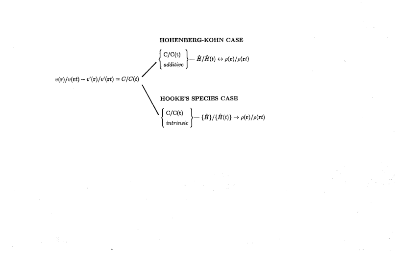
Figure 1: A schematic representation of the Hohenberg-Kohn theorem and its corollary.

The case of a set of degenerate Hamiltonians $\{{\hat{H}}\}/\{{\hat{H}}(t)\}$ that differ by a constant $C$/function $C(t)$ that is intrinsic such that the Hamiltonians represent different physical systems while yet all possessing the same density $\rho({\bf r})/\rho({\bf r}t)$, was not considered by HK/RG. In such a case, the density cannot uniquely determine the Hamiltonian, and therefore cannot differentiate between the different physical systems. This case, also shown schematically in Fig.1, corresponds to the Hooke’s species. The relationship between the set of Hamiltonians $\{{\hat{H}}\}/\{{\hat{H}}(t)\}$ and the density $\rho({\bf r})/\rho({\bf r}t)$ which is not invertible is indicated by the single-headed arrow.

We conclude by noting that the Hooke’s species, in both the time-independent and time-dependent cases, does not contitute a counter example to the HK/RG theorem. The reason for this is that the proof of the HK/RG theorem is independent of whether the constant $C$/ function $C(t)$ is additive or intrinsic. The Hamiltonians in either case still differ by a constant $C$/ function $C(t)$. A counter example would be one in which Hamiltonians that differ by more than a constant $C$/ function $C(t)$ have the same density $\rho({\bf r})/\rho({\bf r}t)$.

III.1

III.1.1

References

- (1) P. Hohenberg and W.Kohn, Phys. Rev. 136B, 864(1964).
- (2) E. Runge and E. K. U. Gross, Phys. Rev. Lett. 52, 997(1984).
- (3) T. Kato, Comm. Pure. Appl. Math 10, 151(1957).
- (4) S. Kais, D. R. Herschbach, and R. D. Levine, J. Chem. Phys. 91, 7791(1989); M. Taut, Phys. Rev. A 48, 3561(1993).
- (5) Z. Qian and V. Sahni, Phys. Rev. A. 57, 2527(1998).
- (6) S. Kais, D. R. Herschbach, N. C. Handy, C. W. Murray, and G. J. Laming, J. Chem. Phys. 99, 417(1993).
- (7) J. F. Dobson, Phys. Rev. Lett. 73, 2244(1994).