Volatility in atmospheric temperature variability

Abstract

Using detrended fluctuation analysis (DFA), we study the scaling properties of the volatility time series $V_{i}=|T_{i+1}-T_{i}|$ of daily temperatures $T_{i}$ for ten chosen sites around the globe. We find that the volatility is long range power-law correlated with an exponent $\gamma$ close to 0.8 for all sites considered here. We use this result to test the scaling performance of several state-of-the art global climate models and find that the models do not reproduce the observed scaling behavior.

, ,

1. Introduction

Indications of weather persistence over months and seasons are known [1]. This long term persistence in the atmospheric temperature variability is analysed and quantified by detrended fluctuation analysis (DFA) and wavelet transform techniques with a fluctuation exponent of $\alpha\sim 0.65$, which is independent of the location of the site [2]. Also, indications of persistence are confirmed through power spectral analysis [3, 4]. Presence of such a universal persistence law indicates that the processes governing the atmospheric dynamics at different climatological zones are based on similar principles [2]. Here, we are not interested in the temperature fluctuations around the seasonal trend, but in the magnitude of temperature changes between successive days, i.e the temperature volatility. Volatility is the concept often used in econophysics to indicate the fluctuations in price changes [5]. The market is said to be more volatile if the fluctuations in price changes are high [6]. In recent years this concept has been applied to cardiac system and found that cardiac volatility series is long range correlated [7].

Here we study the volatility of atmospheric temperature data obtained from 10 randomly chosen meteorological stations in Europe, North America, Asia, Russia and Australia, from various climatological zones. Correlations in the volatility series give information about persistence in the changes. If, for example, the change in the temperature between two successive days is small there is a high tendency that the change remains similar for the next consecutive days. Here, we study long-term temperature records (typically 100 years). We use detrended fluctuation analysis (DFA) up to the order of five [8, 9, 10], which systematically eliminates higher order trends and reveals the correlations present in the highly non-stationary data. Our analysis shows that (i) the persistence, characterised by the correlation $C(s)$ of the volatility series separated by $s$ days, follows a power law, $C(s)\sim s^{-\gamma}$, with roughly the same exponent $\gamma\cong 0.8$ for all stations considered, and that (ii) the range of this universal persistence law seems exceed one decade.

2. Methodology of Scaling analysis

We have performed the scaling analysis of volatility series for the records of the maximum daily temperature $T_{i}$ of the following weather stations: Prague (218 yr), Melbourne (136 yr), Luling (90 yr), Seoul (86 yr), Kasan (96 yr), Vancouver (93 yr), Tashkent (97 yr), New York city (116 yr), Brookings (99 yr) and St. Petersburg (111 yr). The numbers within (.) are the length of the records. From the daily maximum temperature series, we construct the volatility series $V_{i}$=$|T_{i+1}-T_{i}|$. Then we remove the climatological annual cycle [11] from $V_{i}$ to obtain $\Delta V_{i}=V_{i}-<V_{i}>$.

Qualitatively, persistence is clearly seen (patches of high and low volatility) in the plot of $V_{i}$ as shown in Fig. 1a for one year in Prague. Figure 1b shows the volatility series $\Delta V_{i}$ around the mean. Figures 1e and 1f show the plot of $V_{i}$ and $\Delta V_{i}$ respectively, obtained from the phase randomised surrogate data (preserving the distribution) [12] of the temperature increment series $(T_{i+1}-T_{i})$. Quantitatively, persistence in $\Delta V_{i}$ can be characterised by the (auto)correlation function,

$$C(s)\equiv\langle\Delta V_{i}~{}\Delta V_{i+s}\rangle=\frac{1}{N-s}\sum\limits_{i=1}^{N-s}\Delta V_{i}~{}\Delta V_{i+s},$$

where $N$ is the number of days in the record. A direct calculation of $C(s)$ is hindered by the level of noise present in finite temperature series, and by possible nonstationarities in the data. Following [13, 14], we do not calculate $C(s)$ directly, rather we study the fluctuations in the volatility profile $Y_{n}=\sum_{i=1}^{n}\Delta V_{i}$. We divide the profile into non overlapping time windows of length $s$ and determine the squared fluctuations of the profile (as specified below) in each segment. The mean square fluctuations, averaged over all segments of length $s$, are related to the correlation function $C(s)$ (see below). For this study we employ a hierarchy of methods that differ in the way the fluctuations are measured and possible nonstationarities are eliminated (see e.g.,[10, 15] for detailed description of the methods):

(i) In the simple fluctuation analysis (FA), we calculate the difference of the profile at both ends of each segment. The square of this difference represents the square of the fluctuations in each segment.

(ii) In the first order detrended fluctuation analysis, we determine in each segment the best linear fit of the profile. The variance of the profile from this straight line represents the square of the fluctuations in each segment.

(iii) In general, in the $n$-th order DFA we determine in each segment the best $n$-th order polynomial fit of the profile. The variance of the profile from these best $n$-th order polynomials represents the square of the fluctuations in each segment.

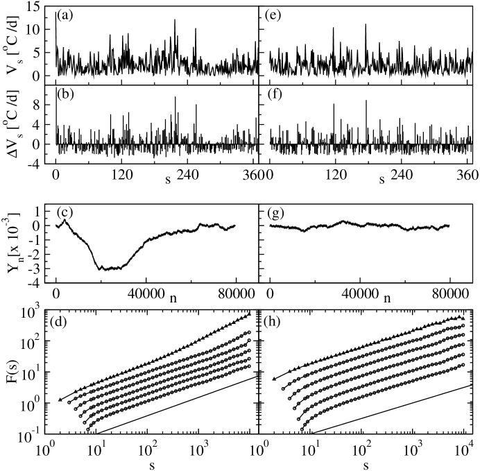
Figure 1: Temperature volatility series for Prague (1y), before removing the (climatological) annual cycle. (b) Same data as in (a) but after removing the annual cycle. (c) Profile function of the volatility series. (d) Fluctuation functions $F(s)$ obtained from the profile function shown in (c). Curves from top to bottom represent $F(s)$ obtained from FA ($\triangle$) and DFA1-5 (o). Panels (e)-(h) represent the same quantities as in (a)-(d) for phase randomised surrogate data (preserving the distribution) of the temperature increment series $(T_{i+1}-T_{i})$. Solid lines at the bottom of the panels (d) and (h) are lines with slopes 0.6 and 0.5 respectively. The unit of temperature volatility $V_{i}$ and its mean $\Delta V_{i}$ is ^∘C/$d$. Scale of $F(s)$ shown in (d) and (h) are arbitrary and the unit of $s$, $n$ and $d$ is a day.

The fluctuation function $F(s)$ is the root mean square of the fluctuations in all segments. For the relevant case of long-term power-law correlations, $C(s)\sim s^{-\gamma}$, with $0<\gamma<1$, the fluctuation function increases with $s$ according to a power law [16],

$$F(s)\sim s^{\alpha},~{}~{}~{}~{}~{}\alpha=1-\frac{\gamma}{2}.$$

For uncorrelated as well as short range correlated data, we have $\alpha=\frac{1}{2}$. For long range correlated data we have $\alpha>\frac{1}{2}$.

By definition, FA does not eliminate trends similar to the Hurst method and the conventional power spectral methods [17]. In contrast, DFAn eliminates trends of order $n$ in the profile and $n-1$ in the original time series. Thus, from the comparison of fluctuation functions $F(s)$ obtained from different methods one can learn about long term correlations and types of trends, which cannot be achieved by the conventional techniques.

Figure 2: Fluctuation functions $F(s)$ obtained from temperature volatility series for four different continental sites: Tashkent (Asia), Melbourne (Australia), New York (US) and Luling (US). Top two curves in each panel represent the $F(s)$ obtained from FA ($\blacktriangle$) and DFA2 ($\bullet$) of the volatility series. The third and fourth curves in each panel represent the $F(s)$ obtained from FA ($\triangle$) and DFA2 (o) of volatility series derived from the surrogate data. Scale of $F(s)$ is arbitrary and the unit of s is a day. Solid lines shown at the top of each panel is the line with slope 0.1 for comparison. Note that we plot $F(s)/s^{0.5}$ so that a slope of 0.1 corresponds to 0.6.

3. Scaling analysis of Temperature volatility series

We begin the analysis with the volatility series $\Delta V_{i}$ for Prague which is the longest series (218 yr) in this study. Figure 1c shows the profile, and Fig. 1d shows the fluctuation functions obtained from FA ($\triangle$) and DFA1-5 (o). In the log-log plot, all curves are approximately straight lines with a slope of $\alpha$ close to 0.6. This result suggests that there exists a long term persistence expressed by the power law decay of correlation exponent $\gamma\cong 0.8$. There is slight upward bend in the $F(s)$ curve obtained from FA. This shows that there is a trend in the volatility series, as observed in [2] for the temperature data. Hence, the effect of the city growth in Prague does not lead only to an increase in the mean temperature of the city, but also to an increase in the temperature volatility. This trend is not removed in FA while DFA1 and subsequently higher orders of DFA have removed it. Figure 1g shows the profile of the volatility series obtained from the surrogate data of the temperature increment series. When compared with Fig. 1c, profile shows much less fluctuations. Figure 1h shows the fluctuation functions $F(s)$ obtained from FA ($\triangle$) and DFA1-5 (o) for the profile shown in Fig. 1g. In the log-log plot, the fluctuation functions $F(s)$ are straight lines with a slope of $\alpha\sim\frac{1}{2}$. This shows that the original data have nonlinear features [18, 19].

Figures 2(a-d) show the results of volatility analysis for four different continental sites: Tashkent from Asia (97 yr), New York city (116 yr), Melbourne (136 yr) and Luling from Texas (90 yr). The top two curves in each panel are the fluctuation curves obtained from FA ($\blacktriangle$) and DFA 2 ($\bullet$) for volatility series of temperature data while the third and fourth curves are those obtained from the same analyses (FA and DFA2) of volatility series derived from the surrogate data. For the sake of clarity, we have divided the fluctuation function $F(s)$ by $s^{0.5}$. The straight line shown in each panel has a slope 0.1. The scaled fluctuation functions $F(s)/s^{0.5}$ obtained from the original series $\Delta V_{i}$ (the first and second curves in all panels shown in Fig. 2) are almost parallel to the line with slope 0.1. The fluctuation functions $F(s)/s^{0.5}$ obtained from the surrogate data (third and fourth curves in all panels shown in Fig. 2) are all parallel to x-axis.

We obtained similar results with exponents between 0.58 and 0.63 for all 10 sites analysed. Thus, there exist a quite general persistence law in the volatility series obtained from temperature data. The existence of such a general persistence law in the temperature volatility series indicates that the change in the temperature in different climatic zones may be governed by the same basic principles, leading to similar fluctuations in volatility series in different places.

4 Testing the volatility scaling performance of simulated temperature records

We use this result to test the state-of-the art global climate models. In an earlier work, Govindan et al.[20], have shown that temperature data simulated by GCMs violate the observed scaling behavior [2]. Here we consider the scaling analysis of the temperature volatility time series. We concentrate on four models, for which data for all three scenarios viz. Control run (CR), (ii) greenhouse gas forcing only (GHGF) and (iii) greenhouse gas plus aerosol forcing (GHGPS), are available for the same simulation period. The GCMs are: (i) CSIRO-Mk2 (Melbourne), (ii) ECHAM4/OPYC3 (Hamburg), (iii) CGCM1(Victoria, Canada) and (iv) CCSR/NIES (Tokyo) (see [21] for details).

In CR, the CO₂ content is fixed. In GHGF scenario, one mainly considers the effect of greenhouse gases. The amount of greenhouse gas forcing is taken from the historic data until 1990 and then increased at a rate of 1% per year. In GHGPS scenario, the effect of aerosols (mainly sulphates) in the atmosphere is taken into account which can mitigate and partially offset the greenhouse warming. Although this scenario represents an important step towards comprehensive climate simulation, the precise role of aerosols in the mechanism of climate modelling is still unclear.

The temperature data simulated by these four models for three different scenarios are available from the IPCC Data Distribution Center [21]. We extracted data for nine representative sites around the globe (Prague, Melbourne, Seoul, Vancouver, Kasan, Luling, Tashkent, New York and St. Petersburg). For each model and each scenario, we selected the temperature records of the four grid points closest to each site, and bilinearly interpolated the data to the location of the site.

We generate volatility series from the monthly temperature series by the same procedure (explained earlier) for daily temperature data. We removed the seasonal periodic trends in $T_{i}$ (before constructing the increment series) and also in the volatility series $V_{i}$. Since the GCMs simulate temperature data in monthly time scales, for comparison, we averaged the daily temperature (observed) data (of the nine climatological stations) to monthly data. We present our results of scaling analysis of volatility series obtained from temperature data simulated by models, for three different scenarios and also for the observed data in the form of histograms e.g. Fig. 3.

The scaling exponents $\alpha$ obtained for the observed data are shown in the topmost panel (for comparison they are plotted repeatedly for three times corresponding to three different scenarios). We can see immediately that all sites occupy the bin corresponding to the $\alpha$ value in the range of 0.58 to 0.62 (see Fig. 3 top panels) indicating the universal behavior as found in the daily data. The grey color boxes represent the $\alpha$ values of the volatility series derived from surrogate series. For the case of monthly data the $\alpha$ values obtained from the volatility series of surrogate data exhibit correlated behavior for some of the sites. However, they are well below the values of the original data. When we compare the results obtained from GCMs, none of the models show a unique behavior as found in the observed data. The $\alpha$ values are distributed widely for all the models. The comparison of the exponents of volatility series obtained from original data and that of surrogate data shows their difference is close to zero and even zero for some of the sites. For instance, in CSIRO model, for each of the three different scenarios the exponent values of the volatility series of the original data and that derived from surrogate series, have same value for St. Petersburg(9). Likewise, in ECHAM4, similar conclusion can be drawn for Kasan(5) as well as Luling(6). However, the distribution of $\alpha$ values of volatility series obtained from surrogate data, towards higher values is clearly seen for the well established scenarios like GHGF and GHGPS.

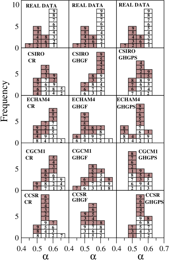
Figure 3: Histogram of DFA exponent $\alpha$ for volatility series obtained from monthly temperature data for nine different sites: Prague(1), Melbourne(2), Seoul(3), Vancouver(4), Kasan(5), Luling(6), Tashkent(7), New York(8) and St. Petersburg(9). Top three panels represent observed data. The other panels represent the exponents of volatility series obtained from temperature time series simulated by four different climate models (CSIRO-Mk2, ECHAM4/OPYC3, CGCM1 and CCSR) for three different scenarios, namely control run (CR), Greenhouse gas only forcing (GHGF) and Greenhouse gas plus sulphate forcing (GHGPS). Open boxes represent the exponents obtained for volatility series of original data while grey boxes represent the exponents obtained for volatility series derived from surrogate data of the corresponding temperature increment series.

It follows from our analysis that there is a universal persistence in the volatility series obtained from temperature increment series with an exponent of $0.60\pm 0.03$. When we use this result to test the scaling performance of the virtual climate records simulated by GCMs, we find that (i) models data display wide range of exponent values, (ii) surrogate analysis suggests that models data lack nonlinearity, especially for the well established scenarios, for some of the sites considered here.

References

- [1] J. Shukla, Science 282 (1998) 728.
- [2] E. Koscielny-Bunde, A. Bunde, S. Havlin, Y. Goldreich, Physica A 231 (1996) 393; E. Koscielny-Bunde, A. Bunde, S. Havlin, H.E. Roman, Y. Goldreich, H.J. Schellnhuber, Phys. Rev. Lett. 81 (1998) 729.
- [3] J.D. Pelletier, D.L. Turcotte, J. Hydrol. 203 (1997) 198.
- [4] P. Talkner, R.O. Weber, Phys. Rev. E 62 (2000) 150.
- [5] R.N. Mantegna, H.E. Stanley, An introduction to Econophysics (Cambridge University Press, Cambridge, 2000); P. Gopikrishnan, V. Plerou, X. Gabaix, L.A.N. Amaral, H.E. Stanley, Physica A 299 (2001) 137.
- [6] Y. Liu, P. Gopikrishnan, P. Cizeau, M. Meyer, C.-K. Peng, H.E. Stanley, Phys. Rev. E 60 (1999) 1390.
- [7] Y. Ashkenazy, P.C. Ivanov, S. Havlin, C.-K. Peng, A.L. Goldberger, H.E. Stanley, Phys. Rev. Lett. 86 (2001) 1900.
- [8] C.-K. Peng, S.V. Buldyrev, S. Havlin, M. Simons, H.E. Stanley, A.L. Goldberger, Phys. Rev. E 49 (1994) 1685;S.V. Buldyrev, A.L. Goldberger, S. Havlin, R.N. Mantegna, M.E. Matsa, C.-K. Peng, M. Simons, H.E. Stanley, Phys. Rev. E 51 (1995) 5084.
- [9] A. Bunde, S. Havlin, J.W. Kantelhardt, T. Penzel, J.H. Peter, K. Voigt, Phys. Rev. Lett. 85 (2000) 3736.
- [10] J.W. Kantelhardt, E. Koscielny-Bunde, H.H.A. Rego, S. Havlin, A. Bunde, Physica A 295 (2001) 441.
- [11] To eliminate climatological annual cycle from a series , we calculate the departures of , , from the mean values of for each calendar day , say 1 January, which has been obtained by averaging over all years in the series.
- [12] T. Schreiber, A. Schmitz, Phys. Rev. Lett. 77 (1996) 635.
- [13] M.F. Shlesinger, B.J. West, J. Klafter, Phys. Rev. Lett. 58 (1987) 1100.
- [14] H. E. Stanley, L.A.N. Amaral, J.S. Andrade, S.V. Buldyrev, S. Havlin, H.A. Makse, C.-K. Peng, B. Suki, G. Viswanathan, Phil. Mag. B 77 (1998) 1373.
- [15] R.B. Govindan, D. Vjushin, A. Bunde, S. Brenner, S. Havlin, H.J. Schellnhuber, Physica A 294 (2001) 239.
- [16] Fractals in Science, edited by A. Bunde, S. Havlin (Springer, New York, 1995).
- [17] J. Feder, Fractals, (Plenum Press, New York, 1989).
- [18] Following [19], we define a monofractal signal as a linear signal and a multifractal signal as a nonlinear signal. Volatility analysis (scaling analysis of the magnitude series) of a monofractal signal with values between will yield an uncorrelated behavior. Volatility analysis of the surrogate data of a monofractal signal will yield uncorrelated behavior. In contrary, volatility analysis of a multifractal signal will yield correlated behavior. Further, the volatility analysis of the surrogate data of the multifractal signal will yield uncorrelated behavior. Thus, for a multifractal signal, there exists a significance of difference between the volatility exponents of the data and its (volatility series derived from) surrogates.
- [19] Y. Ashkenazy, S. Havlin, P. Ch. Ivanov, C.-K. Peng, V. Schulte-Frohlinde, H.E. Stanley, preprint (cond-mat/0111396).
- [20] R.B. Govindan, D. Vjushin, A. Bunde, S. Brenner, S. Havlin, H.J. Schellnhuber, Phys. Rev. Lett. 89 (2002) art. no. 028501.
- [21] http://ipcc-ddc.cru.uea.ac.uk/dkrz/dkrz_index.html