Late stages of coarsening in model C

Abstract

We present a comprehensive picture of (non-critical) domain growth in model C systems where a non-conserved scalar order parameter is coupled to a conserved concentration field. For quenches into the region where the ordered and disordered phases coexist, we confirm earlier partial numerical results and find a growth exponent $z=3$. For quenches into the ordered region, we confirm the theoretical prediction $z=2$. Finally we discuss the implications of our results for domain growth in the microcanonical $\phi^{4}$-model and we offer some criticism of the work of Somoza and Sagui on the morphology and wetting properties of domains.

I Introduction

Coarsening has been a object of intensive study over the last decades not only because of its experimental relevance but also because it constitutes what is maybe the simplest case of out-of-equilibrium dynamics. For a scalar order parameter, one generally distinguishes the non-conserved case, e.g. the Ising model with Glauber dynamics (model A according to the widely-used classification of [1]), from the conserved case, e.g. the Ising model with Kawasaki dynamics (model B). It is now well-established that in these cases phase ordering is characterized by a single lengthscale $L$ growing algebraically with time ($L\sim t^{1/z}$) with the growth exponent $z$ taking two different values, $z=2$ for the non-conserved/model A case, and $z=3$ for conserved order parameter systems like model B [2]. Here we are interested in the more complicated and therefore less well understood case of a non-conserved order parameter coupled to a conserved concentration (so-called model C). Examples of this situation can be found in various physical systems, e.g., intermetallic alloys (see [3] and references therein), adsorbed layers on solid substrates [4] and supercooled liquids [5]. In these systems, the decomposition process (described by the conserved concentration $c$) and the ordering process (described by the non-conserved order parameter $\psi$) are coupled. Let us consider an $A-B$ alloy on a square lattice in order to illustrate this. A state in which all $A$ atoms are surrounded by $B$ atoms is energetically favorable. The ordered state thus consists of two symmetric sublattices, and we can define an order parameter $\psi$ as half of the difference between the $A$-concentration in each sublattice. In this way, $\psi=1$ when all the $A$ atoms are on the one sublattice and $\psi=-1$ when they are on the other. At high temperature, a disordered state $\psi=0$ arises. It is now easy to realize that for asymmetric initial conditions (i.e. an unequal amount of $A$ and $B$ atoms) the system will not be able to completely order (strictly speaking, this is only true at low-enough temperature). Hence, as opposed to model A, the disordered phase can coexist with the two ordered phases. On a typical equilibrium phase diagram in the concentration-temperature ($c$-$T$) plane (Fig. 1), one can thus distinguish, apart from a disordered region and an ordered region, a coexistence region. The dashed line separating the ordered and disordered regions marks a second-order phase transition. In the spinodal region inside the coexistence region (dotted line), the three phases are thermodynamically unstable.

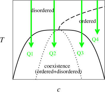
FIG. 1.: Typical equilibrium phase-diagram of a model C in the ($c,T$) plane. The solid line is the coexistence curve, the dashed curve is the order-disorder transition line. The dotted line within the coexistence region is the spinodal curve inside which the three phases are unstable. Four different types of quenches (Q1, Q2, Q3, and Q4) are shown.

Models have been proposed to account for various aspects of the morphology and of the kinetics of the experimental systems (see for instance [3] and references therein). From the more theoretical point of view of universality issues, the situation is not quite satisfactory. For instance, the critical exponents, and in particular the dynamic critical exponent, are still debated [6, 7, 8]. A renormalization group analysis turns out to be more delicate than in the case of model A [9, 10]. Our goal here is to clarify the a priori simpler problem of domain growth below criticality, when the system is quenched down from a high-temperature state. Notable but partial results, somewhat scattered in the literature, have been obtained in the past. For quenches into the spinodal region with droplet morphology (quench Q2 of Fig. 1) San Miguel et al. [11] have predicted the model B exponent $z=3$. Numerical simulations in the context of a Oono-Puri “cell model” have been found to be consistent with this prediction[12, 13]. On the other hand, Elder et al. [14] have predicted $z=2$ for quenches above the tricritical temperature, i.e. in the ordered region (quench Q4). To the best of our knowledge, this has not been verified numerically.

Our goal here is to give a complete picture of (non-critical) domain growth in model C, considering, within a single system introduced in Section II, all four possible types of quenches illustrated in Fig. 1. This is done in Section III. In Section IV, in the sake of comprehensiveness, we come back to the two following unsettled issues discussed recently in works about model C systems. The microcanonical $\phi^{4}$ model [15, 16, 7], is a type of model C since the order parameter is coupled to the (conserved) energy. Zheng has suggested in a recent paper [17] that domain growth is characterized by a non-trivial value of $z$ ($2<z\simeq 2.65<3$). A more careful study by us showed that the data are in fact consistent with the model A exponent $z=2$ [18]. Here we detail to which phase of model C the microcanonical $\phi^{4}$ model belongs. The morphology of domains and the related “wetting” issues have also been a point of contention in the past. In experiments, it has been observed that neighboring ordered domains do not merge [19]. A possible explanation proposed in [20] is that the domains are different variants of the same ordered structure. The simulations of [3] seem to indicate that ordered domains do not join but “stay separated by narrow channels of the disordered phase”: the antiphase boundaries appear to be wetted by the disorder phase. But Somoza and Sagui [22] have found on the contrary that inside the coexistence region the two ordered phases may be in direct contact. We revisit their work and resolve the controversy. A summary of our results is given in Section V.

II The model

We choose one of the simplest versions of model C which can be written as follows:

$$\frac{\partial\psi}{\partial t} = -\Gamma_{\psi}\frac{\delta F}{\delta\psi}+\eta$$ (1)

$$\frac{\partial c}{\partial t} = \Gamma_{c}\nabla^{2}\frac{\delta F}{\delta c}+\eta^{\prime}.$$ (2)

Here $\Gamma_{\psi}$ and $\Gamma_{c}$ are kinetic coefficients, $\eta$ and $\eta^{\prime}$ represent thermal noise and $F[\psi,c]$ is the Ginzburg-Landau free energy functional which takes generally the following form:

$$F[\psi,c]=\!\int\!d^{n}r\left[f(c,\psi)+\frac{K_{c}}{2}(\nabla c)^{2}+\frac{K_{\psi}}{2}(\nabla\psi)^{2}\right],$$ (3)

where $K_{c}$ and $K_{\psi}$ are diffusion constants. The function $f(c,\psi)$ should satisfy a few constraints. Firstly it has to be symmetric in $\psi$: $f(c,\psi)=f(c,-\psi)$. It should also allow for the coexistence of a disordered phase $(c_{n},\psi_{n})$ with the ordered phases $(c_{s},\pm\psi_{s})$ [21]. These points correspond to minima in the free energy landscape. A possible choice is [22, 23]

$$f(c,\psi)=\psi^{2}(1-\psi^{2})^{2}+\alpha(\psi^{2}-c)^{2}\;,$$ (4)

where $\alpha$ governs the coupling between the two fields. The minima are then $(c_{n},\psi_{n})=(0,0)$ corresponding to the disordered phase and $(c_{s},\psi_{s})=(1,\pm 1)$ corresponding to the ordered phase.

It is instructive to analyze the model in terms of its uniform fixed points $(c_{0},\psi_{0})$. They lie on the curves where $f_{\psi}=0$ which are the $c$-axis $\psi_{0}=0$ and the polynomial $c_{0}=\frac{1}{4\alpha}(1-3\psi_{0}^{2})(1-\psi_{0}^{2})+\psi_{0}^{2}$. Their stability is determined by the signs of $f_{\psi\psi}$ and $(f_{cc}f_{\psi\psi}-f_{c\psi}^{2})$ [11, 23].

Fixed points on the $c$-axis change stability at the so-called ordering spinodal $c_{1}$: they are stable for $c<c_{1}=\frac{1}{4\alpha}$. The point on the second curve where stability changes is the conditional spinodal $c_{\sigma}$. Stability occurs when $c>c_{\sigma}=\frac{4\alpha-1}{6\alpha}$.

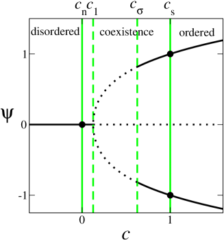
FIG. 2.: ($c$,$\psi$)-plane. Solid lines: stable uniform fixed points. Dotted lines: unstable uniform fixed points. The minima of $f$ are indicated by filled circles. Grey lines delimit the coexistence domain. Dashed grey lines delimit the spinoidal region

Consider now the evolution of a two-dimensional system starting from random initial conditions disordered around $\psi=0$ with some fixed concentration $c_{i}$. We briefly present the expected follow-up of quenches at various $c_{i}$ values before describing our corresponding numerical results in the next section.

— For $c_{i}<c_{n}$ (disordered phase), the system evolves towards the stable point $(c_{i},0)$.

— For $c_{n}<c_{i}<c_{s}$, the three phases $(0,0)$ and $(1,\pm 1)$ can in principle coexist.

— For $c_{n}<c_{i}<c_{1}$ (quench Q1), however, $(c_{i},0)$ is still stable and it will be reached if initial fluctuations are small enough.

— Inside the region $c_{1}<c_{i}<c_{\sigma}$ (quench Q2), the system necessarily undergoes spinodal decomposition. For $c_{\sigma}<c_{i}<c_{s}$ (quench Q3), even though the ordered fixed points are now stable, nothing is changed since the initial conditions (chosen around $\psi=0$) lead to the formation of disordered domains.

— For initial concentrations $c_{i}>c$ (quench Q4), the system will not phase separate but will order, so we identify this region with the ordering regime.

III Numerical results

In order to investigate the late stages of domain growth, Eqs. (1-2) are now studied numerically. We perform quenches from the high-temperature disordered phase to $T=0$. (The noise term in Eqs. (1-2) can be set equal to zero, since the growth exponent is expected to be determined by the “$T=0$ fixed point” [2].) In practice, initial conditions are randomly distributed around $(c_{i},0)$. More specifically, we choose $\psi\in[-0.1:0.1]$ and $c\in[c_{i}-0.05:c_{i}+0.05]$.

Equations (1-2) are numerically solved on a two-dimensional grid. For the time integration we use Euler’s method and we approximate the Laplacian by:

$$\nabla^{2}y=\frac{1}{\Delta x^{2}}\left[\frac{1}{6}\sum_{{\bf j}\in{\cal V}_{i}^{1}}y_{\bf j}+\frac{1}{12}\sum_{{\bf j}\in{\cal V}_{i}^{2}}y_{\bf j}-y_{\bf i}\right]$$ (5)

where ${\cal V}_{i}^{1}$ and ${\cal V}_{i}^{2}$ are the sets of nearest and next-nearest neighbors of site $i$.

In most regimes studied below, $\Delta x=1.0$ and $\Delta t=0.01$ allow for a smooth representation of both fields. Without loss of generality, we set: $K_{c}=K_{\psi}=1$ and $\alpha=4$. We record the typical domain size $L$ of both the order parameter and the concentration fields, as determined by the mid-height value of $C_{c,\psi}(r,t)$, the normalized two-point correlation function calculated for simplicity along the principal axes of the lattice using the the reduced “spin” variables $\sigma_{\psi}\equiv{\rm sign}(\psi)$ and $\sigma_{c}\equiv{\rm sign}(c-c_{i})$:

$$C(r,t)=\langle\frac{1}{2}(\sigma_{i+r\,j}(t)+\sigma_{i\,j+r})\sigma_{ij})\rangle-\langle\sigma_{ij}\rangle^{2}$$ (6)

A Quenches into the coexistence regime: droplet regime

Quenches within the disordered regime being uninteresting, we first discuss Q1 quenches, i.e. quenches into the coexistence region, but left of the spinodal ($c_{n}<c<c_{1}$). Here the system possesses a stable fixed point $(c_{i},0)$ but will be able to locally reach the ordered fixed points if initial fluctuations are large enough. The precise dependence on initial conditions is in fact a non-trivial problem that we have not studied systematically. This shows that the spinodal lines do not have a strict meaning in the presence of fluctuations, a well-known fact (see for instance [24]).

When decomposition occurs, the ordered phase is the minority phase, and, similarly to what is observed in model B, droplets of either ordered phases form. A similar configuration is shown in Fig. 4. The growth of ordered droplets is constrained by the conservation law. The smallest droplet disintegrates to the benefit of the larger ones. We thus expect a Lifshitz-Slyozov growth law $L\sim t^{1/3}$. In our simulations, this behavior is not easily observed, due to the presence of a long transient during which the ordered domains “nucleate” out of the metastable state. In particular, the growth of the typical lengthscales $L_{c,\psi}$ does not show the expected scaling although the trend at large times is good. In this regime, though, the droplet morphology of the ordred domains can be exploited to provide a more direct measurement of growth. In Fig. 3, we show the evolution of the total number of the ordered droplet,s $n$, and of the average droplet volume $V$. These quantities scale respectively as $t^{-2/3}$ and $t^{2/3}$. Due to a long crossover, the expected behavior is only clearly seen when plotting $V$ and $1/n$ against $t^{2/3}$ (Fig.3b).

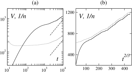
FIG. 3.: Domain growth at $c_{i}=0.1$. (a) $V$ and $1/n$ (dotted lines) vs. $t$ in log-log plot. The dashed lines indicate the expected asymptotic behavior $V$,$1/n~{}t^{2/3}$ (b) $V$ and $1/n$ vs. $t^{2/3}$ ($1/n$ is multiplied with some factor so that it can diplayed together with $V$). System size is $2048\times 2048$.

The same scenario is observed for Q2 quenches provided the ordered phase be the minority phase, i.e. for $c_{1}<c_{i}<\frac{c_{n}+c_{s}}{2}=0.5$. A typical snapshot is shown in Fig. 3. We have also verified that indeed a growth exponent $z=3$ is observed. Now the crossover is shorter and we see that the local slope of $\log L_{c,\psi}$ vs $\log t$ approaches $\frac{1}{3}$ at late times (see Fig. 5ab). The same conclusion is reached studying the total number of domains and their average volume (Fig. 5cd).

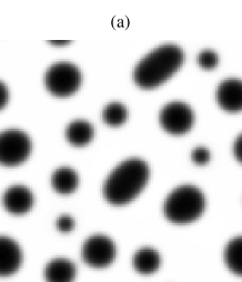
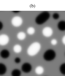
FIG. 4.: Snapshots of coarsening in droplet regime ($c_{i}=0.25$) for a system of $128\times 128$ at $t=200$. High values of the field correspond to dark areas. (a) concentration field: white corresponds to the disordered phase $c=0$, black to the ordered phase $c=1$, (b) order parameter field: grey corresponds to the ordered phases $\psi=0$, white and black correspond to the ordered phases $\psi=\pm 1$.

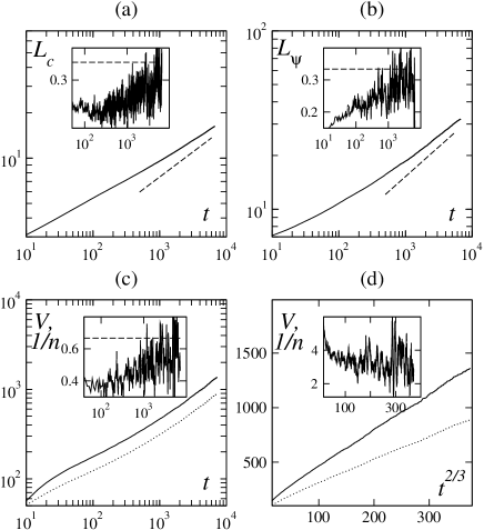
FIG. 5.: Domain growth in the droplet regime ($c_{i}=0.25$) (a) $L_{c}$ vs $t$ (b) $L_{\psi}$ vs $t$ (c) $V$ and $1/n$ (dotted lines) vs $t$ (d) $V$ and $1/n$ vs $t^{2/3}$. (a),(b) and (c) are on logarithmic scale, (d) is in linear scale. The dashed lines indicate the expected scaling / exponent values. Insets: local slopes calculated by a running average of the derivated signal over a window of fixed size in the corresponding variable (i.e. $\log_{10}t$ or $t^{2/3}$ here). System size is $4096\times 4096$.

B Quenches into the coexistence regime: interconnected regime

Due to the coupling to the non-conserved order parameter, the symmetry between high and low concentration phases, which exists in model B, is broken. For $c_{i}>1/2$ the minority phase (now the low concentration phase) does not form droplets but is instead concentrated along lines which correspond to interfaces of the non-conserved field. In the context of alloys one speaks of “wetting of antiphase boundaries”. Looking at the non-conserved field, we first observe model A like coarsening which then slows down, since the interfacial regions separating ordered domains get wider (made of the disordered phase, their volume is conserved). We thus again encounter the situation where the ordering is constrained by the conservation law, but with the difference that the disordered phase has a particular morphology. It is therefore not obvious that the growth exponent will be $z=3$. The derivation of [11] is only valid in the case of isolated droplets. However, the Lifshitz-Slyozov law is known to apply more generally, provided that 1) coarsening is driven by surface tension, 2) transport is by diffusion through the bulk and 3) the length scale that describes the coarsening process is the only relevant length scale in the system [25]. It is easy to convince oneself that the first two conditions are fulfilled. At first sight, however, it appears that there are two lengthscales: one associated with the thickness of the disordered domains, $d$ (equivalently of the interfaces between ordered domains), the other with their curvature (equivalent to the lengthscale of the ordered domains), $L$. One has to realize that the total interface length $l$ is inversely proportional to $L$. Since the volume occupied by the interface is conserved we also have $d\sim 1/l$, and therefore $d\sim L$. One thus expects again a growth exponent $z=3$.

The above discussion not only applies to Q2 quenches ($1/2<c_{i}<c_{\sigma}$), but also to Q3 quenches ($c_{\sigma}<c_{i}<c_{s}$). A uniform configuration $(c_{0},\psi_{0})$ is then stable, but for symmetric initial conditions there are always interfaces where $\psi=0$ and where it is thus more favorable to have $c<c_{i}$. In the “ordered” domains $c$ will then increase such that we will end up with all the three phases.

All this is confirmed by our numerical results. In Fig. 6 we show snapshots of order parameter and concentration at late times for $c_{i}=0.5$ and $c_{i}=0.75$. In Fig. 7 we plot, for the same concentrations, the typical lengthscale of ordered domains and disordered domains. They behave similarly. We can also identify two transient effects. Initially, rapid growth takes place due to the ordering process. After that, when the antiphase bounderies are wetted, the growth will actually be slower than $L\sim t^{1/3}$. Since the disordered phase has a large surface compared to its volume, surface diffusion will dominate at short times, and this is known to lead to a $L\sim t^{1/4}$ growth law [26].

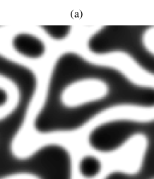
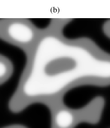
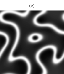
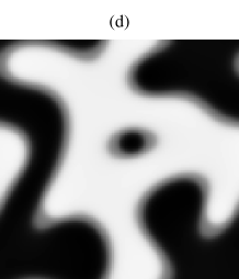
FIG. 6.: Snapshots of coarsening in interconnected regime (a) Concentration field and (b) order parameter field at $c=0.5$ at $t=200$ (c), (d) id. at $c=0.75$ at $t=120$ System size and greyscales as in Fig. 4.

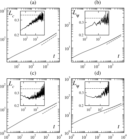
FIG. 7.: Domain growth in interconnected regime (a) $L_{c}$ vs $t$ ,(b) $L_{\psi}$ vs $t$ both at $c=0.5$, (c) $L_{c}$ vs $t$ ,(d) $L_{\psi}$ vs $t$ both at $c=0.75$ The local slopes in the insets are calculated as explained in Fig. 5. System size $4096\times 4096$.

C Ordered regime

For $c_{i}\geq c_{s}=1$ (Q4 quenches) no spinodal decomposition occurs. If initially a domain of the disordered phase exists, it disappears. Although the concentration is not completely uniform but somewhat lower at the interfaces of the ordered domains, as seen in Fig. 9, this does not have any influence on the coarsening of the order parameter. Thus, the model A exponent $z=2$ should be observed for $c_{i}\geq 1$. Again this is confirmed in our simulations. We have measured the typical domain size for the order parameter around $c_{s}$. As can be seen in Fig. 9 a growth exponent $z=3$ is still observed for $c_{i}$ slightly below $c_{s}$, at $c_{i}=0.95$. At $c_{i}=c_{s}$, growth is clearly faster but the local exponent (inset of Fig. 9c) does not reach $\frac{1}{2}$ in accessible times. The behavior, though, is consistent with $z=2$. This is most clearly observed plotting $L$ againt $\sqrt{t}$ (Fig. 9b). Increasing $c_{i}$ beyond $c_{s}$, the crossover is now short enough and the $z=2$-behavior is apparent even in a log-log plot (Fig. 9d).

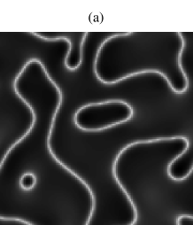
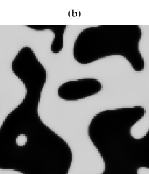
FIG. 8.: Snapshots of coarsening in ordered regime ($c_{i}=1.5$) at $t=50$ (a) concentration field (b) order parameter field. System size and greyscale as in Fig. 4.

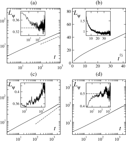
FIG. 9.: Growth of typical order parameter domain size $L_{\psi}$ (a) $c_{i}=0.95$ (b),(c) $c_{i}=1.0$ (b): $L$ vs. $t^{1/2}$ (d) $c_{i}=1.5$. The local slopes in the insets are calculated as explained in Fig. 5. The system size is $4096\times 4096$.

IV Discussion

A The microcanonical $\phi^{4}$ model

The microcanonical $\phi^{4}$ model has lately received renewed attention largely because it offers an interesting bridge between statistical mechanics and deterministic dynamics [16, 15, 7]. Its equations of motion derive from the well known lattice $\phi^{4}$ Hamiltonian. They can be written:

$$\ddot{\phi_{i}}=\sum_{j}(\phi_{j}-\phi_{i})+m^{2}\phi_{i}-\frac{g}{6}\phi_{i}^{3}$$

where the sum is over the 4 nearest neighbors of site $i$ on a square lattice.

As stated before, this model is believed to be in the model C universality class since the order parameter $\phi$ is coupled to the conserved energy. [1] Indeed, looking at snapshots of the order parameter and the local energy, defined as:

$$E_{i}=\frac{1}{2}\dot{\phi_{i}}^{2}-\frac{1}{2}m^{2}\phi_{i}^{2}+\frac{g}{4!}\phi_{i}^{4}+\sum_{j=1}^{d}(\phi_{i+j}-\phi_{i})^{2}\;,$$ (7)

one observes that $E_{i}$ is higher at the interfaces of ordered domains (Fig. 10a) as observed in our model C around the coexistence concentration $c_{s}$. Given the results described above, the question of the precise relationship between the microcanonical $\phi^{4}$ model and model C now boils down to whether we are in the interconnected ($(c_{n}+c_{s})/2<c_{i}<c_{s}$) or the ordered regime ($c_{i}>c_{s}$) of model C, i.e. whether the interfaces (equivalently the disordered domains) will thicken or not.

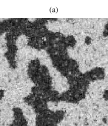
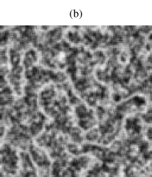
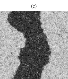
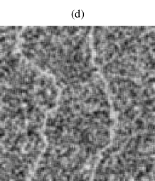
FIG. 10.: Snapshots of (a) order parameter $\phi$ and (b) energy density $E$ at time $t=15$, (c),(d): id. but at $t=75$.

Our observation that, in fact, $z=2$ [18] indicates that we are in the ordered regime. This implies that the conserved field does not undergo spinodal decomposition. The snapshots of the order parameter and the local energy taken during coarsening (Fig. 10) reveal that the width of the “antiphase boundaries” does not grow. Instead, energy flows into the bulk of domains in the form of kinetic energy, as observed in [18]. The increase of kinetic energy compensates the energy lost due to the decrease of the total interface length. We believe this constitutes further support to our result $z=2$, at least for the parameter values studied in [17] and [18]. Whether a coexistence regime in the $\phi^{4}$-model exists for other parameter values remains, strictly speaking, an open question. In fact, since the system is isolated, the total energy and the “temperature” cannot be varied independently. Upon increasing the energy, the temperature, which can be identified with the kinetic energy, will also increase. We therefore only have access to a line in the $(c,T)$-plane of Fig. 1. (Note that increasing the energy corresponds to decreasing the concentration.) Investigations of the critical behavior of the model, where it is a priori important whether one enters the disordered region from the coexistence region or from the ordered region, are under way [28].

B Interfacial properties

A few years ago, Somoza and Sagui have investigated the effect of interfacial properties on the morphology of domains in a model C system [22]. They came to the conclusion that apart from a “complete wetting” regime where two “ordered” domains ($\psi=\pm 1$) are always separated by a disordered layer ($\psi=0$), there exist also a “partial wetting” and even a “partial drying” regime where ordered domains of opposite sign can be in direct contact. These regimes were observed by varying the diffusion constants $K_{c}$ and $K_{\psi}$ keeping $\Delta x$ and $\Delta t$ fixed. Thus diffusion of one quantity was enhanced with respect to the other.

We first repeated the simulations of Somoza and Sagui using $\Delta x=1$. (Fig. 11a). The ordered domains are in direct contact but the corresponding interfaces are not smooth, an indication that the equations are not well resolved. Next, we performed the same quench but at a higher numerical resolution ($\Delta x=0.3$). As shown in Fig. 11b, no direct contact between ordered domains can be observed. The argument put forward in [22] is that in the partial drying regime the surface tension is lower between the two ordered phases than between the ordered and disordered phases. This surface tension was measured by calculating the free energy of a numerically obtained interface profile [27]. It must be noted, however, that this procedure is only correct when the obtained profile is the equilibrium profile. An order-order interface for instance will desintegrate into two disorder-order interfaces when the surface tension of the latter is lower. The speed at which this happens depends on the diffusion constants, since some amount of the conserved quantity has to diffuse away from the interface. One could thus have the impression that an order-order interface is stable, when in fact it is very slowly disintegrating.

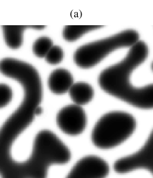
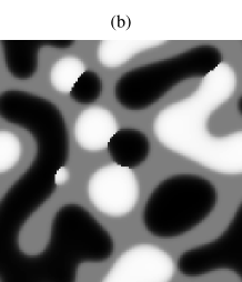
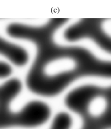
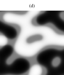
FIG. 11.: Snapshots of partial wetting regime $K_{\psi}=0.6$, $K_{\psi}=1/K_{c}$ with $\Delta x=1.0$, $\Delta t=0.01$. (a) Concentration field, (b) Order parameter (c),(d), Same system but better resolved: $\Delta=0.3$, $\Delta t=0.005$. System size and greyscales are in same as in Fig. 4.

V Conclusion

We have provided a comprehensive account of domain growth in two-dimensional model C systems, unifying and sometimes correcting partial results present in the literature. Quenches into the coexistence region ($c_{n}<c_{i}<c_{s}$) all lead to $z=3$ domain growth governed by the conserved field, independent of the morphology of domains, but subjected to the strength of initial fluctuations when $c_{i}<c_{1}$. Quenches into the ordered region are asymptotically dominated by the ordering process, leading to $z=2$ growth after a crossover from slower $z=3$ coarsening.

We also clarified the status of the microcanonical $\phi^{4}$ model and showed that in this case sub-critical domain growth correspond to quenches into the ordered region of model C.

The picture that thus emerges is that domain growth in model C systems below criticality is governed by the growth exponent of either model A or model B. At criticality, on the other hand, one may expect exponents different from model A or B. The natural question that then arises is how the exponents depend on on the initial concentration.

Another issue open for further investigation is the behavior of the so-called persistence probability $p$, defined as the probability for a spin to have remained in its initial phase from $t_{0}$ up to time $t$ (see [29] for a review). In the case of model A and B this quantity decays algebraically with an exponent $\theta$, estimated to be $\theta_{A}\approx 0.21$ [30] and $\theta_{B}\approx 0.25$ [31]. The universality of these exponents is an ongoing debate. Measurements of the persistence exponent in model C, especially in the interconnected regime where one would expect the model B value, might help to settle this issue.

REFERENCES

- [1] P.C. Hohenberg and B.I. Halperin, Rev. Mod. Phys. 49, 436 (1977).
- [2] A. J. Bray, Adv. Phys. 43, 357 (1994).
- [3] V.I. Gorentsveig, P. Fratzl, and J.L. Lebowitz, Phys. Rev. B 55, 2912 (1997).
- [4] K. Binder, W. Kinzel and D.P. Landau, Surf. Sci. 117, 232 (1982)
- [5] H. Tanaka, J. Phys.: Condens. Matter 11, L159 (1999)
- [6] D. Stauffer, Int. J. Mod. Phys. C 8, 1263 (1997); P. Sen, S. Dasgupta, and D. Stauffer, Eur. Phys. J. B 1, 107 (1998)
- [7] B. Zheng, M. Schulz, and S. Trimper, Phys. Rev. Lett. 82, 1892 (1999).
- [8] G. Besold, W. Schleier, and K. Heinz, Phys. Rev. E 48, 4102 (1993).
- [9] E. Brezin and C. De Dominicis, Phys. Rev. B 12, 4954 (1975).
- [10] K. Oerding and H.K. Janssen, J. Phys. A 26, 3369 (1993).
- [11] M. San Miguel, J.D. Gunton, G. Dee, and P. Sahni, Phys. Rev. B 23, 2334 (1981).
- [12] T. Ohta, K. Kawasaki, A. Sato, and Y. Enomota, Phys. Lett. A, 126, 93 (1987).
- [13] A. Chakrabarti, J.B. Collins, and J.D. Gunton, Phys. Rev. B 38, 6894 (1988).
- [14] K.R. Elder, B. Morin, M. Grant, and R.C. Desai, Phys. Rev. B 44, 6673 (1991).
- [15] L. Caiani, L. Casetti, C. Clementi, G. Pettini, M. Pettini, and R. Gatto, Phys. Rev. E 57, 3886 (1998); and references therein.
- [16] L. Caiani, L. Casetti, and M. Pettini, J. Phys. A 31, 3357 (1998).
- [17] B. Zheng, Phys. Rev. E 61, 153 (2000).
- [18] J. Kockelkoren and H. Chaté, Phys. Rev. E 65, 058101 (2002).
- [19] T. Miyazaki, H. Imamura, and T. Kozakai Mater. Sci. Eng. 54, 9 (1982)
- [20] Y. Wang and A. Khachaturyan, Scripta Metall. et Mat. 31, 1425 (1994).
- [21] We use the same notation as in the seminal paper by: P.C. Hohenberg and D.R. Nelson, Phys. Rev. B 20, 2665 (1981).
- [22] A.M. Somoza and C. Sagui, Phys. Rev. E 53, 5101 (1996).
- [23] H.P. Fischer and W. Dieterich, Phys. Rev. E 56, 5909 (1997).
- [24] K. Binder, Phys. Rev. A 29, 341 (1984).
- [25] J.L. Langer in Solids far from equilibrium, C. Godrèche, editor (Cambridge University Press, 1991)
- [26] D.A. Huse, Phys. Rev. B 34, 2665 (1981).
- [27] A.M. Somoza, private communication
- [28] Ph. Marcq and H. Chaté, unpublished
- [29] For a recent review, see, e.g., S.N. Majumdar, Current Science 77, 370 (1999) (also as preprint cond-mat/9907407).
- [30] S. Cueille and C. Sire, Eur. Phys. J. B 7, 111 (1999).
- [31] J. Kockelkoren and H. Chaté, Phys. Rev. E 62, 3004 (2000); J. Kockelkoren, A. Lemaître, and H. Chaté (unpublished).