Comment on “Deterministic equations of motion and phase ordering dynamics”

Abstract

Zheng [Phys. Rev. E 61, 153 (2000)] claims that phase ordering dynamics in the microcanonical $\phi^{4}$ model displays unusual scaling laws. We show here, performing more careful numerical investigations, that Zheng only observed transient dynamics mostly due to the corrections to scaling introduced by lattice effects, and that Ising-like (model A) phase ordering actually takes place at late times. Moreover, we argue that energy conservation manifests itself in different corrections to scaling.

The problem of the dynamical foundations of statistical mechanics has received renewed attention recently, when, in the spirit of the famous work of Fermi, Pasta, and Ulam [1], researchers directly studied the evolution of isolated, many-degrees-of-freedom Hamiltonian systems with the aim of relating their microscopic, deterministic, chaotic motion to their macroscopic statistical properties [2]. In this context, the two-dimensional lattice $\phi^{4}$ model is of special interest because it is known to exhibit, within the canonical ensemble, a second-order phase transition in the Ising universality class. Recent work [3, 4] aimed, in particular, at studying the corresponding behavior in the isolated, microcanonical case, whose equations of motion can be written:

$$\ddot{\phi_{i}}=\sum_{j}(\phi_{j}-\phi_{i})+m^{2}\phi_{i}-\frac{g}{6}\phi_{i}^{3}$$

where the sum is over the four nearest neighbors of site $i$ on a square lattice.

In the same spirit, Zheng [5] has considered the a priori simpler problem of the phase-ordering process which takes place when the microcanonical $\phi^{4}$ lattice is suddenly “quenched” below the critical point. Universality of domain growth laws is nowadays a fairly well-established topic [6]. It is well documented, even for less traditional systems such as deterministic, possibly chaotic, spatially-extended dynamical systems [7, 8, 9, 10]. For a scalar order parameter, two main universality classes can be distinguished depending on whether it is locally conserved or not. The Ising model is prototypical of the non-conserved case, and so should be the lattice $\phi^{4}$ model, at least in the usual canonical ensemble point of view. However, and this was the interesting point raised by Zheng, the presence of the energy conservation in the microcanonical case might have an influence on the dynamical scaling laws associated with phase ordering. In this sense, the question is whether the phase ordering of model C [11] is in the same universality class as model A.

Using numerical simulations in the so-called “early-time” regime, Zheng confirmed that the usual dynamical scaling laws seem to hold, but with exponents at odds with those both the non-conserved order parameter (NCOP) and the conserved order parameter (COP) class [5]. In particular, he found $z=2.6(1)$ ( $1/z$ is the exponent governing the algebraic growth of $L$, the typical size of domains), between its NCOP and COP values ($z_{\rm NCOP}=2$ and $z_{\rm COP}=3$). Zheng “explains” this surprising result by the influence on scaling of “the fixed point corresponding to the minimum energy of random initial states” (present when considering domain growth).

Here we show that a more careful numerical investigation actually leads to conclude that the microcanonical lattice $\phi^{4}$ model shows normal, NCOP phase-ordering. We argue that energy-conservation, but also lattice effects, have sub-leading influences on scaling. We discuss in particular the effect of the increase of the “bulk temperature” due to the progressive disappearance of interfaces during the growth transient. We attribute the erroneous results of Zheng to the danger of using “early-time” methods and naive logarithmic plots in problems with large microscopic times and/or corrections to scaling.

I Normal scaling at late times

Zheng conducted different numerical experiments which led to estimates of exponents $z$, $\lambda/z$ (where $\lambda$ is the so-called Fisher-Huse exponent), and $\theta=(2-\lambda)/z$. From all direct measurements of $z$ he concluded that $z=2.6(1)$. Using this value, he found an estimate of $\lambda$ in agreement with the NCOP value ($\lambda=1.22(5)$ whereas $\lambda_{\rm NCOP}=5/4$). Thus, the only strong departure from the NCOP values is for exponent $z$. Therefore, in the following, we focus on growth law of $L$ in large systems at late times (as opposed to the early-time approach favored by Zheng).

In order to reach late times satisfactorily, we need a better control of the conservation of energy than with the simple second-order scheme used by Zheng. The following results were obtained with a third-order bilateral symplectic algorithm [12] with a timestep $dt=0.025$. The conservation of initial energy is better than $10^{-5}$ in relative value in all runs presented. To investigate phase-ordering, we use the same initial conditions as Zheng ($\phi=\pm q_{0}$ where the sign is random and $q_{0}$ calculated to yield the desired energy density $\epsilon$). We present results for two sets of parameter values, $(m^{2},g)=(6,1.8)$ (set A, used by Zheng), and $(m^{2},g)=(2,0.6)$ (set B, used in [3, 4]). The initial energy density ($\epsilon_{0}=27$ for set A, and $\epsilon_{0}=10.0001$ for set B), was chosen very close to its minimum value allowed by the random-sign initial conditions ($\epsilon_{\rm min}=80/3$ for set A, and $\epsilon_{\rm min}=10$ for set B). This ensures that “thermal” fluctuations are minimized, since the energy density is then as far as possible from the critical energy density $\epsilon_{\rm c}$ ($\epsilon_{\rm c}\approx 35$ for set A, and $\epsilon_{\rm c}\approx 21$ for set B).

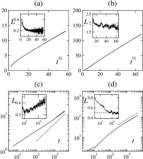
FIG. 1.: Growth of typical scale $L(t)$. All results presented here were obtained from single runs of lattices of $8192\times 8192$ sites with periodic boundary conditions. (a,b): $L$ vs $\sqrt{t}$ for parameter set A and B, the dotted lines are the fits discussed in section II C; (c,d): same but in logarithmic scales (dashed lines for “expected” behavior $z=2$). Insets: local slopes calculated by a running average of the derivated signal over a window of fixed size in the corresponding variable (i.e. $\sqrt{t}$ or $\log_{10}t$ here). For (a,b) window size $\Delta(\sqrt{t})=0.5$; For (c,d) window size $\Delta(\log_{10}{t})=0.05$.

A Growth of typical domain size

The typical domain size $L$ was determined by the mid-height value of $C(r,t)$, the normalized two-point correlation function calculated for simplicity along the principal axes of the lattice using the continuous field $\phi$ or the reduced “spin” variable $\sigma\equiv{\rm sign}(\phi)$: $C(k,t)=\frac{1}{2N}\sum_{ij}\sigma_{ij}(\sigma_{i+k\ j}+\sigma_{i\ j+k})$. (No significant difference was found between the two cases, and only results using $\sigma$ are shown below.) We first checked that dynamical scaling holds by observing the collapse of $C(r,t)=f(r/L(t))$ curves at different times after some transient (not shown) [19].

For both sets of parameters, the expected NCOP law ($L\sim\sqrt{t}$, i.e. $z=2$) is reached at late times, but a rather long transient is observed, especially for set A (Fig. 1ab). The same data plotted in logarithmic scales is thus misleading. If the data for set B reach the “normal” scaling (see Fig. 1d and its inset) at late times, the corresponding plot for parameter set A (Fig. 1c) seems to indicate a value of $1/z$ between $\frac{1}{3}$ and $\frac{1}{2}$ (typical of the value estimated by Zheng) if one ignores the systematic trend upward of the local exponent (see inset of Fig. 1c) [20].

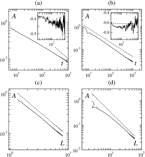
FIG. 2.: Decay of autocorrelation function $A(t,t_{0})$ from single runs of lattices of $4096\times 4096$ as in Fig. 1 ($t_{0}=5$). (a,b): $A$ vs $t$ for parameter sets A and B (logarithmic scales, dashed lines: slope $\lambda/z=5/8$, insets: local slopes); (c,d): $A$ vs $L$ (logarithmic scales) for parameter sets A and B (logarithmic scales, dashed lines: slope $\lambda=5/4$, the quality of the data is not high enough for local slopes).

B Decay of autocorrelation function

Following Zheng, we also measured the decay of the autocorrelation function $A(t,t_{0})=\langle\sigma(t)\sigma(t_{0})\rangle$, but, again, for rather large systems and late times, choosing, in particular, initial reference times $t_{0}$ larger than the “microscopic” transient time. In the usual NCOP phase ordering framework, we expect

$$A(t,t_{0})\sim\left[\frac{L(t_{0})}{L(t)}\right]^{\lambda}\sim\left(\frac{t_{0}}{t}\right)^{\lambda/z}$$

where the Fisher-Huse exponent $\lambda=5/4$. Again, plotting $\log A$ vs $\log t$ for parameter set A may yields an “effective” exponent $\lambda/z$ smaller than its NCOP value (and close to the value given by Zheng), but a closer look reveals a systematic increase of the instantaneous exponent (Fig. 2a and inset). However, plotting $A$ vs $L$, the expected scaling is observed (Fig. 2c). Considering now parameter set B, the expected scaling laws are observed rather easily (Fig. 2b,d). This confirms further that for the parameter values chosen by Zheng, the onset of the asymptotic scaling regime is delayed.

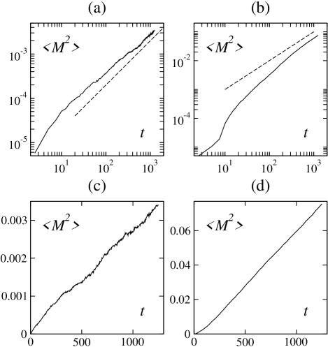
FIG. 3.: Early-time growth of the squared magnetization for an ensemble of 500 symmetric ($M=0$) samples in a lattice of $512\times 512$ sites. (a,b): $\langle M^{2}\rangle$ vs $t$ (logarithmic scales) for parameter sets A and B; dashed lines: slope 1. (c,d): $\langle M^{2}\rangle$ vs $t$ (linear scales) for parameter sets A and B.

C Early-time growth of squared magnetization

For the sake of completeness, and in order to probe the validity of the early-time scaling approach taken by Zheng, we also performed numerical simulations to measure the short-time growth of the squared magnetization $M^{2}$ ($M$ being defined as the spatial average of either $\phi_{i}$ or $\sigma_{i}={\rm sign}(\phi_{i})$) for samples with zero initial magnetization. In this case, for NCOP scaling, we expect $\langle M^{2}\rangle\sim t^{d/z}=t$. Our data on logarithmic scales barely reaches the expected behavior at $t\simeq 10^{3}$ (Fig. 3a,b). Note that the corrections have different sign for the two parameter sets. On linear scales, however, our data reveals the expected proportionality of $\langle M^{2}\rangle$ and $t$ (Fig. 3c,d).

II Corrections to scaling: energy conservation and lattice effects

The above results show that domain growth in the microcanonical $\phi^{4}$ model eventually falls into the NCOP universality class ($z=2$, $\lambda=5/4$) after some possibly long transient behavior. In this section, we suggest that there are two main factors at the origin of these corrections to scaling: space discretization and energy conservation.

A Lattice effects

For the sets of parameters studied by Zheng (notably parameter set A), domain growth initially appears to be slower than the expected NCOP law (the effective value of $z$ measured at short times is larger than two).

This is similar to earlier observations on coupled map lattices, both for the NCOP and COP cases. First measurements of domain growth seemed to indicate slower growth in those discrete-space, discrete-time chaotic models [7, 9], but it was shown later that this non-trivial scaling is only transient and that, for late-enough times, normal scaling is recovered [8, 10]. It was also argued that these long transients gradually disappear in the continuous-space limit which is well-defined in these systems [13].

Here, it is easy to observe that, increasing $g$ (and $m^{2}$, since there is only one free parameter), the slowing-down of domain growth due to lattice effects diminishes, as suggested by the difference between parameter sets A and B. For parameter set B, the transient actually presents faster growth than asymptotically: corrections to scaling are dominated by another phenomenon, stronger than lattice effects.

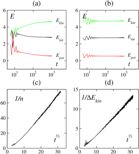
FIG. 4.: Corrections to scaling due to energy conservation. Results for parameter set B, for which these corrections are dominant (see text). (a): the three components of the total energy during phase ordering. (b): same but from ordered initial conditions. (c): decay on the number of interfacial sites (defined as sites with a least one nearest-neighbor of opposite sign); the number of interfacial sites measured during the evolution from an initially-homogeneous configuration has been substracted. (d): Convergence of the total kinetic energy (temperature) towards its asymptotic value: $1/\Delta E_{\rm kin}$ vs $\sqrt{t}$ during phase ordering.

B Energy fluxes

The (conserved) total energy in the system can be partitioned into three components, kinetic, potential, and interaction energy:

$$E_{\rm kin} = \sum_{i}\frac{1}{2}\dot{\phi_{i}}^{2}$$

$$E_{\rm pot} = \sum_{i}-\frac{1}{2}m^{2}\phi_{i}^{2}+\frac{g}{4!}\phi_{i}^{4}$$

$$E_{\rm int} = \sum_{i}\frac{1}{2}\sum_{j=1}^{d}(\phi_{i+j}-\phi_{i})^{2}\;.$$

As domain growth proceeds following random initial conditions, the interaction energy decreases with time as a large part of it is contained in the interfaces separating domains, the density of which decreases like $1/\sqrt{t}$. Potential decreases and kinetic energy increases (Fig. 4).

Starting from “ordered” initial conditions (all sites in the same phase, e.g. $\forall i\;\phi_{i}(0)>0$), the three components of the total energy are almost constant, except for a slight (quasi logarithmic in time) increase of interaction energy and decrease of potential energy due to the nucleation of “thermal” droplets and to relaxation further into potential wells. This effect is indeed larger for parameter set A for which the minimal possible energy density $\epsilon_{\rm min}$ is further away from the critical energy density, leading to stronger thermal fluctuations than for parameter set B.

C Corrections to effective temperature

Kinetic energy can be interpreted as a temperature in the microcanonical context [3]. We can thus see the observed increase of kinetic energy as an increase of the temperature of the system. For the (canonical) Ising model, it is well known [14] that the prefactor of the growth law of $L(t)$ decreases to zero as the temperature approaches its critical value. We suggest to see the growth law observed here for the $\phi^{4}$ model as including a “temperature-dependent” prefactor:

$$L(t)\simeq K(E_{\rm kin})\,\sqrt{t}$$ (1)

Quantitatively (Fig. 4), the kinetic energy seems to reach its asymptotic value like:

$$\Delta E_{\rm kin}\equiv E_{\rm kin}(t)-E_{\rm kin}(\infty)\sim t^{-1/2}$$ (2)

Assuming its analyticity, we can write the prefactor $K$:

$$K(E_{\rm kin})=K_{\infty}+K^{\prime}_{1}\,\Delta E_{\rm kin}+K^{\prime}_{2}\,(\Delta E_{\rm kin})^{2}+\ldots$$ (3)

where $K_{\infty}$ is the asymptotic ($t\to\infty$) prefactor of the domain growth law. Injecting (2) and (3) into (1), we finally expect the following Ansatz to hold for the domain growth law:

$$L(t)=K_{\infty}\sqrt{t}+K_{1}+\frac{K_{2}}{\sqrt{t}}+\ldots$$ (4)

Equation (4) provides excellent fits to our data for the growth of $L(t)$. We find $K_{\infty}\simeq 0.2$, $K_{1}\simeq 2.0$, and $K_{2}\simeq-3.5$ for parameter set A (with $\chi^{2}=7.8$ and correlation coefficient 0.99996) , and $K_{\infty}\simeq 2.1$, $K_{1}\simeq-5.6$, and $K_{2}\simeq 5.7$ (with $\chi^{2}=10^{5}$ and correlation coefficient 0.9997) for parameter set B.

The corrective terms have opposite signs in both cases: this indicates that Eq. (4) is only relevant for parameter set B, because, in analogy with the Ising model, only negative values of $K_{1}$ are allowed (the prefactor of the growth law decreases with increasing temperature). A first conclusion is thus that the main corrections to scaling for parameter set A (typical of those used by Zheng) are due to lattice effects and are not consequences of the conservation of global energy. We note that, similarly, a fit of domain growth in coupled map lattices also yields positive values of $K_{1}$, indicating that this sign is a signature of lattice effects [8].

On the other hand, the above framework does provide the relevant explanation for the corrections to scaling observed for parameter set B, which can thus be traced back to the fluxes between the various components of the energy induced by the decrease of interfaces between domains as phase-ordering proceeds.

III Conclusion

In this Comment, we have shown that Zheng reached erroneous conclusions when studying phase ordering in the microcanonical lattice $\phi^{4}$ model. This system, like other chaotic, deterministic, dynamical systems presenting phase ordering, does display the expected domain growth scaling laws, i.e. those of the non-conserved order parameter case (model A, $z=2$, $\lambda=5/4$). We have shown further that the main influence of the conservation of energy is to introduce corrections to scaling, but that the long transients which plagued Zheng’s approach are due to lattice effects.

Zheng offered, as an explanation for his non-conventional results, that the system considered falls into the class of model C, where a conserved density is coupled to the order parameter [11]. Studies of phase-ordering in model C [16, 17, 15] show that model B-like, but also model A-like behavior can be observed. In this context, the microcanonical $\phi^{4}$ lattice can be considered as a model C system quenched into its “bistable region” (where $z=2$ is observed [18, 15]).

We thank A. Lemaître and A. S. Somoza for interesting discussions and L. Casetti for providing a sample version of his program.

REFERENCES

- [1] E. Fermi, J. Pasta, and S. Ulam, in Collected papers of Enrico Fermi, edited by E. Segré (University of Chicago, Chicago, 1965).
- [2] L. Caiani, L. Casetti, C. Clementi, G. Pettini, M. Pettini, and R. Gatto, Phys. Rev. E 57, 3886 (1998); and references therein.
- [3] L. Caiani, L. Casetti, and M. Pettini, J. Phys. A 31, 3357 (1998).
- [4] B. Zheng, M. Schulz, and S. Trimper, Phys. Rev. Lett. 82, 1891 (1999).
- [5] B. Zheng, Phys. Rev. E 61, 153 (2000).
- [6] A. J. Bray, Adv. Phys. 43, 357 (1994).
- [7] A. Lemaître and H. Chaté, Phys. Rev. Lett. 82, 1140 (1999).
- [8] J. Kockelkoren, H. Chaté, and A. Lemaître, Physica A, 288, 326 (2000).
- [9] L. Angelini, M. Pellicoro, and S. Stramaglia, Phys. Rev. E 60, R5021 (1999).
- [10] J. Kockelkoren and H. Chaté, Phys. Rev. E 62, 3004 (2000).
- [11] P.C. Hohenberg and B.I. Halperin, Rev. Mod. Phys. 49, 436 (1977).
- [12] L. Casetti, Physica Scripta 51, 29 (1995).
- [13] A. Lemaître and H. Chaté, Phys. Rev. Lett. 80, 5528 (1998); J. Stat. Phys. 96, 915 (1999).
- [14] See, e.g., M.-D. Lacasse, M. Grant, and J. Viñals, Phys. Rev. B 48, 3661 (1993).
- [15] J. Kockelkoren and H. Chaté, Physica D 168-169, 80 (2002)
- [16] T. Ohta, K. Kawasaki, A. Sato, and Y. Enomoto, Phys. Lett. A, 126, 93 (1987).
- [17] A. Chakrabarti, J.B. Collins, and J.D. Gunton, Phys. Rev. B 38, 6894 (1988).
- [18] K.R. Elder, B. Morin, M. Grant, and R.C. Desai, Phys. Rev. B 44, 6673 (1991).
- [19] Since is precisely defined as the midheight value of , it is in our opinion not so surprising that we obtain already a good collapse before the scaling regime sets in. In this sense our appoach is different from that of Zheng who tried to collapse .
- [20] Of course, plotting the quantity of interest against and looking for a straight line is not the most accurate way of determining (here we use this only because the log-log plots do not exhibit a constant asymptotic slope). Nevertheless, the value measured by Zheng can safely be rejected since the local slope of against increases with time (not shown here).