Statistics of a hydrophobic chain near a hydrophobic boundary

Abstract

We study the behaviour of a hydrophobic chain near a hydrophobic boundary in two dimensions, using the decorated lattice model of Berkema and Widom [G.T. Barkema and B. Widom, J. Chem. Phys. 113, 2349 (2000)] to obtain effective, temperature dependent intrachain and chain-boundary interactions. We use these interactions to construct two model hamiltonians which can be solved exactly. Our results compare favorably with preliminary Monte Carlo computations, using the same effective interactions. At relatively low temperatures and at high temperatures, we find that the chain is randomly configured in the ambient water, and detached from the wall, whereas at intermediate temperatures it adsorbs onto the wall in a stretched or partially folded state, again depending upon the temperature, and the energy of solvation.

PACS numbers: 5.50.+q, 64.75.+g, 87.15.Aa

I Introduction

Non-polar molecules placed in water behave as if there were attractive interactions between them, at least within a certain temperature interval. This is the co  called hydrophobic  interaction  and is entropy driven. bennaim ; bennaimmakale Hydrophobic interactions play an important role in biological processes, most prominently in protein folding frau ; karplus ; kill . Although many short proteins are able fold on their own within very short times, others require the help of chaperons to be able to do so. To be able to elucidate the role of chaperons, we believe that it would be useful to understand the behavior of a hydrophobic chain in the presence of a hydrophobic boundary.

In trying to understand the behaviour of a hydrophobic chain in water, one must take into account both the hydrophobic interactions mediated by the orientational entropy of the water molecules, and the configurational entropy of the chain, while respecting its connectivity. To compute the temperature dependent effective interaction potentials between the hydrophobic wall and hydrophobic polymer chain and also between the monomers of the hydrophobic chain, we borrowed the decorated lattice model recently proposed by Widom and coworkers ABBwidom ; Widom ; Widom+Barkema . We will calculate the effective free energy cost of bringing a hydrophobic solute molecule from the bulk to a distance $r$ from the hydrophobic wall within the decorated lattice model in one dimension. This will provide an estimate for the interaction potential between the hydrophobic residues of the polymer chain with the hydrophobic wall in two dimensions. We will use the Mean Field Approximation(MFA) to find the effective interaction between neighboring hydrophobic residues in arbitrary dimension.

To be able to compute the partition function of the hydrophobic chain in the presence of a boundary in two dimensions, we introduce two exactly solvable models, using these effective interactions. The first is a solid on solid (SOS) type of simplification of the allowed configurations of the chain. This allows us to reduce the problem to a one-dimensional lattice model, and use the transfer matrix formalism. The second simplified model again consists of performing exact sums over subsets of allowed configurations to obtain an approximation to the true partition function. Thirdly, we will perform Monte Carlo simulations.

To investigate the thermodynamic properties of the chain we have focussed on the mean distance $\langle r_{\rm cm}\rangle$ from the wall, and the average length $\langle L\rangle$ of the projection of the chain on the boundary.

The paper is organized as follows. In section 2, we outline the lattice model within which the effective hydrophobic interactions are computed. In section 3, we will discuss the various simplified models within which we have performed the sums over the chain configurations. In section 4 we discuss our results.

II MODELLING HYDROPHOBIC INTERACTIONS

A decorated lattice model that mimics the solvent mediated hydrophobic interaction was suggested by Widom and his collaborators ABBwidom ; Widom ; Widom+Barkema ; widom3 . In this model, $q$-state Potts spins, $\{s_{i}\}$, are situated at lattice sites. These represent the polar solvent molecules. They can have any of the $q$ different polarization directions. Hydrophobic molecules(HM) can only be accommodated at interstitial sites, more precisely on the bonds connecting neighboring pairs. Lattice-gas variables, $\{\sigma_{ij}\},\;\;\sigma_{ij}=(0,1)$, located on the bonds $(ij)$, indicate whether an interstitial site is empty or occupied by a HM.

Figure 1: Decorated lattice model. Lattice sites are occupied by water molecules (shown as filled circles); hydrophobic molecules (open cirlces) can only be accommodated at interstitial sites.

Interaction between water molecules and HM is always attractive, because of the dipole-induced dipole interaction. On the other hand water molecules can form short lived tetrahedral structures nemethy ; horne stabilized by hydrogen bonds Kittel , i.e., a type of short ranged order. Because these structures have an open cage like space between them, Canpolat HM can be accommodated there without breaking any hydrogen bonds. Thus, this “ordered” configuration is the minimum energy configuration of water molecules in the presence of HM. If there are no HM between the ordered water molecules, there still is an attractive interaction due to the hydrogen bonds and the dipole-dipole interactions, but the absolute value of the interaction energy is smaller, by precisely the amount contributed by the induced dipole interactions. At higher temperatures, water molecules will tend to be oriented randomly. This state, with no HM intermixed with the water molecules, is chosen as the reference, i.e., the zero level of the energy. When water molecules are randomly oriented, they can still have hydrogen bonds between them, though fewer in comparison to the ordered state. However, unlike the ordered state, there will be less open space between them. To be able to accommodate a HM in a disordered region of water molecules, further hydrogen bonds have to be broken. Thus, the insertion of HM within this disordered phase of water molecules is energetically unfavorable. The Hamiltonian for the water-hydrophobic solute system can be written as Widom+Barkema ,

$$H_{W}\, = \sum_{<ij>}\,\left[\,\delta_{s_{i},s_{j}}\delta_{s_{i},1}\left(\sigma_{ij}\,w\,+\,u\right)\,+\right.$$ (1)

$$\left.\sigma_{ij}\,v\left(1-\,\delta_{s_{i},s_{j}}\delta_{s_{i},1}\right)\right]\,.$$

The interaction energies are ordered thus,

$$w\,<\,u\,<0\,<v\,,$$ (2)

where $v$ may be thought of as the solvation energy of the HM in the disordered state of the water molecules. In this model, the unique ordered state of the tetrahedrally bonded pentamers Canpolat , which is able to accommodate the HM without breaking any hydrogen bonds, is identified with the configuration where all the $s_{i}$ are in the state 1.

We immediately realize that Eq.(1) may be rewritten in terms of two-state variables $t_{i}$, defined by

$$\delta_{s_{i},1}\,=\,t_{i}\,.$$ (3)

where $t_{i}\,=\,\{1,0\}$. In the partition function the multiplicity of the $s_{i}\neq 1$ states can be taken care of by inserting a factor of $(q-1)$ for each Potts spin not in the ordered state, or a term $-\beta(1-t_{i})\ln(q-1)$ into the Hamiltonian, to get, in one dimension,

$$H = \sum_{i}^{N}\left.\{t_{i}t_{i+1}\left[\sigma_{i}(w-u-v)+v\right]+\sigma_{i}\,v\right.$$

$$\left.-\beta^{-1}(1-t_{i})\ln(q-1)\}\right.$$

$$\equiv \sum_{i}^{N}H_{i}[t_{i},t_{i+1},\sigma_{i}]\;\;.$$

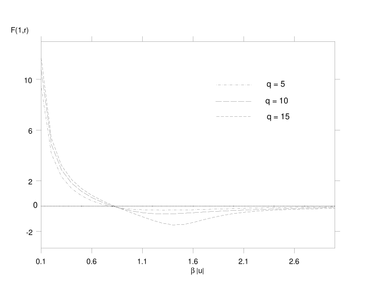
Figure 2: The effective interaction potential of a residue with the hydrophobic wall for different values of $q$, at $r\,=\,1$, at different inverse temperatures. Here $q$ is the number of different orientations which can be assumed by the water molecules. The interaction coefficients of the lattice model were chosen to be $w=-1.5,\;u=-1,\;v=1$.

II.1 Effect of the boundary in 1-d

Let us first consider a one dimensional system, in order to be able to estimate in closed form the effective interaction of a HM with the hydrophobic boundary.

For $N$ being the length of the one-dimensional lattice of water molecules, the free energy cost $F(N,T,r)$ of adding only one HM at an interstitial a distance $r$ from the wall at temperature $T$ is given by

$$-\,\beta F(N,T,r)\,\equiv\,\ln\left(\frac{Z(N,T,r)}{Z_{0}(N,T)}\right)\,,$$ (6)

where $\beta^{-1}=k_{B}T$ as usual, $Z_{0}(N,T)$ is the partition function of the one dimensional system with $\sigma_{i}=0$ for all $i$, that is, no HM molecules, and $Z(N,T,r)$ is the partition function computed in the presence of one HM a distance $r$ from the wall. The effective interaction between the wall and a single HM is thus given by the free energy cost of bringing HM from bulk to distance $r$ from the wall,

$$F_{N}^{(I)}(1,r)\,=\,F(N,T,r)\,-\,F(N,T,r_{b})\,,$$ (7)

where $r_{b}$ means a displacement from the wall beyond which the effect of the wall is no longer perceptible, namely a bulk site. In the thermodynamic limit

$$F^{(I)}(1,r)\,=\lim_{N\to\infty}\,F_{N}^{(I)}(1,r)\;.$$ (8)

To compute the partition functions in (6), we used the transfer matrix method. From Eq.(LABEL:effH), the transfer matrices in one dimension are obtained as

$${\cal T}(\sigma_{i})=\langle t_{i}|e^{-\beta H_{i}[t_{i},t_{i+1},\sigma_{i}]}|t_{i+1}\rangle\;.$$ (9)

Thus, the transfer matrix is conditional on the presence (or absence) of an interstitial HM at each bond connecting two water molecules, and we find,

$${\cal T}(0) = \left(\begin{array}[]{cc}e^{-\beta\,u}&(q-1)^{\frac{1}{2}}\\ (q-1)^{\frac{1}{2}}&(q-1)\end{array}\right)\,,$$ (12)

$${\cal T}(1) = \left(\begin{array}[]{cc}e^{-\beta\,w}&(q-1)^{\frac{1}{2}}\\ e^{-\beta\,v}(q-1)^{\frac{1}{2}}&e^{-\beta\,v}(q-1)\end{array}\right)\,,$$ (15)

for the two possible resulting transfer matrices. ¿From Eq. (7), we get (with one HM inserted at a distance $r$ from the wall),

$$-\beta F_{N}^{(I)}(1,r) = \ln\sum_{k}\langle 1|{\cal T}^{r-1}(0){\cal T}(1){\cal T}(0)^{N-r}\,|k\rangle$$ (16)

$$-\,\ln\sum_{m}\langle 1|{\cal T}^{N-1}(0){\cal T}(1)|m\rangle\,.$$

Notice that the left-most vector is fixed to be unity, signalling the presence of the hydrophobic wall. In the thermodynamic limit $N\to\infty$, this reduces to,

$$-\beta F^{(I)}(1,r) = \ln{\sum_{ijk}A_{i}T_{ij}(1)a_{j1}a_{1k}}$$ (17)

$$-\ln\sum_{ij}a_{11}a_{1j}T_{ji}(1)\;\;,$$

where we have defined

$$A_{i}\equiv a_{11}a_{1i}+\left({\lambda_{2}/\lambda_{1}}\right)^{r-1}a_{21}a_{2i}\;\;\;,$$ (18)

with

$$\lambda_{1,2} \equiv \frac{1}{2}\,e^{-\beta\,u}\left(1+(q-1)e^{\beta\,u}\right.$$ (19)

$$\pm \left.\left[1-(q-1)(2e^{-\beta u}-(q+3)e^{2\beta u})\right]^{\frac{1}{2}}\right)$$

being the eigenvalues of ${\cal T}(0)$, and $a_{kl}$ the elements of its $k$th eigenvector.

The free energy cost of bringing a pair of HMs from the bulk to a distance $r$ from the hydrophobic wall could also be found, similarly, from taking the thermodynamic limit in

$$F^{(I)}(2,r)=\lim_{N\to\infty}F_{N}^{(I)}(2,r)\;,$$ (20)

where,

$$-\beta F_{N}^{(I)}(2,r) = \ln\sum_{k}\langle 1|{\cal T}^{r-2}{\cal T}^{2}(1){\cal T}^{N-r}|k\rangle$$ (21)

$$-\,\ln\sum_{m}\langle 1|{\cal T}^{N-2}{\cal T}^{2}(1)|m\rangle\,,$$

and ${\cal T}(0)$ is to be understood where the argument has been omitted.

We have plotted $F^{(I)}(1,r)$ in Fig. (2) as a function of the inverse temperature. We find that, at intermediate temperatures $F(1,r)$ becomes attractive. Although $F^{(I)}(2,r)$ is always positive, it becomes smaller at intermediate temperatures. Hydrophobic interactions become effective in a temperature interval which can be seen to range approximately between $|u|/(2k_{B})<T<2|u|/k_{B}$.

We will use $F^{(I)}(1,r)$, which we have calculated exactly in one dimension, to give us an estimate of the interaction between the HM and the hydrophobic boundary in two dimensions. On the other hand, to take into account the self-interactions of the chain in two dimensions we also need an effective temperature dependent pair potential. This is the subject of the next section.

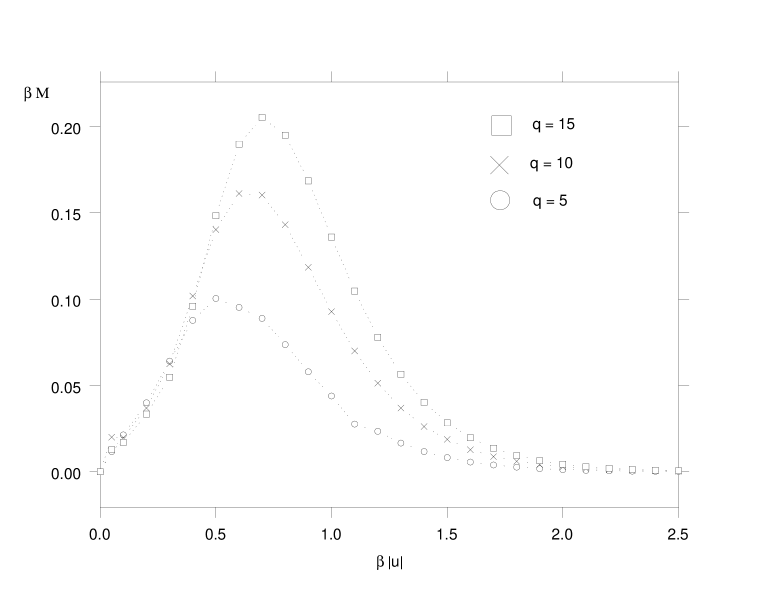
Figure 3: Effective, temperature dependent nn and nnn interaction energies between hydrophobic residues in water, in the MF approximation to the decorated lattice model Widom+Barkema . Different $q$ values are shown. The effective interaction is stronger for larger $q$. The coupling constants for the decorated lattice model are the same as in Fig. 2.

II.2 Effective hydrophobic pair interaction in the Mean Field Approximation

We made use of the Mean Field Approximation (MFA) to find the solvent mediated interaction between the hydrophobic molecules on a cubic latice in arbitrary dimension. In the MFA, the Hamiltonian (1) of a water molecule interacting with neighboring hydrophobes in two dimensions, in the presence of a mean field $\langle t\rangle$ due to the ordering of the ambient water molecules, can be written as,

$$H_{\rm MF} = \,\sum_{j=1}^{2d}\,\{t\langle t\rangle[\sigma_{j}(w-u-v)+u]+\sigma_{j}\,v\}$$ (22)

$$-\beta^{-1}\mu(1-t)\ln(q-1)\,.$$

where $d=2$ and $\mu$ has been inserted for later convenience in computing expectation values, and will be set to unity otherwise. Performing the $t$ sum in the partition function leads to couplings between the $\sigma_{j}$ situated on the bonds emanating from the lattice site on which $t$ is located. We define the effective two-body interaction strength $M$ between the nearest neighbor (nn) and next nearest neighbor (nnn) pairs (which are indistinguishable from each other in this approximation), as well as the four-body (or plaquette) interactions between the HM, via,

$$Z = \sum_{\{\sigma_{i}\},t}e^{-\beta H_{\rm MF}[t,\{\sigma_{i}\}]}$$ (23)

$$= \sum_{\{\sigma_{i}\}}e^{\beta\left[M\sum_{(ij)}\sigma_{i}\sigma_{j}+K\prod_{i=1}^{4}\sigma_{i}\right]}\;\;\;,$$

where $(ij)$ denotes nn and nnn pairs. To the first approximation widom3 we will neglect the plaquette coupling $K$. Keeping only the two-body interactions, we find,

$$e^{\beta M}\, = \frac{e^{-2\beta\,[\langle t\rangle(w-v+u)+v]}\,+\,(q-1)e^{-2\beta\,v}}{\left[e^{-\beta\,[\langle t\rangle(w-v+3\,u)+v]}\,+\,(q-1)e^{-\beta\,v}\right]^{2}}$$ (24)

$$\times \left(e^{-\,4\beta\,u\langle t\rangle}+q-1\right)\,.$$

From

$$1-\langle t\rangle\,=\,\frac{\partial}{\partial\mu}\ln Z|_{\mu=1}$$ (25)

one gets a self-consistent expression for $\langle t\rangle$, which we solved numerically for each given temperature $T$. Substituting in Eq.(24) one finally obtains the effective solute-solute interaction energy in two dimensions, which we plot in Fig.(3) for different choices of $q$. The interaction between HMs is attractive for any finite temperature.

III STATISTICAL MECHANICS OF POLYMER CHAIN

We are interested in the behavior of a hydrophobic polymer chain in the presence of a hydrophobic wall. We used three different approaches.

III.1 Modular chain or SOS model

We define a set of elementary modules, from which a large number of chain conformations can be built, such that only nearest neighbor modules come within the interaction range of each other. The subset of configurations that can be generated by random combinations of the modules that are shown in Figure( 4a) can clearly be seen as graphs (taking the boundary as the axis) without overhangs, as in a restricted solid-on-solid (SOS) model SOS in (1+1) dimensions, where successive steps are constrained to differ by at most one unit of height. Making use of the linearity of the chain and the restriction to nearest neighbor interactions between the modules, we used the transfer matrix along the chain to solve the partition function exactly for our model Hamiltonian.

We labeled the modules in Figure( 4a) as $1$, $2$, $3$ from left to right. A chain configuration is uniquely specified by associating a variable, $u_{i}=\{1,2,3\}$, $i=1,\ldots,N_{m}$, with each module along the chain, and by specifying the distance of the first module from the wall. Note that the number of residues along the chain is given by $2N_{m}$ in this case. The interaction energy of each residue with hydrophobic wall is given in terms of $F^{(I)}(1,r)$. Moreover, we took $M(\beta)$, defined in Eq.(24), to be the interaction energy between nearest and next nearest neighbor residues. (see Fig.(4b)). Note that the nearest neighbor interaction (wavy line) connects residues belonging to modules twice removed from each other. Yet, since this occurs only in the $(i,i+1)=(2,3)$ or (3,2) combination, independently of the identity of the $i-1$st module, it can still be accomodated within a nearest-neighbor Hamiltonian.

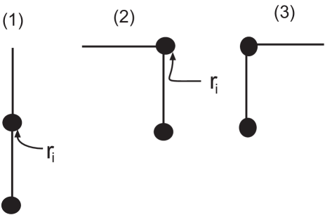
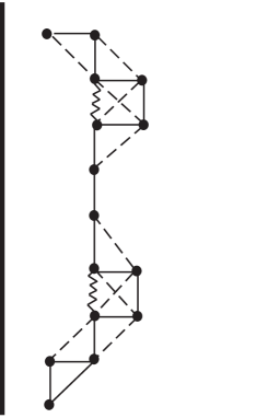
Figure 4: a) (Top panel) Elementary modules used to generate SOS like chain configurations which only allow nearest neighbor interactions between the modules, via nn or nnn interactions between the hydrophobic residues. b) (Lower panel) Nearest and next nearest neighbor interactions $M(\beta)$ between HMs on the chain are indicated as wavy and dashed lines, respectively.

We model the effective Hamiltonian of a polymer with $N_{m}$ modules as,

$$H_{c}=-\sum_{i}^{N_{m}} \left\{M(\beta)\langle u_{i}|\Gamma|u_{i+1}\rangle\right.$$

$$+ \left.h_{1}(r_{i-1},r_{i})+h_{2}(r_{i},u_{i})\right\}\,.$$

The vectors $|u_{i}\rangle$ correspond to the three states of the variable $u_{i}$, i.e., $(1,0,0)$, $(0,1,0)$ etc., so that the coefficient of the pair interaction $M(\beta)$ is conveniently written in terms of

$$\Gamma=\left(\begin{array}[]{ccc}0&2&2\\ 0&2&3\\ 0&3&2\end{array}\right)\,.$$ (27)

The second term is the free energy cost of adding HMs to the solvent matrix, $h_{1}(r_{i})=-F^{(I)}(1,r_{i-1})-F^{(I)}(1,r_{i})$. The distance of the second residue on the $i$th module from the wall, $r_{i}$, is found from $r_{i}=r+\rho_{i}$, where $r$ is the distance of the first module from the wall, and

$$\rho_{i}\,=\,\sum_{j=1}^{i}\,\left(\delta_{u_{j},2}\,-\,\delta_{u_{j},3}\right)\,.$$ (28)

Note that the displacement of the first residue on the $i$th module is the same as that of the second residue on the $i-1$st module, and therefore the expression for $h_{1}$ follows. The final term is

$$h_{2}(u_{i})=-F^{I}(2,r_{i}+1)\delta_{u_{i},2}-F^{I}(2,r_{i}-1)\delta_{u_{i},3}\;\;,$$ (29)

and adds on the extra cost of placing a pair of HM in the same “row” perpendicular to the wall. In practice, we found that the addition of this term overestimates the interaction with the wall. While its inclusion or omission had a minimal effect on the average center of mass displacement from the wall, its inclusion led to unrealistic results for the projected chain length. Therefore in the calculations reported below, it has been set to zero.

The partition function of the polymer is,

$$Z\,=\,\sum_{r}\sum_{\{u\}}\,e^{-\beta\,H_{c}}\,.$$ (30)

Explicitly,

$$Z = \sum_{\{r_{i}\},\{u_{i}\}}\,\langle r_{1},u_{1}|{\cal U}|r_{2},u_{2}\rangle\langle r_{2},u_{2}|{\cal U}|r_{3},u_{3}\rangle\ldots$$ (31)

$$\ldots\langle r_{N_{m}-1},u_{N_{m}-1}|{\cal U}|r_{N_{m}},u_{N_{m}}\rangle\,.$$

Here, $|r_{i},u_{i}\rangle$ are $\mathcal{M}\times 3$ dimensional vectors, with $\mathcal{M}$ being the size of the system in the direction orthoganal to the wall. The transfer matrix ${\cal U}$ is given by a direct product

$${\cal U}=\sum_{\zeta=1}^{3}W^{(\zeta)}\otimes R^{(\zeta)}$$ (32)

with

$$W^{(1)}_{k\ell} = \delta_{\ell,1}$$ (33)

$$W^{(2)}_{k\ell} = \delta_{\ell,2}\left[e^{2\beta M}\left(\delta_{k,1}+\delta_{k,2}\right)+e^{3\beta M}\delta_{k,3}\right]$$ (34)

$$W^{(3)} = (2\leftrightharpoons 3)\;\;,$$ (35)

where $k,\ell=1,2,3$, $(2\leftrightharpoons 3)$ indicates an interchange of the indices 2 and 3 in the previous equation, and

$$R^{(\zeta)}_{\gamma\eta} = \delta_{\zeta,1}\,\delta_{\gamma,\eta}e^{-\,2\beta F^{I}(1,\gamma)}$$ (36)

$$+ \delta_{\zeta,2}\,\delta_{\gamma,\eta-1}e^{-\,\beta\,\left[F^{I}(1,\gamma)+F^{I}(1,\eta)\right]}$$

$$+ \delta_{\zeta,3}(\gamma\leftrightharpoons\eta)\;\;,$$

where $\gamma,\eta=1,\ldots{\cal M}$ and $\zeta=1,2,3$. We note that only the diagonal, upper diagonal and lower diagonal elements of the matrices $R^{(\zeta)}$ are different from zero.

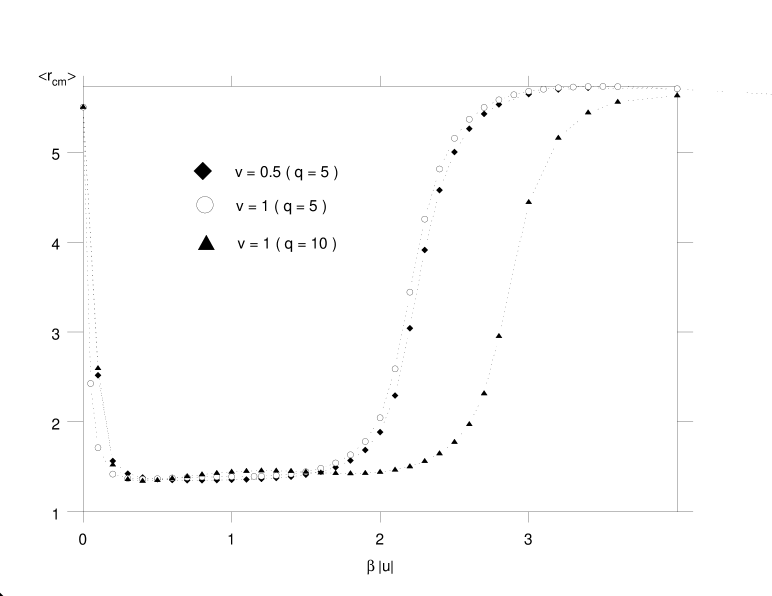
Figure 5: The average center of mass displacement from the boundary, of the hydrophobic chain with $60$ residues in the SOS approximation, for different values of solvation energy, $v$, and different values of $q$. For computational purposes, the width of the channel was chosen to be 12 lattice spacings.

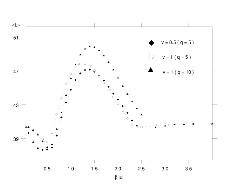
Figure 6: Mean length of the hydrophobic chain with $60$ residues, projected on to the boundary, in the SOS approximation. Different values of solvation energy, $v$, and different values of $q$ are shown for comparison.

We calculated the center of mass distance,

$$\langle r_{\rm cm}\rangle={1\over N_{m}}\left\langle\sum_{i}^{N_{m}}r_{i}\right\rangle\;,$$ (37)

of the hydrophobic polymer from the hydrophobic boundary as a function of temperature, and this is shown in Fig.(5). At intermediate temperatures the polymer chains are attracted to the wall so strongly that $\langle r_{\rm cm}\rangle\simeq 1.5$. The chains are predominantly in a zig-zag configuration confined very close to the wall, with half of them actually adsorbed on the wall, and the maximum number of nn and nnn interactions.

As $\beta\to 0$ (high temperatures) the intrachain interactions $M$ also go to zero, the entropy of the chain becomes the determining factor, and the chain floats free. At low temperatures, as the entropy term in the free energy becomes negligible, the equilibrium state is determined by energetic considerations, and the polymers desorb and take on random configurations, constraining a large number of water molecules in their neighborhood.

The average end to end distance of the polymer chain, projected on to boundary, is given by

$$\langle L\rangle=N_{m}+\left\langle\sum_{i}^{N_{m}}\delta_{u_{i},1}\right\rangle\;\;.$$ (38)

The temperature dependence is reported in Fig. (6). In the limit $\beta\to 0$, clearly $\langle L\rangle=N_{m}(1+1/3)$, which is what one sees in Fig.(6), with $N_{m}=30$. It is interesting to note the non-monotonic behaviour of $\langle L\rangle$ within the region of interest, namely the temperature interval for which the center of mass lies very close to the wall. This non-monotonicity arises from the competition between the entropy mediated effective self-interaction of the chain (leading to smaller $L$) and the interaction with the wall (completely shielding one side from the water by stretching out to adsorb on to the wall). This behaviour is also observed in the models we have considered in the subsequent sections.

Although the SOS model is exactly solvable, it is unable to take into account configurations of the chain which fold on themselves, and we therefore have also considered a model where such conformations are allowed.

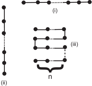
Figure 7: Polymer configurations included in the exact enumeration of the $n$-fold model.

III.2 The $n$-fold model

In this section we take a different tack, and perform exact summations over a richer conformation set for the same interactions, although this still includes only a fraction of all possible polymer configurations. These configurations are shown in Fig.(7). If the length of the polymer is $N_{l}$ then the energy of a chain with an integer number of folds $N_{l}/n$, is given by

$$H_{n}\,=\,\frac{N_{l}}{n}\sum_{i=1}^{n}F^{(I)}(1,r+i)\,-\,M\,\nu_{n}(1-\delta_{n1}-\delta_{nN_{l}})$$ (39)

where $r$ is the distance from the wall (see Fig.(7)) and $\nu_{n}$ is the total number of nearest neighbor and next nearest neighbor pairs in this configuration, $\nu_{n}=3(n-1)(N_{l}/n-1)$. We calculated $\langle L\rangle=\langle N_{l}/n\rangle$, which is the mean value of the vertical distance between the first and last monomer, from

$$\langle N_{l}/n\rangle\,=\,\frac{1}{Z}\sum_{r}\sum_{n}^{{}^{\prime}}\,\frac{N_{l}}{n}\,e^{-\beta\,H_{n}}\,.$$ (40)

where the prime indicates that the summation is only over the subset of configurations described above, with $N_{l}/n$ integer. We also calculated the center of mass displacement from the wall, $\langle r_{\rm cm}\rangle$. These quantities are shown in Figs.(8,9).

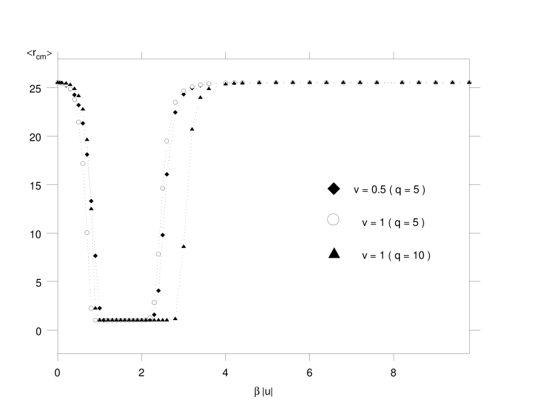
Figure 8: The average center of mass displacement from the wall, of a polymer with $50$ residues, for different values of the solvation energy, $v$, and of $q$, in the $n$-fold model. The width of the channel was taken to be 50 lattice units.

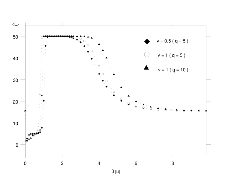
Figure 9: The average longitudinal component of the length of the hydrophobic polymer with $50$ residues, for different values of solvation energy, $v$, and of $q$, in the $n$-fold model.

In the low temperature limit, increasing the number of HM-water nn pairs lowers the energy and this is favorable since the entropy term in the free energy is suppressed, and the chain takes on relatively open, random configurations. At intermediate temperatures where the hydrophobic interactions are the most effective, the chain prefers to neighbor the hydrophobic wall at as many nn sites as possible, and therefore is adsorbed on the wall in the unfolded state. As the temperature is raised somewhat more, effective self interactions of the chain become more important, and the chain is in a more folded state, although still adhering close to the wall. At high temperatures it is advantageous to minimize the number of nearest neighbor sites at which the chain is in contact with water molecules, since the entropy of the water molecules is rather large, especially for large $q$. On the other hand, the entropy of the chain also favors open configuration, which wins out in the high temperature limit. It should be noted that in Fig. (9), with $N_{l}=50$, $\langle L\rangle$ is close to $N_{l}^{3/4}=18.8$, at both extremes, with the power being that of the Self Avoiding Walk in two dimensions.

III.3 Monte Carlo simulations

For comparison, we display in Figs.(10,11) preliminary Monte Carlo simulation results, for 3$\times 10^{5}$ random Self Avoiding Walk configurations of length $N=20$. The initial points of the walks have been randomly chosen within a $100\times 100$ square lattice. If a random walk passes through any lattice point which it has already visited, the configuration is discarded, and a new one generated. Each successfully generated configuration was decorated with the interaction potentials found in section (II), namely, $F^{(I)}(1,r)$ and $M(\beta)$ (Eqs.( 7,24)), to finally compute the expectation values for the center of mass displacement from the wall and the longitudinal component of the end to end distance, in the canonical ensemble. We will be reporting on more extensive Monte Carlo simulations in a separate publication.

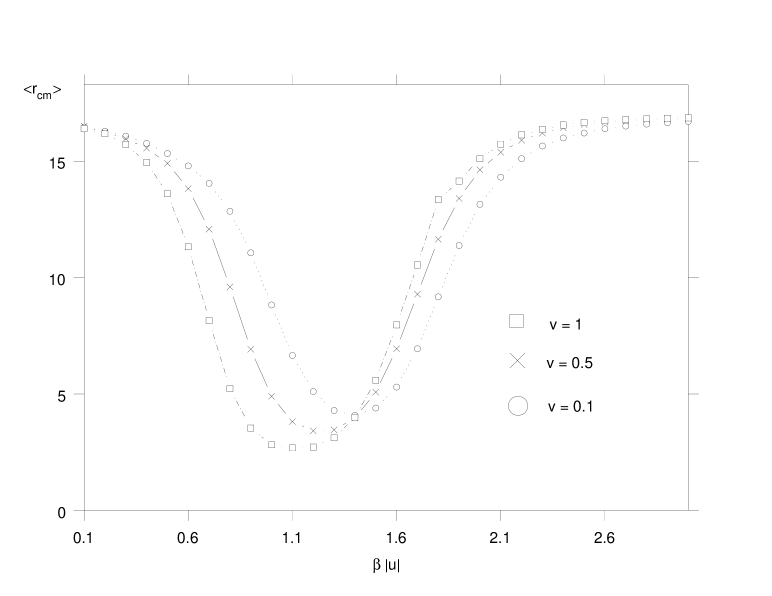
Figure 10: Preliminary Monte Carlo results for average center of mass displacement of the hydrophobic chain from the hydrophobic boundary, for different values of solvation energy, $v$. The chain length is 20 residues, and the channel size is 100 lattice spacings.

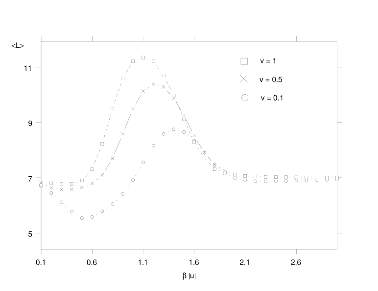
Figure 11: Same as in Fig. 10, for the projection of the end to end distance of the hydrophobic chain on the boundary, for different values of the solvation energy, $v$.

IV Discussion

We have presented two exactly solvable versions of a model for the statistics of a hydrophobic polymer chain in water, in the presence of a hydrophobic boundary. The model of Widom and co-workers ABBwidom ; Widom ; Widom+Barkema for hydrophobic interactions has been our point of departure for computing approximate effective intrachain and chain-boundary potentials. Although the behaviour of chains (or membranes) in the vicinity of spatial boundaries have been considered before Netz ; Stella ; Eisenriegler , these studies have concentrated on temperature independent interactions.

With the inclusion, to various degrees of accuracy, of the entropy of the chain, we are able to take into account the competition between the entropy of the water molecules which can be constrained by the presence of hydrophobic molecules in their neighborhood, and the entropy of the chain. We find that although at low and high temperatures, the chain prefers to be in a random configuration, detached from the wall, there is an intermediate temperature range where it is adsorbed on to the wall, at least for the relative values of the hydrogen bond, dipole-induced dipole and solvation energies which we have assumed. For relatively smaller values of the solvation energy, $v$, there is a sub-interval of temperatures, where the chain adheres to the wall in a relatively folded state. It is gratifying to find that this qualitative feature found in the exactly soluble SOS model and the $n$-fold model is reproduced in the Monte Carlo calculation, although the adsorbed “phase” occurs at somewhat higher temperatures.

The present study provides one way of modelling the interaction of a protein with a hydrophobic surface. Our results are interesting from the point of view of protein dynamics, especially for the folding of relatively long polymer chains, which may need the assistance of chaperons to fold correctly. Kim The effect of hydrophobic boundaries on the folding of amino-acid chains is also interesting from an evolutionary point of view, as has been suggested by Tüzel and Erzan ETAE . Further work is in progress, to include polar as well as hydrophobic elements, for a more realistic protein chain.

Acknowledgements

It is a pleasure to acknowledge a useful discussion with Nihat Berker. One of us would like to acknowledge partial support from the Turkish Academy of Sciences.

References

- (1) A. Ben-Naim, Hydrophobic Interactions (Plenum, New York and London, 1980)
- (2) A. Ben-Naim, J. Chem. Phys., 90(12), 7412 (1989)
- (3) H. Frauenfelder,S.G. Sligar,P.G. Wolynes, Science, 254, 1598 (1991)
- (4) A. Sali, E. Shakhnovich, J. Mol. Biol., 235, 1614-1636 (1994)
- (5) K.A. Dill et al., Protein Science, 4, 561-602 (1995)
- (6) A.B. Kolomeisky, B. Widom, Faraday Discuss.,112, 81-89 (1999)
- (7) B. Widom, Pol. J. Chem., 75, 507 (2001)
- (8) G.T. Barkema and B. Widom, J. Chem. Phys., 113, 2349 (2000)
- (9) D. Bedeaux, G.J.M. Koper, S. Ispolatov, B. Widom, Physica A 291, 39 (2001).
- (10) G. Némethy, H.A. Scheraga, J. Chem. Phys., 36, 3382 (1961)
- (11) R.A. Horne ed., Water and Aqueus Solutions Structure, Thermodynamics, and Transport Processes (John Wiley & Sons, London, 1972)
- (12) C. Kittel, Introduction to Solid State Physics (John Wiley & Sons,Inc., 1986)
- (13) M. Canpolat, F.W. Starr, A. Scala, M.R. Sadr-Lahijany, O. Mishima, S. Havlin, H.E. Stanley, Chem. Phys. Lett., 294, 9 (1998); H.E. Stanley , S.V. Buldyrev, M. Canpolat, O. Mishima, M.R. Sadr-Lahijany, Physica A 257, 213 (1998) and Phys. Chem. Chem. Phys. 2, 1551 (2000).
- (14) G.H. Gilmer and P. Bannema, J. Appl. Phys. 43, 1347 (1972); H. van Beijeren, Phys. Rev. Lett. 38, 993 (1977); for a review see D.B. Abraham, in Phase Transitions and Critical Phenomena, Vol. 10, C. Domb and J. Lebowitz eds., (Academic Press, N.Y. 1986).
- (15) R.R. Netz, D. Andelman, Oxide Surfaces (Marcel Dekker Inc., New York, 2000)
- (16) A. Stella, T. Jr. Phys., 18, 224 (1994).
- (17) E. Eisenriegler, Polymers near surfaces (World Scientific, Singapore, 1993).
- (18) J.D. Bryngelson, E.M. Billings, Physics of Biological Systems (Springer, Berlin, 1997)
- (19) E. Tüzel, A. Erzan, “A Thermodynamic Model for Prebiotic RNA - Protein Co-evolution,” (unpublished).