Itinerant Ferromagnetism in the Periodic Anderson Model

Abstract

We introduce a novel mechanism for itinerant ferromagnetism, based on a simple two-band model. The model includes an uncorrelated and dispersive band hybridized with a second band which is narrow and correlated. The simplest Hamiltonian containing these ingredients is the Periodic Anderson Model (PAM). Using quantum Monte Carlo and analytical methods, we show that the PAM and an extension of it contain the new mechanism and exhibit a non-saturated ferromagnetic ground state in the intermediate valence regime. We propose that the mechanism, which does not assume an intra atomic Hund’s coupling, is present in both the iron group and in some $f$ electron compounds like Ce(Rh_1-xRu_x)₃B₂ , La_xCe_1-xRh₃B₂ and the uranium monochalcogenides US, USe, and UTe.

I Introduction

Itinerant ferromagnetism was the first collective quantum phenomena considered as a manifestation of the strong Coulomb interactions which are present in an electronic system. However, the origin of this phenomenon is still an open problem. Here we introduce a novel mechanism for itinerant ferromagnetism, which is based on a simple two-band model. This work is an extension of a previous letter [1] where we have described the basic ideas. In this paper, we show that the mechanism is supported by the numerical results obtained from quantum Monte Carlo (QMC) simulations of the periodic Anderson model (PAM). We also analyse the experimental consequences for some $f$ electron compounds and the Iron group. However, before describing the details of our mechanism, it is useful to develop a historical perspective for the itinerant ferromagnetism.

Seventy four years ago, Heisenberg [2] formulated his spin model to address the problem of ferroamgnetism, but as Bloch [3] pointed out, a model of localized spins cannot explain the metallic ferromagnetism observed in iron, cobalt and nickel. By introducing the effects of exchange terms into the Sommerfeld description of the free-electron gas, Bloch predicted a ferromagnetic ground state for a sufficiently low electron density. In 1934, Wigner [4] added the correlation terms to the model considered by Bloch. After analyzing the effects of the correlations, he concluded that the conditions for ferromagnetism in the electron gas were so stringent as to be never satisfied.

The first attempt at analyzing a real FM metal, like Ni, was made by Slater [5]. He concluded that the main contribution to the exchange energy is provided by intra-atomic interactions. In the meantime, Stoner [6] introduced his picture where the metallic ferromagnetism results from holes in the $3d$ band interacting via an exchange energy proportional to the relative magnetization and obeying Fermi-Dirac statistics. However, the model considered first by Stoner [6] and later by Wohlfarth [12], did not take into account the correlations of the $3d$ electrons, except for the constraints imposed by the Pauli exclusion principle. In other words, they did not consider the fact that the Coulomb repulsion tends to keep the electrons apart.

In 1953, the importance of these correlations was pointed out by van Vleck [15]. He emphasized that the energy required to tear off an electron increases rapidly with the degree of ionization. (The energy of two Ni atoms in a $3d^{9}$ configuration is appreciably lower than having one atom in the $3d^{8}$ state and the other one in $3d^{10}$.) Based on this observation, he proposed an alternative picture (minimum polarity model) where the states of higher ionization in Ni are ruled out completely, and the configuration $3d^{9.4}$ is considered to be 40 percent $3d^{10}$ and sixty percent $3d^{9}$. The lattice sites occupied by $3d^{9}$ and $3d^{10}$ configurations are continuously redistributing in his picture. The van Vleck proposal is the precursor of the Hubbard model for infinite $U$.

Following Slater [14], van Vleck [15] speculated that the contamination by states of higher polarity, not included in his model, provides the exchange interaction (intra-atomic in this case) necessary for ferromagnetism. Hence he calculated the effective nearest-neighbor magnetic interaction induced by second order perturbative fluctuations from the $d^{9}+d^{9}$ configuration to the $d^{8}+d^{10}$. In this way, van Vleck arrived at a model which describes itinerant and correlated (only allowing $d^{9}$ and $d^{10}$ configurations) holes with a nearest-neighbor exchange interaction $\alpha{\bf S_{i}.S_{j}}$ (generalized Heisenberg model). However, as van Vleck explained at the end of his paper [15], the sign and the magnitude of $\alpha$ are very sensitive to the precise values of the energies of the different possible intermediate states (singlets or triplets) in the $d^{8}$ configuration.

In 1963, the one-band Hubbard model was proposed independently by Gutzwiller [16], Hubbard [17] and Kanamori [18] to explain the metallic ferromagnetism in the $3d$ transition metals. The Hubbard model incorporates the kinetic energy in a single nondegenerate band with an intra-atomic Coulomb repulsion $U$ to describe the electrons in the $s$ band of the transition metals. In contrast to the previous models, the Hubbard model does not include any explicit exchange interaction which favors a ferromagnetic phase. The implicit question raised by this proposal is: Can ferromagnetism emerge from the interplay between the kinetic energy and the Coulomb repulsion, or it is strictly neccesary to include an explicit exchange interaction provided by the intra-atomic Hund’s coupling? This simple question becomes even more relevant if we consider $f$-electron itinerant ferromagnets, like CeRh₃B₂ [19], whose only local magnetic coupling is antiferromagnetic.

Unfortunately, with the exception of Nagaoka’s [20] and Lieb’s [21, 22] theorems, the subsequent theoretical approches were not controlled enough to determine whether the Hubbard model has a FM phase. The central issue is the precise evaluation of the energy for the paramagnetic (PM) phase. Because it does not properly incorporate the correlations, mean field theory overestimates this energy and predicts a large FM region [23]. In contrast, numerical calculations have narrowed the extent of this phase to a small region around the Nagaoka point [20].

There are several controversies in the history of itinerant ferromagnetism. Most of them originate in the lack of reliable methodologies to solve strongly correlated Hamiltonians. In addition, the number of compounds exhibiting ferromagnetism has increased during the last several decades. There is a new list of $Ce$ and $U$ based compounds which are itinerant ferromagnets [24] with large Curie temperatures (of the order of 100^∘K) and the only explicit magnetic interaction is antiferromagnetic (Kondo like). This observation stimulated us to reconsider the situation of the iron group and ask whether the ferromagnetism originates in the intra-atomic Hund’s interaction or is just a consequence of the strong Coulomb repulsion between electrons with a particular band structure. One possible and plausible alternative is that these two phenomena are cooperating to stabilize a ferromagnetic ground state. In any case, it is important to elucidate whether a realistic lattice model only containing repulsive terms (for instance, the Hubbard model) can sustain a ferromagnetic state, or it is necessary to invoke additional terms which are explicitly ferromagnetic. The Hubbard Hamiltonian is in the first category. However, the most accurate numerical calculations seem to indicate that this model does not sustain a ferromagnetic ground state.

Going beyond the simple one-band Hubbard model has been advocated, for instance, by Vollhardt et al [23]. They note that the inclusion of additional Coulomb density-density interactions, correlated hoppings, and direct exchange interactions favors FM ordering in the single-band Hubbard model. In fact, a very simple analysis shows that increasing the density of states ${\cal D}(E)$ below the Fermi energy $E_{F}$ and placing $E_{F}$ close to the lower band edge increases the FM tendency. One can achieve this by including a next nearest neighbor hopping $t^{\prime}$ or by placing the hoppings on frustrated (non-bipartite) lattices. The effectiveness of $t^{\prime}$ was studied numerically by Hlubina et. al. [25] for the Hubbard model on a square lattice. They found a FM state when the van Hove singularity in ${\cal D}(E)$ occurred at $E_{F}$. However, this phase was not robust against very small changes in $t^{\prime}$.

After seven decades of intense effort, the microscopic mechanisms driving the metallic FM phase are still unknown [23, 28]. We still do not know what is the minimal lattice model of itinerant ferromagnetism and, more importantly, the basic mechanism of ordering.

While the Hubbard model is so reluctant to have a FM state, there is an increasing amount of evidence indicating that the Periodic Anderson Model (PAM) has a FM phase in a large region of its quantum phase diagram [1, 29, 30, 31, 32, 33, 34, 35, 36, 37, 38, 39]. Since the $d$ orbitals of the transition metals are hybridized with the $s-p$ bands, we can consider the inclusion of a second band as the next step in the search of itinerant ferromagnetism from pure Coulomb repulsions. Indeed a very simple extension of the PAM can be used to describe the physics of the iron group [40, 30]. In addition, there is large number of cerium and uranium compounds, like Ce(Rh_1-xRu_x)₃B₂ ($T_{c}=115K$) [41, 42], CeRh₃B₂ [19], and US, USe, and UTe [24] which are metallic ferromagnets and can be describred with the PAM.

Ferromagnetism is readily found in the PAM by mean-field approximations in any dimensions [33, 34, 35, 36, 37, 38, 39]. Using a slave-boson mean-field theory (SBMFT) for the symmetric PAM, Möller and Wölfe [33] found a PM or antiferromagnetic (AF) phase at half filling depending on the value of the Coulomb repulsion $U$. By lowering the density of electrons from 1/2 filling, they also found a smooth crossover from AF to FM order via a spiral phase. Just before 1/4 filling, they got a first-order transition from FM to AF order. More recently, the SBMFT calculations of Doradziński and Spalek [34, 35] found wide regions of ferromagnetism in the intermediate valence regime that surprisingly extended well below 1/4 filling.

A ferromagnetic phase is also obtained when the dynamical mean-field theory (DMFT) is applied to the PAM [36, 37, 38, 39]. Tahvildar-Zadeh et al. found a region of ferromagnetism and studied its temperature dependence. At very low temperatures, their ferromagnetic region extended over a wide range of electron fillings and in many cases embraced the electron filling of 3/8. They proposed a specific Kondo-induced mechanism for ferromagnetism at 3/8 filling that has the conduction electrons in a spin-polarized charge density-wave anti-aligned with the ferromagnetically aligned local moments on the valence orbitals. More recently Meyer and Nolting[37, 38, 39] appended perturbation theory to DMFT and also predicted ferromagnetism over a broad range of electron filling extending below 1/4 filling. In addition Schwieger and Nolting [43] also considered an extension of the PAM, similar to the one considerd here, to estimate the importance of $s-d$ hybridization for the magnetic properties of transition metals.

There is also a considerable amount of numerical evidence showing ferromagnetic solutions for the ground state of the PAM. Noack and Guerrero [31], for example, found partially and completely saturated ferromagnetism using the density matrix renormalization group (DMRG) method in one dimension. They considered a parameter regime where there is one electron in each $f$ orbital. For a sufficiently large value of $U$, the model exhibited a ferromagnetic ground state. Beyond an interaction-dependent value of the doping and a doping-dependent value of $U$, this state disappeared. The ferromagnetic phase was a peninsula in a phase diagram that was otherwise a sea of paramagnetism except at 1/4 and 1/2 filling where the ground state of the PAM was antiferromagnetic.

Our previous [29] and new QMC results qualitatively agree with the DMRG work; however, the phases we find quantitatively and qualitatively disagree with those derived from the mean-field approximations. Quantitatively, we find ferromagnetism in a narrower doping range than the one predicted by the DMFT and SBMFT calculations. For fillings between 3/8 and 1/2, QMC predicts a PM region, whereas mean-field theory predicts ferromagnetic states in part of that region. In fact, at a filling of 3/8 where DMFT calculations predict ferromagnetism, we find a novel ground state of an entirely different symmetry. Instead of ferromagnetism, QMC finds a resonating spin density-wave (RSDW) state; that is, the ground state was a linear combination of two degenerate spin-density waves characterized by the $(\pi,0)$ and $(0,\pi)$ wave vectors.

The novel mechanism we introduce in the present paper operates when the system is in a mixed valence regime. This regime has been studied numerically only in the context of DMFT [37]. We will show however that the ferromagnetic solution obtained with DMFT in the mixed valence regime has a different origin and therefore is not representative of our new mechanism. The main ingredients for our mechanism are an uncorrelated dispersive band which is hybridized with a correlated and narrow band. We show the PAM supports our mechanism by doing quantum Monte Carlo (QMC) simulations on one and two dimensional lattices. The results of these simulations are interpreted with an effective Hamiltonian derived from the PAM. In this way, we establish that the new mechanism can be interpreted as a generalization to the lattice of the first Hund’s rule for the atom. The two level band structure generated by the gap recreates for the lattice, the shell-like level strucure of the hydrogenic atom. When the lower shell is incomplete, the local part of the Coulomb interaction is minimized by polarizing the electrons which are occupying the incomplete shell.

II Model

The PAM was originally introduced to explain the properties of the the rare-earth and actinide metallic compounds including the so called heavy fermion compounds. A very simple extension of this model can also be applied to the description of many transition metals [26, 40]. The basic ingredients of this model are a narrow and correlated $f$ band hybridized with a despersive and uncorrelated $d$ band. The Hamiltonian associated with this model is:

$$H=H_{0}+H_{U}$$ (1)

$$H_{0}=- t_{a} \sum_{\langle{\bf r,r^{\prime}}\rangle,\sigma}(a_{{\bf r}\sigma}^{\dagger}a_{{\bf r^{\prime}}\sigma}+a_{{\bf r^{\prime}}\sigma}^{\dagger}a_{{\bf r}\sigma})+\epsilon_{a}\sum_{{\bf r},\sigma}n_{{\bf r}\sigma}^{a}$$ (2)

$$- t_{b} \sum_{\langle{\bf r,r^{\prime}}\rangle,\sigma}(b_{{\bf r}\sigma}^{\dagger}b_{{\bf r^{\prime}}\sigma}+b_{{\bf r^{\prime}}\sigma}^{\dagger}b_{{\bf r}\sigma})$$ (3)

$$+ V \sum_{{\bf r},\sigma}(b_{{\bf r}\sigma}^{\dagger}a_{{\bf r}\sigma}+a_{{\bf r}\sigma}^{\dagger}b_{{\bf r}\sigma}),$$ (4)

$$H_{U}=\frac{U}{2}\sum_{{\bf r},\sigma}n_{{\bf r}\sigma}^{a}n_{{\bf r}\bar{\sigma}}^{a}\ ,$$ (5)

where $b_{{\bf r}\sigma}^{\dagger}$ and $a_{{\bf r}\sigma}^{\dagger}$ create an electron with spin $\sigma$ in $b$ and $a$ orbitals at lattice site ${\bf r}$ and $n^{a}_{{\bf r}\sigma}=a^{\dagger}_{{\bf r}\sigma}a_{{\bf r}\sigma}$. The $t_{b}$ and $t_{a}$ hoppings are only to nearest-neighbor sites. When $t_{a}=0$, the Hamiltonian is the standard PAM. For the $f$ electron compounds, the $a$ and $b$ orbitals play the role of the $f$ and $d$ orbitals, and $t_{a}\approx 0$. For transition metals, they correspond to the $3d$ and $4s$ orbitals. Unless otherwise specified, we will set $t_{b}=1$.

For $U=0$, the resulting Hamiltonian $H_{0}$ is easily diagonalized:

$$H_{0}=\sum_{{\bf k},\sigma}\left(E_{{\bf k}}^{+}\beta^{\dagger}_{{\bf k}\sigma}\beta^{\;}_{{\bf k}\sigma}+E_{{\bf k}}^{-}\alpha^{\dagger}_{{\bf k}\sigma}\alpha^{\;}_{{\bf k}\sigma}\right)$$ (6)

where the dispersion relations for the upper and the lower bands are:

$$E_{{\bf k}}^{\pm}=\frac{1}{2}\Biggl{[}e_{\bf k}^{b}+e_{\bf k}^{a}\pm\sqrt{(e_{\bf k}^{b}-e_{\bf k}^{a})^{2}+4V^{2}}\Biggr{]},$$ (7)

with

$$e_{\bf k}^{b} = -2t_{b}\sum^{D}_{i=1}\cos k_{x_{i}},$$ (8)

$$e_{\bf k}^{a} = \epsilon_{a}-2t_{a}\sum^{D}_{i=1}\cos k_{x_{i}},$$ (9)

for a hypercubic lattice in dimension $D$. The operators which create quasi-particles in the lower and upper bands are:

$$\alpha_{{\bf k}\sigma}^{\dagger} = u_{{\bf k}}a_{{\bf k}\sigma}^{\dagger}+v_{{\bf k}}b_{{\bf k}\sigma}^{\dagger},$$ (10)

$$\beta_{{\bf k}\sigma}^{\dagger} = -v_{{\bf k}}a_{{\bf k}\sigma}^{\dagger}+u_{{\bf k}}b_{{\bf k}\sigma}^{\dagger},$$ (11)

with

$$u_{\bf k} = \frac{E^{+}_{\bf k}-e_{\bf k}^{a}}{\sqrt{(E^{+}_{\bf k}-e_{\bf k}^{a})^{2}+V^{2}}},$$ (12)

$$v_{\bf k} = \frac{-V}{\sqrt{(E^{+}_{\bf k}-e_{\bf k}^{a})^{2}+V^{2}}}.$$ (13)

The noninteracting bands $E_{{\bf k}}^{\pm}$ are plotted in Fig. 1 for a one dimensional system. If $|V|\ll|t_{b}|$, we can identify regions with well defined $f$ or $d$ character in the lower and the upper bands. In particular, the case illustrated in Fig. 1 corresponds to a situation where the $a$ and the $b$ bands were crossing before being hybridized ($\epsilon_{a}>-2t_{b}$). We see a small region in the center of the lower band which is dispersive and large regions on both sides which are nearly flat. The upper band exhibits the opposite behavior. The nearly flat regions in each band correspond to states with a predominant $f$ character, while the dispersive regions are associated to the states with $d$ character.

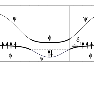
FIG. 1.: Illustration of the effective model and the FM mechanism. $\Delta$ is the hibridization gap and $\delta_{a}$ is the interval of energy where the electrons are polarized.

III New Mechanism for Ferromagnetism

The PAM has different regimes depending on the values of its parameters and the particle concentration $n=N_{e}/4N$ ($N_{e}$ is the total number of particles and $N$ is the number of unit cells). If $V\ll|\epsilon_{a}|$ and $V\ll|U+\epsilon_{a}|$, there is one particle (magnetic moment) localized in each $a$ orbital, and the fluctuations to the conduction band can be considered in a perturbative way. By this procedure, the PAM can be reduced to the Kondo Lattice Model (KLM) [44] which contains only one parameter $J_{K}/t$ (with $J_{K}=$ and $t=t_{b}$). The KLM has been extensively studied [45, 46, 47, 50], and the evolution of its phase diagram is described for instance in a review article by Tsunetsugu et al [48]. One of the earliest approaches to the KLM is the mean field treatment of Doniach [45] for the related one dimensional Kondo necklace. For half filling, this approximation leads to a transition from a Néel ordered state in the weak coupling regime ($J_{K}\ll|t|$) to a nonmagnetic ‘Kondo singlet’ state above the critical value $J_{K}^{c}=t$.

Lacroix and Cyrot [49] did a more extensive mean field treatment for three dimensional KLM. They also found a magnetically ordered state for weak coupling. For low density of conduction electrons. In their phase diagram, the ordered state is ferromagnetic for low and intermediate densities of conduction electrons, and antiferromagnetic in the vicinity of half filling. The ‘Kondo singlet’ phase appears above some critical value of $J_{K}^{c}(n)$ in the whole range of concentrations.

Using another mean field treatment for the one dimensional KLM, Fazekas and Müller-Hartmann [50] obtained a phase diagram containing only magnetically ordered phases: spiral below some critical value of $J_{K}/t$ which depends on the particle density and ferromagnetic above this value. To get this result, they fixed the orientation of the localized spins in a spiral ordering and minimized the total energy with respect to the wave vector of the spiral. Even though this treatment of the spin polarized state is valid for classical spins, it neglects completely the Kondo singlet formation which occurs in the strong coupling limit for the considered case ($S=1/2$).

Sigrist et al [51] gave an exact treatment of one dimensional KLM for the strong coupling regime $J_{K}\gg t$ finding a ferromagnetic phase for any particle density. However, it is important to remark that the mechanism driving the ferromagnetism in the later case is not the same as the double-exchange mechanism associated with the mean field solution of Fazekas and Müller-Hartmann [50]. To understand this difference, we just need to notice that for $J_{K}/t=\infty$ mean field [50] predicts a ferromagnetic solution while the exact solution has a complete spin degeneracy. Therefore double-exchange is not the mechanism driving the ferromagnetic phase of the KLM (at least when the localized spins are $S=1/2$).

The real mechanism has been unveiled by Sigrist et al [51] who used degenerate perturbation theory to determine the lifting of this degeneracy when the ratio $J_{K}/t$ becomes finite. The new ground state is an itinerant ferromagnet for any concentration of conduction electrons. In this state, the spins which are not participating in Kondo singlet are fully polarized. We can see from their solution that the motion of the Kondo singlets stabilizes the FM state in a way similar to Nagaoka’s solution [20]. The second order effective Hamiltonian obtained after the perturbative calculation includes nearest-neighbor hopping $t/2$, plus a next-nearest-neighbor correlated hopping $t^{\prime}$ which is order $t^{2}/J_{K}$. Then there are two different ways to move a Kondo singlet from one site to its next-nearest-neighbor: by two applications of $t/2$ or by one application of $t^{\prime}$. Only when the background is ferromagnetic do both processes lead to the same final state. If $t^{\prime}$ has the appropriate sign (which is the case for the KLM [51]) the resulting interference is “constructive” and the FM state has the lowest energy. We can see in this example that the motion of the Kondo singlet can stabilize a magnetic phase.

There are different regimes for which the PAM cannot be reduced to a KLM by a perturbative approach. One of these situations corresponds to the intermediate valence region: $\epsilon_{a}\sim E_{F}$. In this case $n^{a}_{i}$ is not longer close to one and the $a$ electrons can move.

In Fig. 1, we illustrate the (one-dimensional) non-interacting bands for the case of interest: $\epsilon_{a}$ close to $E_{F}$ and above the bottom of the $b$ band. If $|V|\ll|t_{b}|$, we can identify two subspaces in each band where the states have either $b$ ($\psi$ subspace) or $a$ ($\phi$ subspace) character. The size of the crossover region around the points where the original unhybridized $b$ and $a$ bands crossed is proportional to $|V/t_{b}|$; that is, it is very small. The creation operators for the Wannier orbitals $\psi^{\;}_{{\bf r}\sigma}$ and $\phi^{\;}_{{\bf r}\sigma}$ associated with each subspace are:

$$\psi^{\dagger}_{{\bf r}\sigma} = \frac{1}{\sqrt{N}}\Biggl{[}\sum_{{\bf k}\in{\bf K}^{>}}e^{i{\bf k\cdot r}}\beta^{\dagger}_{{\bf k}\sigma}+\sum_{{\bf k}\in{\bf K}^{<}}e^{i{\bf k\cdot r}}\alpha^{\dagger}_{{\bf k}\sigma}\Biggr{]}$$ (14)

$$\phi^{\dagger}_{{\bf r}\sigma} = \frac{1}{\sqrt{N}}\Biggl{[}\sum_{{\bf k}\in{\bf K}^{>}}e^{i{\bf k\cdot r}}\alpha^{\dagger}_{{\bf k}\sigma}+\sum_{{\bf k}\in{\bf K}^{<}}e^{i{\bf k\cdot r}}\beta^{\dagger}_{{\bf k}\sigma}\Biggr{]}.$$ (15)

where $N$ is the number of sites. The subsets ${\bf K}^{>}$ and ${\bf K}^{<}$ are defined by: ${\bf K}^{>}=\{{\bf k}:|u_{\bf k}|\geq|v_{\bf k}|\}$ and ${\bf K}^{<}=\{{\bf k}:|v_{\bf k}|>|u_{\bf k}\}$. Since the $\psi$ and the $\phi$ subspaces are generated by eigenstates of $H_{0}$, it is clear that both subspaces can only be mixed by the interacting term $H_{U}$. Therefore in the new basis we have:

$$H_{0}=H^{\phi}_{0}+H^{\psi}_{0}=\sum_{{\bf r,r^{\prime}},\sigma}\tau^{\phi}_{{\bf r-r^{\prime}}}\phi^{\dagger}_{{\bf r}\sigma}\phi^{\;}_{{\bf r^{\prime}}\sigma}+\sum_{{\bf r,r^{\prime}},\sigma}\tau^{\psi}_{{\bf r-r^{\prime}}}\psi^{\dagger}_{{\bf r}\sigma}\psi^{\;}_{{\bf r^{\prime}}\sigma},$$ (16)

with the hoppings $\tau^{\phi}_{{\bf r}}$ and $\tau^{\psi}_{{\bf r}}$ given by the following expressions:

$$\tau^{\phi}_{{\bf r}}=\frac{1}{N}\Biggl{[}\sum_{{\bf k}\in{\bf K}^{>}}e^{i{\bf k\cdot r}}E_{{\bf k}}^{-}+\sum_{{\bf k}\in{\bf K}^{<}}e^{i{\bf k\cdot r}}E_{{\bf k}}^{+}\Biggl{]}$$ (17)

$$\tau^{\psi}_{{\bf r}}=\frac{1}{N}\Biggl{[}\sum_{{\bf k}\in{\bf K}^{>}}e^{i{\bf k\cdot r}}E_{{\bf k}}^{+}+\sum_{{\bf k}\in{\bf K}^{<}}e^{i{\bf k\cdot r}}E_{{\bf k}}^{-}\Biggl{]}.$$ (18)

The segmented structure of the $\psi$ and the $\phi$ bands introduce oscillations in the hoppings $\tau^{\psi}_{{\bf r}}$ and $\tau^{\phi}_{{\bf r}}$ as a function of the distance $|{\bf r}|$.

Because the $U$ term in $H$ involves only the $a$ orbitals, the matrix elements of $H$ connecting the $\phi$ and $\psi$ subspaces are small compared to the characteristic energy scales of the problem (the matrix elements of $H$ within the subspaces). To see this we express $a_{{\bf r}\sigma}^{\dagger}$ as a function of $\phi^{\dagger}_{{\bf r}\sigma}$ and $\psi^{\dagger}_{{\bf r}\sigma}$ by first inverting Eqs. 13 and 15 to find:

$$a_{{\bf r}\sigma}^{\dagger}=\sum_{\bf r^{\prime}}W_{\bf r-r^{\prime}}\phi^{\dagger}_{{\bf r^{\prime}}\sigma}+w_{\bf r-r^{\prime}}\psi^{\dagger}_{{\bf r^{\prime}}\sigma},$$ (19)

where the weights $W_{{\bf r}}$ and $w_{{\bf r}}$ are defined by:

$$W_{{\bf r}}=\frac{1}{N}\Biggl{[}\sum_{{\bf k}\in{\bf K}^{>}}e^{i{\bf k\cdot r}}u_{\bf k}+\sum_{{\bf k}\in{\bf K}^{<}}e^{i{\bf k\cdot r}}v_{\bf k}\Biggr{]}$$ (20)

$$w_{{\bf r}}=\frac{1}{N}\Biggl{[}\sum_{{\bf k}\in{\bf K}^{>}}e^{i{\bf k\cdot r}}v_{\bf k}+\sum_{{\bf k}\in{\bf K}^{<}}e^{i{\bf k\cdot r}}u_{\bf k}\Biggr{]}.$$ (21)

The value of these weights as a function of the distance ${\bf r}$ is plotted in Fig. 2 (for $\epsilon_{a}=-1.5$, $V=0.1t$ and $t_{a}=0$). From Fig. 2 we can see that $W_{{\bf 0}}$ is much larger than any other weight. This is so because the $\phi$ orbitals have predominantly $a$ character, while the $\psi$ orbitals have mostly $b$ character in the considered region of parameters. Therefore we can approximate the creation operator $a_{{\bf r}\sigma}^{\dagger}$ by:

$$a_{{\bf r}\sigma}^{\dagger}\approx\sum_{\bf r^{\prime}}W_{\bf r-r^{\prime}}\phi^{\dagger}_{{\bf r}\sigma}$$ (22)

As a consequence of this approximation, the $a$ subspace becomes invariant under the application of $H$. In addition, because $|W^{\;}_{\bf 0}|\gg|W^{\;}_{\bf r\neq 0}|$ (see Fig. 2), we can establish a hierarchy of terms where the lowest order one corresponds to a simple on-site repulsion:

$$H^{U}_{eff}={\tilde{U}}\sum_{\bf r}n^{\phi}_{{\bf r}\uparrow}n^{\phi}_{{\bf r}\downarrow}$$ (23)

with $\tilde{U}=U|W_{\bf 0}|^{4}$ and $n^{\phi}_{{\bf r}\sigma}=\phi^{\dagger}_{{\bf r},\sigma}\phi^{\;}_{{\bf r},\sigma}$. The next order terms, containing three and two $W_{\bf 0}$ factors, are much smaller and are essentially the same as the intersite interactions which in the past were added to the Hubbard model to enhance the ferromagnetism [23].

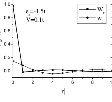
FIG. 2.: Weights $W_{\bf r}$ and $w_{\bf r}$ as a function of the distance $|{\bf r}|$ for a one dimensional system.

Adding $H^{U}_{eff}$ to $H_{0}$ we get the effective Hamiltonian:

$$H_{eff} = \sum_{{\bf r,r^{\prime}},\sigma}(\tau^{\psi}_{{\bf r-r^{\prime}}}\psi^{\dagger}_{{\bf r}\sigma}\psi^{\;}_{{\bf r^{\prime}}\sigma}+\tau^{\phi}_{{\bf r-r^{\prime}}}\phi^{\dagger}_{{\bf r}\sigma}\phi^{\;}_{{\bf r^{\prime}}\sigma})$$ (24)

$$+ {\tilde{U}}\sum_{\bf r}n^{\phi}_{{\bf r}\uparrow}n^{\phi}_{{\bf r}\downarrow}$$ (25)

The $\psi$ and $\phi$ orbitals form uncorrelated and correlated non-hybridized bands: $H_{eff}=H^{\psi}+H^{\phi}$. For the $\phi$ orbitals we obtain an effective one band Hubbard model with the peculiar double shell like dispersion relation shown by the thick lines in Fig. 1.

Particularly for $t_{a}=0$, $H^{\phi}$ has a very large density of states in the lower shell of the $\phi$ band [23] which is located near $\epsilon_{a}$ . From Fig. 1 it is also clear that the electrons first doubly occupy the uncorrelated $\psi$ band states which are below $\epsilon_{a}$. However, when $E_{F}$ gets close to $\epsilon_{a}$, i.e., the system is in the mixed valence regime, the electrons close to the Fermi level go into some of the correlated $\phi$ states. Then, the interaction term $H^{U}_{eff}$, combined with the double shell band structure of $H^{\phi}_{0}$, gives rise to a FM ground state (GS): The electrons close to $E_{F}$ spread to higher unoccupied ${\bf k}$ states and polarize, which causes the spatial part of their wave function to become antisymmetric, eliminating double occupancy in real space and reducing the Coulomb repulsion to zero. The cost of polarizing is just an increase in the kinetic energy proportional to $\delta_{a}\sim\hbar v_{F}\delta_{k}$, where $v_{F}$ is the Fermi velocity and $\delta_{k}$ is the interval in ${\bf k}$ space in which the electrons are polarized.

To determine the stability of this unsaturated FM state, we compare its energy with that of the PM state. If we were to build a nonmagnetic state with only the states of the lower $\phi$ shell, we would find a restricted delocalization for each electron because of the exclusion of the finite set of band states (${\bf k}$-states) in the upper shell. To avoid the Coulomb repulsion $U$ for double occupying a given site, the electrons need to occupy all ${\bf k}$-states. This means they have to occupy the $\phi$ states in the upper and lower shells. This restricted delocalization is a direct consequence of Heisenberg’s uncertainty principle, and the resulting localization length depends on the wave vectors, where the original $b$ and $a$ bands crossed, that define the size ($\Delta{\bf k}$) of each shell. The energy cost for occupying the $\phi$ states in the upper shell is proportional to the hybridization gap $\Delta$. Therefore if $U$ is the dominant energy scale in the problem and $\Delta\gg\delta_{a}$, the FM state lies lower in energy than the nonmagnetic state. Under these conditions, the effective FM interaction is proportional to the hybridization gap $\Delta$.

This mechanism for ferromagnetism on a lattice is analogous to the intra-atomic Hund’s mechanism polarizing electrons in atoms. In atoms, we also have different degenerate (the equivalent of $\delta_{a}$ is zero) shells separated by an energy gap. If the valence shell is open, the electrons polarize to avoid the short range part of the Coulomb repulsion (again reflecting the Pauli exclusion principle). The energy of an eventual nonmagnetic state is proportional either to the magnitude of the Coulomb repulsion or to the energy gap between different shells. The interplay between both energies sets the scale of Hund’s intra-atomic exchange coupling.

IV Numerical Method

Our numerical method, the constrained-path Monte Carlo (CPMC) method, is extensively described and benchmarked elsewhere.[57, 58] Here we only discuss its basic features, assumptions and special details about our use of it.

In the CPMC method, the ground-state wave function $|\Psi_{0}\rangle$ is projected from a known initial wave function $|\Psi_{T}\rangle$ by a branching random walk in an over-complete space of Slater determinants $|\phi\rangle$. In such a space, we can write $|\Psi_{0}\rangle=\sum_{\phi}c_{\phi}|\phi\rangle$, where $c_{\phi}>0$. The random walk produces an ensemble of $|\phi\rangle$, called random walkers, which represent $|\Psi_{0}\rangle$ in the sense that their distribution is a Monte Carlo sampling of $c_{\phi}/\sum_{\phi}c_{\phi}$, that is, a sampling of the ground-state wave function.

To completely specify $|\Psi_{0}\rangle$, only determinants satisfying $\langle\Psi_{0}|\phi\rangle>0$ are needed because $|\Psi_{0}\rangle$ resides in either of two degenerate halves of the Slater determinant space, separated by a nodal plane. In the CPMC method the fermion sign problem occurs because walkers can cross this plane as their orbitals evolve continuously in the random walk. Without a priori knowledge of this plane, we use a trial wave function $|\Psi_{T}\rangle$ and require $\langle\Psi_{T}|\phi\rangle>0$. The random walk solves Schrödinger’s equation in determinant space, but under an approximate boundary-condition. This is what is called the constrained-path approximation.

The quality of the calculation depends on the quality of the trial wave function $|\Psi_{T}\rangle$. Fortunately, extensive testing has demonstrated a significant insensitivity of the results to reasonable choices: Since the constraint only involves the overall sign of its overlap with any determinant $|\phi\rangle$, some insensitivity of the results to $|\Psi_{T}\rangle$ is expected [29, 57, 58, 59, 60, 61].

Besides as starting point and as a condition constraining a random walker, we also use $|\Psi_{T}\rangle$ as an importance function. Specifically, we use $\langle\Psi_{T}|\phi\rangle$ to bias the random walk into those parts of Slater determinant space that have a large overlap with the trial state. For all three uses of $|\Psi_{T}\rangle$, it clearly is advantageous to have $|\Psi_{T}\rangle$ approximate $|\Psi_{0}\rangle$ as closely as possible. Only in the constraining of the path does $|\Psi_{T}\rangle\not=|\Psi_{0}\rangle$ in general generate an approximation.

We constructed $|\psi_{T}\rangle=\prod_{\sigma}|\phi_{T}^{\sigma}\rangle$ from the eigenstates of the non-interacting problem. Because the total and z-component spin angular momentum, $S$ and $S_{z}$, are good quantum numbers, we could choose unequal numbers of up and down electrons to produce trial states and hence ground states with $S=S_{z}=\frac{1}{2}(N_{\uparrow}-N_{\downarrow})$. Whenever possible, we would simulate closed shells of up and down electrons, as such cases usually provided energy estimates with the least statistical error, but because we wanted to study the ground state energy as a function of $S$, we frequently had to settle for just the up or down shell being closed. In some cases, the desired value of $S$ could not be generated from either shell being closed. Also we would select the non-interacting states so $|\psi_{T}\rangle$ would be translationally invariant, even if these states used did not all come from the Fermi sea. The use of unrestricted Hartree-Fock eigenstates to generate$|\phi_{T}^{\sigma}\rangle$ instead of the non-interacting eigenstates generally produced no significant improvement in the results.

In particular, we represented the trial wavefunction as a single Slater determinant whose columns are the $N_{\sigma}$ single-particle orbitals obtained from the exact solution of $H_{0}$. We chose the orbitals with lowest energies given by $E^{-}_{\bf k}$ and filled them up to a desired number of electrons $N_{e}$.

$$|\psi_{T}\rangle=\prod_{\bf k,\sigma}\alpha_{{\bf k},\sigma}^{\dagger}|0\rangle,$$ (26)

where $|0\rangle$ represents a vacuum for electrons. Since our calculations were performed for a less than full lower band, only states from the lower band were used to construct the trial wavefunction.

In a typical run we set the average number of random walkers to 400. We performed 2000 Monte Carlo sweeps before we taking measurements, and we made the measurements in 40 blocks of 400 steps. By choosing $\Delta\tau=0.05$, we reduced the systematic error associated with the Trotter approximation to be smaller than the statistical error. In measuring correlation functions, we performed between 20 to 40 back-propagation steps.

V Quantum Monte Carlo Results

In section III, we have described a new mechanism for itinerant ferromagnetism which is present in the mixed valence regime for $n>~{}1/4$. In addition, we mentioned that the system is also expected to be FM when the $f$ magnetic moments are localized ($|V|\ll|E_{F}-\epsilon_{a}|$) because the effective RKKY coupling is negative when the Fermi surface is small ($k_{F}\sim 0$). In this section we show that the itinerant and the localized ferromagnetic states are continuously connected in the phase diagram of the PAM. However, the energy scale of the first state is much larger than the RKKY interaction which characterizes the second one. The existence of a crossover region between both states could explain the fact that there are some $f$-electron compounds for which it is very difficult to determine whether they are itinerant or localized ferromagnets.

In addition, we will see that the QMC results are consistent with the simple picture derived from our effective model (Eq. [25]). According to that picture, the ferromagnetic state in the mixed valence regime should be similar to a partially polarized non-interacting solution where the polarized electrons are the ones occupying the $f$-character orbitals. It is only in the crossover region of size $V^{2}/t_{b}$ (see Fig. 1), where the orbitals have a mixed character, that the correlations introduce an appreciable effect. This effect is the well known Kondo-like singlet correlation between the $d$ and the $f$ electrons. However, it is important to remark that these Kondo singlets only exist in an energy interval $V^{2}/W$ (where $W$ is the $d$ bandwidth), and therefore the number of Kondo singlets $N_{KS}$ is much smaller than the number of magnetic moments $N_{MM}$: $N_{KS}/N_{MM}\sim V^{2}/W^{2}$. This is a simple manifestation of the “exhaustion” phenomenon described by Nozierés [62, 63]. Since most of the $f$ magnetic moments are ferromagnetically polarized, the role of these few Kondo singlets is marginal in our FM solution. Therefore, for the mixed valence regime with $n>~{}1/4$, the $f$ magnetic moments which are not screened by $d$ electrons develop an effective magnetic interaction as a consequence of the interplay between the local Coulomb interaction and the particular band structure. In other words, the “collective Kondo state” which was proposed in the past [62, 63] is replaced by band ferromagnetism [28].

In fact, the nature of local moment compensation in the PAM differs qualitatively from that in the single impurity Anderson model [29]. In the PAM, if the ground state is a singlet, then

$$\langle S^{z}_{f}(j)^{2}\rangle=-\sum_{i}\langle S^{z}_{d}(i)S^{z}_{f}(j)\rangle-\sum_{i}\langle S^{z}_{f}(i)S^{z}_{f}(j)\rangle$$ (27)

In the impurity model, the last term is absent, and the resulting expression is the analytic statement of the well-known Clogston-Anderson compensation theorem that express the compensation of the f-moment by the conduction electrons. In the PAM, on the other hand, the last term dominates the first so the f-moment is compensated largely by correlations induced among themselves.

To understand the nature of the FM solution, we plotted the mean occupation number of the quasiparticle operators which diagonalize the non-interacting problem (see Eq. 11). This is shown in Fig. 3 for the lowest energy PM ($S=0$) state in a two dimensional cluster of $12\times 12$ unit cells. There we can see that the $d$-character states of the lower band are close to be doubly occupied. In contrast, the $f$-character region has a smaller occupation number ($\sim 0.7$). It is remarkable that the populations of the $f$-character states in the lower and the upper bands are very similar. This delocalization in the momentum space is a direct consequence of the tendency to avoid double-occupancy in the real space. This tendency indicates that the energy increase of the PM state due to the inclusion of $U$ is proportional to the hybridization gap.

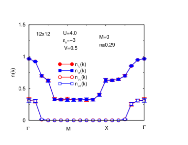
FIG. 3.: Mean value of the occupation numbers of the non-interacting band states for the paramagnetic $S=0$ solution of the PAM in a two dimensional lattice. Legends: $n_{lu}({\bf k})$ represents lower-band occupation number of up-spins, $n_{ud}({\bf k})$ represents upper-band occupation number of down-spins, etc.

Fig. 4 shows the quasiparticle occupation numbers for the partially saturated FM ground state. While the $b$-character states of the lower band are still close to being doubly occupied, the $a$-character ones are polarized and the occupation number is one for any of them. In contrast to the PM solution (see Fig.3), the occupation number for the $f$-character states in the upper band is much smaller. This difference can be understood in the following way: the polarized $f$-electrons can localize in momentum space because the Pauli exclusion principle prevents double occupancy in real space (the spatial wave function is completely antisymmetric). Therefore the $a$-electrons do not need to occupy the upper band states and the energy increase due to the repulsive $U$ term is proportional to $\hbar v_{F}\delta_{k}$. The non-zero amount of electrons occupying the center of the upper band (see Fig. 4) is related to the crossover region for which the $a$ and the $b$ character of the states are comparable. Since the electrons occupying these states are not polarized, the effect of the Coulomb repulsion $U$ is the transfer of spectral weight from the lower to the upper band to avoid double occupancy in real space.

We can see from Figs. 5 and 6 that a similar behavior is obtained for one dimensional systems. As we explained in section III, the mechanism for this ferromagnetism works in any finite dimension. Notice in Fig. 5 that there is a jump in the occupation number of the lower band as a function of ${\bf k}$. The inverse of this jump is proportional to effective mass of the quasiparticles of the pramagnetic solution. When $\epsilon_{a}$ decreases, the system evolves into a state where the $a$ electrons are localized. This evolution is reflected in the decrease of the jump and the consequent increase of the effective mass.

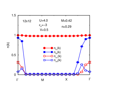
FIG. 4.: Mean value of the occupation numbers of the non-interacting band states for the ground state (partially saturated ferromagnet with $M=S/N=0.43$) of the PAM in a two dimensional lattice.

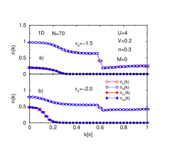
FIG. 5.: Mean value of the occupation numbers of the non-interacting band states for the paramagnetic $S=0$ solution of the PAM in a chain.

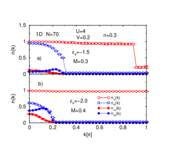
FIG. 6.: Mean value of the occupation numbers of the non-interacting band states for the ground state (partially saturated ferromagnet with $M=S/N=0.3$) of the PAM in a chain.

For $U=0$ the system is a PM metal. Therefore there must be a critical value of the on site repulsion $U_{c}$ which separates the PM from the FM region. The value obtained for $U_{c}$ is: $U_{c}\sim 0.25\sim\Delta=0.242$ for $V=0.5$ and $U_{c}\sim 0.11\sim\Delta=0.0981$ for $V=0.31$ (see Fig. 7). This is also in agreement with the mechanism described in section III. If $\Delta\gg\delta$ and $U$ becomes larger than the hybridization gap $\Delta$, the system evolves into a FM state to avoid the double occupancy without an increase in the kinetic energy proportional to the hybridization gap.

According to Figs. 7b and 8 the magnetization seems to increase gradually when $U$ is increased beyond its critical value. This behavior suggests that the FM transition as function of $U$ is of second order. If this is so, the properties of the PM Fermi liquid which is obtained for $U<U_{c}$ should be strongly affected by the FM fluctuations when $U$ approaches $U_{c}$. It is known that the effective mass of the quasi-particles diverges in the approach to a zero temperature ferromagnetic instability [52, 53, 54, 55]. In other words, the behavior of the PM Fermi liquid cannot be understood by analogy with the one impurity problem. The Kondo temperature, which is the characteristic energy scale of the one impurity problem, is replaced by a new Fermi temperature which is dominated by the ferromagnetic fluctuations and goes to zero when $U$ approaches to $U_{c}$ from below.

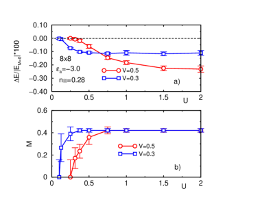
FIG. 7.: a) Energy difference between partially polarized FM ground state and the lowest energy paramagnetic state as a function of $U$. b) Magnetization as a function of $U$.

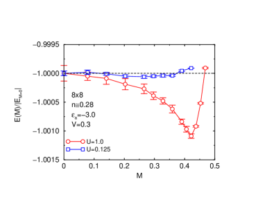
FIG. 8.: Minimum energy as a function of the magnetization.

Another relevant parameter for the FM solution is the hybridization $V$. For $V=0$ and $\epsilon_{a}=E_{F}$ there is a complete spin degeneracy for the electrons occupying the localized $a$ orbitals. By increasing $V$, we are simultaneously changing the Fermi velocity $v_{F}$ and the hybridization gap $\Delta$. For small values of $V$, $\Delta$ is much larger than $\delta=\hbar v_{F}\delta_{k}$ in the region under consideration. For this reason, a non-zero value of $V$ removes the original spin degeneracy stabilizing the partially polarized FM solution (see Fig. 9). When $V$ is larger than $t$, the two relevant energy scales, $\Delta$ and $\delta$, become of the same order and the partially polarized FM is replaced by a PM phase. In the unrealistic large $V$ limit ($|V|\gg|t_{b}|,U,|\epsilon_{a}|$), the ground state consists of local Kondo singlets moving in a background of localized spins [56].

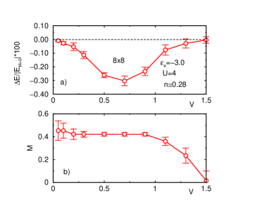
FIG. 9.: a) Energy difference between the FM ground state and the lowest energy paramagnetic state as a function of $V$. b) Magnetization as a function of $V$.

Finally, the most sensitive parameter for the stabilization of the FM state is the difference $|\epsilon_{a}-E_{F}|$. In Fig. 10, we show the energy difference $|\Delta E|$ between the FM ground state and the lowest energy PM ($S=0$) state as a function of $\epsilon_{a}$. When $\epsilon_{a}$ is considerably smaller than $E_{F}$, the $a$ electrons are localized and the magnetism is dominated by the RKKY interaction. The order of this interaction is $V^{4}$. This gives the small value of $|\Delta E|$ when the $a$ levels are below the bottom of the conduction band $\epsilon_{a}<-2D|t_{b}|$. The most stable region for the FM state (maximum value of $|\Delta E|$) starts when $\epsilon_{a}$ reaches the Fermi level. For the case of Fig. 10, this occurs at $\epsilon_{a}\sim-1.9t$. Again this result is in agreement with the mechanism described in section III. If we continue increasing the value of $\epsilon_{a}$, the number of $a$ electrons decreases and the magnetization is consequently reduced (see Fig. 10b). Finally, when $\epsilon_{a}$ is no longer close to the bottom of the conduction band, $\delta_{a}$ becomes comparable to $\Delta$ and the ferromagnetism disappears.

Fig. 11 shows the $\epsilon_{a}$ dependence of $|\Delta E|$ for two and three dimensional clusters. As in the one dimensional case, the stablity of the FM phase increases when the system appraches the mixed valence regime. If $\epsilon_{a}$ is further increased, the magnetization goes to zero in a smooth way indicating that the associated quantum phase transition is of second order.

In Figs. 12 and 13 we show the scaling of $\Delta E$ and the magnetization per site in one and two dimensional systems. The $1/N$ extrapolation for the one dimensional systems indicates that the FM ground state is stable in the thermodynamic limit. The extrapolated value for the magnetization is $\sim 0.3$, i.e., only a fraction of the $f$ electrons is polarized. The size effects are stronger in two dimensional systems. In Fig. 13, we show two different cases: the circles correspond to a sequence of tilted suqare clusters which allows us to fix the concentration in $n=0.3$; the squares correspond to a sequence of untilted square clusters for which the value of the concentration is the closest to $n=0.29$. Despite the considerable size effects, these results indicate that the FM state is stable in the thermodynamic limit. In this case, the extrapolated magnetization is close to 0.4.

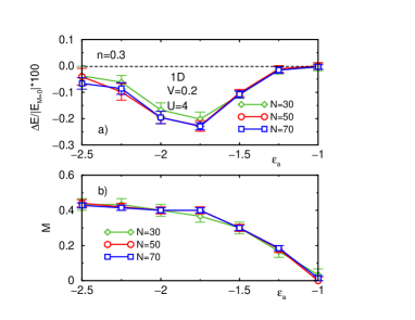
FIG. 10.: a) Energy difference between FM ground state and the lowest energy paramagnetic state as a function of $\epsilon_{a}$ for a one dimensional system. b) Magnetization as a function of $\epsilon_{a}$.

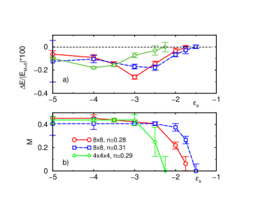
FIG. 11.: a) Energy difference between FM ground state and the lowest energy paramagnetic state as a function of $\epsilon_{a}$ for two and three dimensional systems. b) Magnetization as a function of $\epsilon_{a}$.

Meyer and Nolting [39] have also found a FM solution for the PAM in a similar region of parameters using DMFT. However it is important to remark that the mechanism for ferromagnetism described in section III only works in finite dimension because the volume of the upper shell relative to the volume of the lower one goes to zero when the dimension goes to infinity. Therefore, the reason why a FM state is obtained with DMFT should be different. This is also reflected by the fact that the energy scale ($T_{c}$) of the FM solution found with DMFT for the localized regime is larger than the one for the mixed valence regime (region IV of Ref. [37]). This behavior is opposite to our result (see Fig. 10).

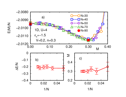
FIG. 12.: a) Scaling of the energy difference between the FM ground state and the lowest energy paramagnetic state for different chain lengths. b) Scaling of the magnetization per site.

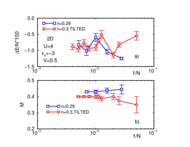
FIG. 13.: a) Scaling of the energy difference between the FM ground state and the lowest energy paramagnetic state for two dimensional systems. b) Scaling of the magnetization per site.

VI Experimental Consequences

A Cerium Compounds

During the last few years new experimental results have confirmed that there are Ce based compounds which cannot be treated as typical Kondo systems. For instance, CeRh₃B₂ has a very high FM ordering temperature ($T_{c}=115^{\circ}K$) which sicks out from a localized $4f$-electron description [42]. In addition the alloy series Ce(Rh_1-xRu_x)₃B₂ [42] and La_xCe_1-xRh₃B₂ [64] exhibit many unusual characteristics which require a new macroscopic description with respect to the competition among classical Kondo versus RKKY interactions [45].

Absorption edge spectroscopy measurements of Ce(Rh_1-xRu_x)₃B₂ for different values of $x$ indicate that the stoichiometric compound CeRh₃B₂ is in the mixed valence regime (fluctuating between the $4f^{1}$ and the $4f^{0}$ configurations) [42]. After doping with Ru, there is strong transfer of weight from the $4f^{1}$ line to the $4f^{0}$ structure. This change can be understood in the context of the PAM if we take into account that the volume of the system decreases when Ce is replaced by Rh [64]. In this situation the width of the conduction band increases and some $f$ electrons are transferred to $d$ character orbitals (see Fig.1). According to our results this change must decrease the value of the zero temperature magnetization and the Curie temperature $T_{c}$. By increasing the doping level we can reach a situation where most of the $f$ electrons that were polarized in the stoichiometric compound are transferred to the $d$ character orbitals and the zero temperature magnetization is very small. In this limit the system should have some PM states very close to the Fermi level (see Fig. 1). When the energy difference between the Fermi level and these PM states becomes smaller than $T_{c}$, the magnetization can increase with temperature because the electrons which are occupying the PM states near the Fermi level are thermally promoted to the $f$ character states which are above the Fermi level. In this process, the electrons are polarized because of the mechanism discussed above. This explains the finite temperature peak in the magnetization of Ce(Rh_1-xRu_x)₃B₂ (for $x$ between 0.06 and 0.125) [41, 42] that suggests an ordered state with high entropy. The source of the large entropy is thus associated with charge and not with spin degrees of freedom which is why a state with larger $M$ has a higher entropy. From this analysis we predict that the integral of the entropy below $T_{c}$, which can be extracted from the specific heat measurements, contains a considerable contribution from the the charge degrees of freedom.

When Ce is replaced by La, the volume of the system increases [64] and the magnetic moments become more localized. In this case, the weight in the absorption edge spectroscopy is transferred from the $4f^{0}$ structure to the $4f^{1}$ line. Again this can be understood if we take into account that the width of the conduction band decreases in this case and the electrons are transferred from the $d$ to the $f$ character orbitals (see 1). In this way the system evolves from the itinerant to the localized situation ($\epsilon_{f}=\epsilon_{a}<E_{F}$). According to our results (see Fig.10), this change should increase the value of the zero temperature magnetization and simultaneously decrease the Curie temperature $T_{c}$ ($|\Delta E|$ is strongly reduced because the effective magnetic interaction in the localized limit, $J_{RKKY}$, is order $V^{4}$ [1]). This anomalous behavior has been experimentally observed by Shaheen et al [64] in La_xCe_1-xRh₃B₂.

We can also connect our mechanism with the hydrostatic pressure dependence of $T_{c}$. To do this we calculated $|\Delta E|/N$ by the QMC method as function of increasing $t_{b}$ (Fig. 14a). Here we are assuming that the main effect of the hydrostatic pressure is to increase $t_{b}$ and to leave the other parameters unchanged. The order of magnitude of $|\Delta E|/N$, which should be proportional to $T_{c}$, and its qualitative behavior in Fig. 3a are in good agreement with the experimental results for CeRh₃B₂ [19]. We see from Fig. 3a that for the itinerant FM case, $|\Delta E|$/N is of the order of 100^∘K. This scale is much larger than the magnitude of the RKKY interaction [65] ($\sim 1^{\circ}$K) which is commonly used to explain the origin of the magnetic phase when the $a$ electrons are localized. We also find that the FM state appears close to quarter filling and disappears for $n$ close to $3/8$.

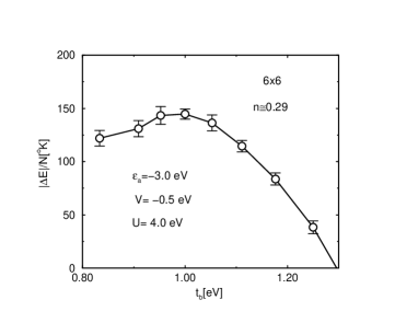
FIG. 14.: a) Energy difference per site between the FM and PM states as a function of $t_{b}$.

B Uranium Compounds

The FM uranium monochalcogenides US, USe and UTe are semi-metals with large Curie temperatures of $T_{c}=180K$, $160K$ and $108K$ and ordered moments of 1.5, 2.0 and 2.2$\mu_{B}$ respectively [24]. Most of the magnetic properties of these systems are still unexplained. The purpose of this subsection is to argue that the new mechanism for ferromagnetism introduced above is a good candidate to explain some of the mysteries related to these compounds.

Erdös and Robinson [66] suggested that the uranium monochalcogenides are mixed valence systems. This suggestion was reinforced by measuring the Poisson ratio as a function of the chalcogen mass with low temperature ultrasonic studies on USe and UTe [67]. The coexistence of an intermediate valence regime and ferromagnetism is one of the unexplained properties of these compounds as it is recognized in Ref. [24]. According to the traditional picture [45], the system should behave as a nonmagnetic collective Kondo state in the intermediate valence regime. In contrast to this picture, our results show that a partially saturated ferromagnetic state is stabilized in the mixed valence regime. This can explain the first striking property of the uranium monochalcogenides.

The other unusual property of these compounds is the shape of the magnetization curve versus temperature which has a maximum below $T_{c}$ [66]. Again this is a property which can be easily explained (see the subsection about the Ce compounds) within the context of the PAM. In addition, the order of magnitude of the Curie temperature of these compounds coincides with the energy scale obtained from the PAM for the intermediate valence regime.

The uranium monochalcogenides, like the Ce based compounds above described, exhibit a non-monotonic behavior for the $T_{c}$ as a function of pressure [19]. Fig. 14 shows that this behavior can also be explained with the PAM. Notice however that the non-monotonic behavior shown in Fig. 14 has nothing to do with a competition between Kondo and RKKY interactions.

Finally, the spin wave dispersions of these compounds also present some anomalies. For instance, neutron scattering experiments on a single-domain UTe crystal ([68, 69]) show that for wave vectors $q$ perpendicular to the ordered moment the excitations become more damped with increasing $q$. In US only a broad continuum of magnetic response is observed [70]. Damped and unpolarized spin waves are observed in USe [71, 72, 73]. These properties indicate that the itinerant character of the $f$ electrons is essential to have a good description of the magnetic excitations.

C Transition Metals

Even though the transition metals are the most well studied itinerant ferromagnets, the ultimate reason for the stabilization of the FM phase is still unknown. Since the minimal correlated model (Hubbard Hamiltonian) proposed to describe these systems does not seem to have a FM solution, it is reasonable to ask whether an extension of this minimal model, including more than one band, is necessary and enough to stabilize the FM solution. The correlated $3d$ band of the transition metals is hybridized with weakly correlated and dispersive $s$ and $p$ bands. This situation is similar to the case already described for the $f$ electron compounds. Therefore, it is natural to ask if there is a connection between the itinerant ferromagnetism of the $f$ and the $d$ electron compounds. Notice that the order of magnitude of the $T_{c}$ is the same. Following the same motivation and using DMFT, Schwieger and Nolting [43] concluded that the $d$-band ferromagnetism can be stabilized when the hybridization between both bands is small. However, these authors also find a FM solution for the one band problem.

In the case of the transition metals, the dispersion of the narrower band ($3d$) cannot be neglected. For this reason, we studied the stability of the FM solution as a function of $t_{a}$. We can see from Fig. 15 that the FM phase is even more stable for $t_{a}\sim-0.1$ than for $t_{a}=0$ and becomes unstable for $t_{a}\sim 0.05$. The reason for this asymmetric behavior is easy to understand in terms of the variation of $\delta_{a}$: If $t_{a}$ is negative, then the effect of $t_{a}$ on the dispersion of the $\phi$ band is opposite to that of the hybridization $V$ (see Fig. 16). When $t_{a}\sim-0.1$, we get, for the given $\epsilon_{a}$ and $V$, the minimum value for $\delta_{a}/\Delta$ and therefore the most stable FM case. When we depart from this value of $t_{a}$, $\delta_{a}/\Delta$ increases, $|\Delta E|$ decreases, and the FM state becomes less stable.

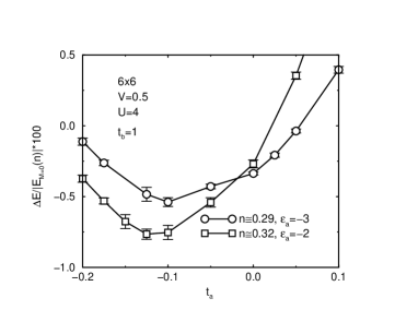
FIG. 15.: Influence of the hopping $t_{a}$ on the FM state.

This result indicates that the hybridization between bands can play a crucial role for the ferromagnetism of the iron group. In other words, the ferromagnetism of the transition metals can originate, at least in part, in the interplay between the correlations and the particular band structure and not solely in the intra-atomic Hund’s exchange [15].

FIG. 16.: Band structure for different values of $t_{a}$.

VII Conclusions

We introduced a novel mechanism for itinerant ferromagnetism which is present in a simple two band model consisting of a narrow correlated band hybridized with a dispersive and uncorrelated one. The picture just presented, combined with our previous results [1], allows a reconciliation of the localized and delocalized ferromagnetism pictures painted by Heisenberg [2] and Bloch [3]. The hybridization between bands and the particular band structure play a crucial role in this mechanism because they generate a multi-shell structure for the correlated orbitals. This structure, when combined with the a local Coulomb repulsion, favors a ferromagnetic state. The mechanism is analogous to the one which generates the atomic Hund interaction. In this sense, this is a generalization to the solid of the atomic Hund’s rule. The mechanism works in any finite dimension.

The determination of a minimal model to explain the metallic ferromagnetism of highly correlated systems has been the object of intense effort during the last forty years. The results presented in this paper suggest that the PAM is a minimal Hamiltonian which can explain the itinerant ferromagnetism without including any explicit FM interaction.

Another important aspect of this ferromagnetic solution is its mixed valence character. According to the traditional picture [45], the mixed valence regime should be a PM Kondo state. The appearance of a ferromagnetic instability in this region of doping rises some questions about the entire validity of a Kondo-like description inspired by the one impurity problem. Even the PM phase obtained for $U<U_{c}$ is strongly influenced by the proximity to a FM instability [52, 53, 54, 55].

We have discussed the relevance of these results for some $f$-electron compounds which are itinerant ferromagnets with high Curie temperatures ($\sim 100^{\circ}K$). In particular, the are several unusual characteristics of the Ce based compounds Ce(Rh_1-xRu_x)₃B₂ and La_xCe_1-xRh₃B₂, and the uranium monochalcogenides US, USe and UTe, which can be explained, at least at a qualitative level, with the present mechanism.

We have also considered the case relevant for the iron group where the dispersion of the lower band is not negligible. The fact that the ferromagnetism is even more stable for finite values of $t_{a}$ when the hoppings of both bands have opposite signs indicates that our mechanism is relevant to explain the ferromagnetism of the transition metals, like Ni, where a correlated and narrow $3d$ band is hybridized with the $4s$ band. It suggests that the ferromagnetism in the transition metals can originate, at least in part, in the interplay between the correlations and the particular band structure, and not solely in the intra-atomic Hund’s exchange [15].

- [1] C. D. Batista, J. Bonča and J. E. Gubernatis, Phys. Rev. Lett. 88, 187203 (2002).
- [2] W. Heisenberg, Z. Physik 49, 619 (1928).
- [3] F. Bloch, Z. Physik 57, 545 (1929).
- [4] E. P. Wigner, Phys. Rev. 46, 1002 (1934); E. P. Wigner, Trans. Faraday Soc. 34, 678 (1938).
- [5] J. C. Slater, Phys. Rev. 49, 537 (1936); J. C. Slater, Phys. Rev. 49, 931 (1936).
- [6] E.C. Stoner, Proc. Roy. Soc. (London) A165, 372 (1938). E.C. Stoner, Proc. Roy. Soc. (London) A169, 339 (1939).
- [7] J. H. van Vleck, Rev. Mod. Phys. 25, 220 (1953).
- [8] J. C. Slater, Phys. Rev. 49, 537 (1936).
- [9] M. C. Gutzwiler, Phys. Rev. Lett. 10, 59 (1963).
- [10] J. Hubbard, Proc. Roy. Soc. A 266, 238 (1963).
- [11] J. Kanamori, Prog. Theor. Phys. 30, 275 (1963).
- [12] E. P. Wohlfarth, Rev. Mod. Phys. 25, 211 (1953).
- [13] E.C. Stoner, Phys. Soc. Rept. Progress Phys. 11, 43 (1948); E.C. Stoner, J. Phys. et radium 12, 43 (1948)
- [14] J. C. Slater, Phys. Rev. 49, 537 (1936).
- [15] J. H. van Vleck, Rev. Mod. Phys. 25, 220 (1953).
- [16] M. C. Gutzwiler, Phys. Rev. Lett. 10, 59 (1963).
- [17] J. Hubbard, Proc. Roy. Soc. A 266, 238 (1963).
- [18] J. Kanamori, Prog. Theor. Phys. 30, 275 (1963).
- [19] A. L. Cornelius and J. S. Schilling, Phys. Rev. B 49, 3955 (1994).
- [20] Y. Nagaoka, Phys. Rev. 147, 392 (1966).
- [21] E. H. Lieb, Phys. Rev. Lett. 62, 1201 (1988).
- [22] E. H. Lieb and D. C. Mattis, Phys. Rev. 125, 164 (1962).
- [23] D. Vollhardt et al., Z. Phys. B 103, 287 (1997); D. Vollhardt et al., cond-mat/9804112 (to appear in Advances in Solid State Physics, Vol. 38).
- [24] P. Santini, R. Lémanski and P. Erdös, Advan. in Phys. 48, 537 (1999).
- [25] R. Hlubina, S. Sorella and F. Guinea, Phys. Rev. Lett. 78, 1343 (1997).
- [26] P. Fulde, J. Keller, and G. Zwicknagl, Solid State Physics, edited by H. Ehrenreich and D. Turnbull (Academic, New York, 1990), Vol. 41, p.1; H. R. Ott, in Progress in Low Temperature Physics, edited by D. F. Brewer (North-Holland, Amsterdam, 1987), Vol. XI, p. 215.
- [27] S. Daul and R. M. Noack, Phys. Rev. B 58, 2635 (1998).
- [28] P. Fazekas, Phil. Mag. B 76, 797 (1997).
- [29] J. Bonča and J. E. Gubernatis, Phys. Rev. B 58, 6992 (1998).
- [30] C. D. Batista, J. Bonča and J. E. Gubernatis, Phys. Rev. B, 63, 184428 (2001).
- [31] M. Guerrero and R. M. Noack, Phys. Rev. B 53, 3707 (1996).
- [32] M. Guerrero and R. M. Noack, cond-mat/0004265.
- [33] B. Möller and P. Wölfe, Phys. Rev. B 48, 10320 (1993).
- [34] Roman Doradziński and Jozef Spalek, Phys. Rev. B 56, 14239 (1997).
- [35] Roman Doradziński and Jozef Spalek, Phys. Rev. B 58, 3293 (1998).
- [36] A. N. Tahvildar-Zadeh, M. Jarrell, and J. K. Freericks, Phys. Rev. B 55, R3332 (1997).
- [37] D. Meyer, W. Nolting, G. G. Reddy, and A. Ramakanth, Phys. Stat. Sol. (b) 208, 473 (1998).
- [38] D. Meyer and W. Nolting, Phys. Rev. B 61, 13465 (2000).
- [39] D. Meyer and W. Nolting, Phys. Rev. B 62, 5657 (2000).
- [40] S. Schwieger and W. Nolting, cond-mat/0106638. 5657 (2000).
- [41] S. K. Malik, A. M. Umarji, G. K. Shenoy, and P. A. Montano, M. E. Reeves, Phys. Rev. B 31, 4728 (1985)
- [42] S. Berger, A. Galatanu, G. Hilscher, H. Michor, Ch. Paul, E. Bauer, P. Rogl, M. Gómez-Berisso, P. Pedrazzini, J. G. Sereni, J. P. Kappler, A. Rogalev, S. Matar, F. Weill, B. Chevalier, and J. Etourneau, Phys. Rev. B 64, 134404 (2001).
- [43] S. Schwieger and W. Nolting, Phys. Rev. B 64, 144415 (2001).
- [44] J. R. Schrieffer and P. A. Wolff, Phys. Rev. 149, 4910 (1996).
- [45] S. Doniach, Physica B 91, 231 (1977).
- [46] R. Jullien, P. Pfeuty, A. K. Bhattacharjee and B. Coqblin, J. App. Phys. 50, 7555 (1979).
- [47] P. Santini and J. Sólyom, Phys. Rev. B 46, 7422 (1996).
- [48] H. Tsunetsugu, M. Sigrist, and K. Ueda, Rev. Mod. Phys. 69, 809 (1997).
- [49] C. Lacroix, Solid State Comm. 54, 991 (1985).
- [50] P. Fazekas and E. Müller-Hartmann, Z. Phys. B 85, 285 (1991).
- [51] M. Sigrist, H. Tsunetsugu, K. Ueda, and T. M. Rice, Phys. Rev. B 46, 13838 (1992).
- [52] W. F. Brinkman and T. M. Rice, Phys. Rev. B 2, 4302 (1970).
- [53] D. Vollhardt, Rev. Mod. Phys. 56, 99 (1984).
- [54] M. T. Bal-Monod, Physica 109 110B, 1837 (1982).
- [55] T. Moriya and J. Kawabata, J. Phys. Soc. Japan 34, 639 (1973); J. Phys. Soc. Japan 35, 669 (1973).
- [56] C. D. Batista, J. Boncǎ and J. E. Gubernatis, preprint.
- [57] S. Zhang, J. Carlson and J. E. Gubernatis, Phys. Rev. Lett., 74, 3652 (1995).
- [58] S. Zhang, J. Carlson and J. E. Gubernatis, Phys. Rev. Lett., 74, 3652 (1995); Phys. Rev. B 55, 7464 (1997); J. Carlson, J. E. Gubernatis, G. Ortiz, and Shiwei Zhang, Phys. Rev. B 59, 12788 (1999).
- [59] M. Guerrero, J. E. Gubernatis, S. Zhang, Phys. Rev. B 57, 11980 (1998)
- [60] M. Guerrero, G. Ortiz, and J. E. Gubernatis, Phys. Rev. B 59, 1706 (1999)
- [61] M. Guerrero, G. Ortiz, and J. E. Gubernatis, Phys. Rev. B 62, 600 (2000).
- [62] P. Noziéres, Ann. Phys. (Paris) 10, 19 (1985).
- [63] P. Noziéres, Eur. Phys. J. B 6, 447 (1998).
- [64] S. A. Shaheen, J. S. Schilling, and R. N. Shelton, Phys. Rev. B 31, 656 (1985).
- [65] P.-G. de Gennes, Comm. Energie At. (France) Rappt. 925, (1959).
- [66] P. Erdd̈os and J. Robinson, The Physics of Actinide Compounds (New York, London:Plenum Press, 1983).
- [67] J. Neuenschwander, O. Vogt, E. Voit and P. Wachter, Physica B 144, 66 (1986).
- [68] G. H. Lander, W. G. Stirling, J. M. Rossat-Mignod, M. Hagen and O. Vogt, Physica B 156 157, 826 (1989).
- [69] G. H. Lander, W. G. Stirling, J. M. Rossat-Mignod, J. M. Hagen and O. Vogt, Phys. Rev. B 41, 6899 (1990).
- [70] W. J. L. Buyers and T. M. Holden. Neutron Scattering from Spins and Phonons in actinide systems, Handbook on the Physics and Chemistry of the Actinides, Vol. 2, edited by A. J. Freeman and G. H. Lander (New York: North-Holland, 1985).
- [71] P. de V. DuPlessis, J. Magn. Magn. Mater. 54-57, 537 (1986).
- [72] T. M. Holden, W. J. L. Buyers, P. de V. DuPlessis, K. M. Hughes and M. F. Collins, J. Magn. Magn. Mater. 54-57, 1175 (1986).
- [73] K. M. Hughes, T. M. Holden, W. J. L. Buyers, P. de V. DuPlessis and M. F. Collins, J. appl. Phys. 61, 3412 (1987).