Shot Noise and the Transmission of Dilute Laughlin Quasiparticles

Abstract

We analyze theoretically a three-terminal geometry in a fractional quantum Hall system - studied in a recent experiment - which allows a dilute beam of Laughlin quasiparticles to be prepared and subsequently scattered by a point contact. Employing a chiral Luttinger liquid description of the $\nu^{-1}=m$ integer edge states, we compute the current and noise of the quasiparticle beam after transmission through the point contact at finite temperature and bias voltage. A re-fermionization procedure at $m=2$ allows the current and noise to be computed non-perturbatively for arbitrary transparency of the point contact. Surprisingly, we find for weak backscattering the zero temperature limit is subtle and singular even at fixed finite bias voltage. In particular, at $T=0$ the incident charge $e/m$ quasiparticles are either reflected or else Andreev scattered (backscattering a charge $(-1+1/m)e$ quasihole and transmitting an electron) - Laughlin quasiparticles are not transmitted in this limit. A direct signature of these Andreev processes should be accessible in a particular cross-correlation noise measurement that we propose.

I Introduction

One of the most striking consequences of strong correlation in electronic systems is charge fractionalization, where the elementary charged excitations of a system have quantum numbers which differ from those of the bare electron. The fractional quantum Hall effect is an ideal arena to study this phenomena[1]. At filling factor $\nu=1/m$, the elementary excitation of the quantum Hall state is the charge $e/m$ Laughlin quasiparticle[2]. Current experimental techniques allow for a detailed study of the transport properties of these exotic particles.

A powerful technique for probing elementary charge carriers is to measure shot noise. When particles flow independently with an uncorrelated Poisson distribution, their charge is given by the ratio between the mean square fluctuation of the current and the average current[3]. In 1994 we proposed that a quantum point contact, formed by pinching together the edges of a quantum Hall bar, would be an ideal geometry for establishing the uncorrelated flow of Laughlin quasiparticles[4]. When the point contact is strongly pinched off the sample is effectively split into two. In that case a weak tunneling current must be carried by electrons, and shot noise with charge $e$ is expected. However, in the opposite extreme of weak pinch off, quasiparticles can backscatter between the edges through the quantum Hall fluid. The ratio between the noise and the backscattered current is then determined by the charge of the quasiparticle. In seminal 1997 experiments, de-Piccioto et al. [5] and Saminadayar, et al. [6] independently used this technique to measure the charge $e/3$ of the Laughlin quasiparticle.

The original experiments used a two terminal setup in which the current and noise transmitted through the point contact were measured. The backscattered current was determined by taking the difference between the measured current and the current at perfect transmission. Recently, Comforti et al.[7], have used the three terminal device consisting of two point contacts shown in Fig. 1. Consider first the case where the second point contact (QPC2) is completely open, while the first point contact (QPC1) is weakly pinched off. When voltage is applied to lead 1 with leads 2 and 3 grounded, quasiparticles backscattered from QPC1 propagate into lead 3. This geometry is superior to the two terminal setup for measuring the quasiparticle charge because the current due to the quasiparticles is isolated in lead 3. More interestingly, this may be viewed as a method for generating a dilute beam of Laughlin quasiparticles propagating into lead 3. This opens the door to experiments that probe the transport properties of and interactions between individual Laughlin quasiparticles.

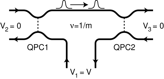
FIG. 1.: Schematic diagram of the three terminal fractional quantum Hall device with two quantum point contacts used by Comforti et al. A voltage $V$ is applied to lead 1 with leads 2 and 3 grounded. When the backscattering at QPC1 is weak, a dilute beam of Laughlin quasiparticles is directed along the top edge to QPC2.

Comforti et al. [7] used this technique to study a dilute beam of charge $e/3$ quasiparticles after transmission through the second point contact, QPC2. By measuring the current and noise in lead 3, they probed the average charge of the particles transmitted through QPC2. Surprisingly, they found that even when the transmission of QPC2 was small, of order $0.1$, the measured transmitted charge $\sim 0.45e$ was significantly smaller than that of the electron. This led them to suggest that perhaps the fractionally charged quasiparticles in a dilute beam could traverse a nearly opaque barrier.

This suggestion is at odds with the conventional wisdom on the tunneling of quasiparticles. In the limit of strong pinch off, the quantum Hall fluid is split into two pieces, which each must have an integer number of electrons. Coupling them weakly can only give rise to tunneling of electrons. Any theory that is perturbative in the tunneling of electrons will necessarily give noise corresponding to charge $e$. Nonetheless, it is conceivable that there could be subtle non perturbative effects. It is well known that a weakly backscattering point contact (which is not two independent quantum Hall fluids) will cross over at low energy to a regime in which the average current is well described in terms of the weak tunneling of electrons[8, 9]. Could the noise in this three terminal setup somehow behave differently?

In this paper we calculate the current and shot noise transmitted through the QPC2 into lead 3 for the device in Fig. 1. We employ the chiral Luttinger liquid model[10] with $\nu^{-1}=m$ an odd integer. We treat the quasiparticle backscattering from QPC1 at lowest order in perturbation theory, which guarantees that the quasiparticles are dilute and uncorrelated. For QPC2, we develop a non perturbative theory, which describes the entire crossover between the weak and strong backscattering limits. For the special case $m=2$ (which does not correspond physically to a FQHE edge state) we present an exact solution using the technique of fermionization. For more general filling factors, $\nu=1/m$ we treat the QPC2 perturbatively in the limits of weak tunneling and weak backscattering. To facilitate comparison with experiments which are carried out at finite temperature we compute the full dependence of the current and noise on temperature and voltage. This gives the crossover between equilibrium noise for $V\ll T$ and shot noise for $V\gg T$.

Our nonperturbative calculation for $\nu=1/2$ shows that the answer to the question posed above is unambiguously no. Fractional charges can not traverse a nearly opaque barrier. But the situation is even worse - and more interesting. We find that at strictly zero temperature fractional charges cannot even pass through a nearly perfectly transmitting barrier. Specifically, the zero temperature shot noise measured in lead 3 corresponds to charge $e$ particles, independent of the transmission of QPC2. Thus, only electrons are transmitted through QPC2 even when the transmission of current through QPC2 is nearly perfect. We interpret this result to mean that at zero temperature the transmitted current is dominated by Andreev scattering of the incident quasiparticles: an electron is transmitted, while a hole with the remainder of the quasiparticle’s charge is reflected.

This new and unexpected result points to the subtlety of the zero temperature limit for fractionalized particles. When the backscattering at QPC2 is exactly zero, quasiparticles will obviously be transmitted, and the noise in lead 3 should reflect their fractional charge. Evidently the limits of taking the temperature to zero and taking the backscattering at QPC2 to zero do not commute. This situation is unusual in nonequilibrium many body physics. Usually, one expects singularities at low energy to be cut off by both temperature and voltage, with the largest energy scale dominating. By contrast, here we have singular behavior in the zero temperature limit for fixed finite voltage. While we do not have an exact solution for general filling factors, our perturbative analysis gives strong evidence that a similar singularity of the zero temperature limit occurs for $\nu=1/m$.

The outline of the paper is as follows. In section II we describe the chiral Luttinger liquid model and establish the notation that we will use in the remainder of the paper. The dependence of the current and noise in lead 3 on temperature, voltage and barrier strength are conveniently described in terms of scaling functions which are introduced in IIC.

Sections III and IV outline our calculations of the current and noise. Readers who are not interested in our methodology can skip directly to section V where the principle results of those sections are summarized. In section III we describe our perturbative analysis. We begin in IIIA with the simplest limit in which the backscattering from QPC2 is zero. In this case the scaling functions for the current and noise are similar to previous results for a single junction with a modification due to the presence of the third lead. In section IIIB we discuss the large barrier limit, dominated by the tunneling of electrons at QPC2 and compute the explicit form of the scaling functions for current and noise as a function of voltage and temperature. In IIIC we briefly discuss the perturbation theory for small backscattering, which has an important divergence in the limit of zero temperature. In section IV we describe the exact calculations of the current and noise for $\nu=1/2$. We begin in IVA with a brief discussion of the technique of fermionization and set up the formalism that we use to calculate the current and noise in IVB and IVC.

Finally, in section V we synthesize the results of sections III and IV and discuss their implications for experiment. In section VA we discuss the scaling behavior of the current and noise as a function of current and temperature and compare the exact results for $\nu=1/2$ with the perturbation theory. In VB we discuss the limit of zero temperature and interpret physically the processes responsible for the singular behavior. We also propose a experimental setup to observe this effect. Finally in VC we discuss our results in light of the recent experiments of Comforti et al.[7]

The calculations presented in this paper were quite involved. We have relegated many of the details to two appendices. In appendix A we discuss our method for evaluating the correlation functions which arise in our perturbative expansions. These calculations require a generalization of the Keldysh technique for evaluating non equilibrium Green’s functions. Many of our results involve complicated integrals, which are evaluated in appendix B.

II Model and Scaling Behavior

A Model

The device in Fig. 1 is described using the chiral Luttinger liquid model[10]. This describes the low energy excitations of the edge states incident from each of the three leads, as well as the coupling between them at QPC1 and QPC2. The Hamiltonian is given by ${\cal H}={\cal H}^{0}_{1}+{\cal H}^{0}_{2}+{\cal H}^{0}_{3}+V_{1}+V_{2}$. Here ${\cal H}^{0}_{i}$ describes a $\nu=1/m$ chiral Luttinger liquid edge state which is incident from lead i:

$${\cal H}^{0}_{i}={mv_{F}\over{4\pi}}\int dx_{i}[\partial_{x}\phi_{i}(x_{i})]^{2}.$$ (1)

The coordinates $x_{i}$ are defined so that at QPC1 $x_{i}=0$ and at QPC2 $x_{i}=L$. The fields $\phi_{i}(x_{i})$ satisfy the commutation relations $[\phi_{i}(x_{i}),\phi_{j}(x^{\prime}_{j})]=i(\pi/m)\delta_{ij}{\rm sign}(x_{i}-x^{\prime}_{i})$. In the following we shall choose units in which the edge state velocity $v_{F}=1$, as well as $\hbar=e=1$.

Tunneling of charge $1/m$ Laughlin quasiparticles from edge $i=1$ to edge $i=2$ at QPC1 is described by,

$$V_{1}=v_{1}(O_{1v}^{+}e^{-iVt/m}+O_{1v}^{-}e^{iVt/m}).$$ (2)

The exponential factors reflect the voltage difference $V$ between the incident edge states at the junction. The quasiparticle backscattering operator is given by

$$O_{1v}^{\pm}={1\over{(2\pi\eta)^{1/m}}}e^{\pm i(\phi_{1}(0)-\phi_{2}(0))},$$ (3)

where $\eta$ is an ultraviolet cutoff. QPC2 may similarly be described in terms of quasiparticle backscattering,

$$V_{2v}=v_{2}(O_{2v}^{+}+O_{2v}^{-}).$$ (4)

with

$$O_{2v}^{\pm}={1\over{(2\pi\eta)^{1/m}}}e^{\pm i(\phi_{2}(L)-\phi_{3}(L))}.$$ (5)

In general, equations (2.3) and (2.5) should be augmented with Klein factors[11], which ensure the correct commutation relations between $O_{1v}^{\pm}$ and $O_{2v}^{\pm}$. However in our analysis we will focus on the limit $L\rightarrow\infty$ and $v_{1}\rightarrow 0$ (taken before other limits, such as $T\rightarrow 0$). In the $L\rightarrow\infty$ limit the Klein factors are unnecessary.

B Currents and Noise

Currents can be measured in any of the three contacts. The current flowing out contact $i$ is given by the operator,

$$\hat{I}_{i}=(\partial_{x}\phi_{i-1}-\partial_{x}\phi_{i})/2\pi,$$ (6)

evaluated at a point in contact i. (Here $\phi_{0}$ is identified with $\phi_{3}$.) The measured current will be a function of the voltage $V$ at lead one and temperature, and is given by the expectation value, $I_{i}(V,T)=\langle\hat{I}_{i}\rangle$. Similarly, the noise in the limit of zero frequency is[12],

$$S_{ij}(V,T)={1\over 2}\int dt\left\langle\hat{I}_{i}(t)\hat{I}_{j}(0)+\hat{I}_{j}(0)\hat{I}_{i}(t)\right\rangle.$$ (7)

For steady state conditions $I_{i}$ and $S_{ij}$ are independent of the position in the contact where the current operator is evaluated.

In addition to the noise due to quasiparticles backscattered at QPC1, $S_{ij}$ will include equilibrium fluctuations in the current. The equilibrium fluctuations will be present even when $v_{1}=0$, though they will of course be independent of $V$ in that case. For small $v_{1}$ the equilibrium noise will be much larger than the noise due to the backscattered quasiparticles. We therefore focus on the excess noise $\Delta S_{ij}(V,T)=S_{ij}(V,T)-S_{ij}(V=0,T)$. In our perturbative expansion of $S$ for small $v_{1}$, this will be given by the term second order in $v_{1}$.

Our main focus in this paper will be on the current and excess noise transmitted through the second point contact, $I_{3}(V,T)$ and $\Delta S_{33}(V,T)$, though in section V we shall briefly discuss the noise reflected from the second contact $S_{11}(V,T)$ and the cross correlation $S_{13}(V,T)$. We will often omit the subscripts, writing $I_{3}=I$ and $\Delta S_{33}=\Delta S$. The transmitted current and noise give information about the transparency of QPC2 to the incident beam of dilute quasiparticles and about the charge of the particles that are transmitted by it. We define the effective charge,

$${\cal Q}(T,V)=\Delta S(V,T)/I(V,T).$$ (8)

In the limit $V\gg T$, this gives the average charge of the particles transmitted through the second junction. If electrons are transmitted we expect ${\cal Q}(V\gg T)=1$, while if charge $1/m$ quasiparticles are transmitted we expect ${\cal Q}(V\gg T)=1/m$. Moreover, we shall see that for $V\sim T$, ${\cal Q}(V,T)$ has a universal form which can allow for detailed comparison between experiment and theory.

We also define the transparency of QPC2,

$${\cal T}(V,T)=I(V,T)/I_{\rm in}(V,T)$$ (9)

where $I_{\rm in}$ is the current incident on QPC2 along the top edge in Fig. 1, which is equal to $(e^{2}/mh)V-I_{2}$. ($I_{\rm in}(V,T)$ is a property of a single junction $v_{1}$.) ${\cal T}$ is small when the second junction is nearly pinched off while ${\cal T}=1$ when $v_{2}=0$ and the transmission is perfect.

C Scaling Behavior

A renormalization group analysis shows that the operators $O_{1,2v}^{\pm}$ have scaling dimension $1/m$[8, 9]. It follows that $v_{1}$ and $v_{2}$ both have dimension $1-1/m$. Provided both $V$ and $T$ are well below the bulk FQHE gap, the current and noise are expected to satisfy a scaling form:

$$I(V,T)=v_{1}^{2}T^{2/m-1}\tilde{I}_{m}(v_{2}/T^{1-1/m},V/T),$$ (10)

$$\Delta S(V,T)=v_{1}^{2}T^{2/m-1}\tilde{S}_{m}(v_{2}/T^{1-1/m},V/T),$$ (11)

where $\tilde{I}_{m}(X,Y)$ and $\tilde{S}_{m}(X,Y)$ are universal functions of both arguments. Similarly, the effective charge transmitted into lead 3 and the transparency of QPC2 should both scale:

$${\cal Q}(V,T)=\tilde{\cal Q}_{m}(v_{2}/T^{1-1/m},V/T),$$ (12)

$${\cal T}(V,T)=\tilde{\cal T}_{m}(v_{2}/T^{1-1/m},V/T).$$ (13)

In the following, we calculate these scaling functions. In Section III we consider the limits $v_{2}/T^{1-1/m}\rightarrow 0$ and $v_{2}/T^{1-1/m}\rightarrow\infty$ where a perturbative analysis is possible. In section IV we consider the special case $m=2$, where an exact calculation of these scaling functions is possible.

In addition to computing the shape of the scaling functions, we find an interesting subtlety in the structure of the scaling functions when $v_{2}^{m/(m-1)},T\ll V$. To highlight this subtle zero temperature limit it is useful to consider a slightly different form of the scaling functions. Specifically, we define

$${\cal Q}(V,T)=\tilde{\cal Q}_{m}^{\prime}(v_{2}/V^{1-1/m},V/T),$$ (14)

with similar definitions for $I_{i}$, $\Delta S_{ij}$ and ${\cal T}$. The limit $T\rightarrow 0$ is then described by $\tilde{\cal Q}_{m}^{\prime}(v_{2}/V^{1-1/m},\infty)$. Interestingly, we find that this function differs qualitatively from the form of ${\cal Q}_{m}(v_{2}/T^{1-1/m},\infty)$. This difference signifies the fact that the limits $v_{2}\rightarrow 0$ and $T\rightarrow 0$ do not commute. We return to this issue in section VA and discuss in detail its physical meaning.

III Perturbation Theory

In this section we compute the scaling functions $\tilde{\cal Q}_{m}(v_{2}/T^{1-1/m},V/T)$ and $\tilde{\cal T}_{m}(v_{2}/T^{1-1/m},V/T)$ perturbatively in the limits of large and small $v_{2}/T^{1-1/m}$. We begin with the simplest limit $v_{2}=0$, in which the transparency of QPC2 is one. This will give us the scaling function $\tilde{\cal Q}_{m}(0,V/T)$. We then consider the opposite limit $v_{2}/T^{1-1/m}\gg 1$ which describes a large barrier and allows us to compute $\tilde{\cal Q}_{m}(\infty,V/T)$. Finally in section IIIC we briefly discuss the effect of a small, but finite barrier, $0<v_{2}/T^{1-1/m}\ll 1$.

A Perfect Transmission: $v_{2}=0$

When $v_{2}/T^{1-1/m}=0$, QPC2 becomes perfectly transmitting. In this limit, the current and noise should reflect the quasiparticles backscattered by QPC1. This is nearly identical to the single point contact model studied in Refs. [4, 13], except for the fact that the current in lead 3 is only due to the current backscattered at the first contact. The remainder of the current exits lead 2. In appendix A2 we show how to take this into account. We find that the current and noise transmitted into lead 3 are given by (2.10, 2.11) with

$$\tilde{I}_{m}(0,V/T)={1\over{\pi m}}{|\Gamma\left[1/m+iV/(2\pi mT)\right]|^{2}\over{\Gamma(2/m)}}\sinh{V\over{2mT}},$$ (15)

and

$$\tilde{S}_{m}(0,V/T)={1\over m}\tilde{I}_{m}(V/T)\coth{V\over 2mT}-2T{\partial\tilde{I}_{m}(V/T,0)\over{\partial V}}.$$ (16)

For $V>>T$ the noise is dominated by the first term in (3.2). Thus $\tilde{\cal Q}_{m}(0,V/T\rightarrow\infty)=1/m$, reflecting the fractional charge of the Laughlin quasiparticles. For $V\sim T$, thermal fluctuations alter the noise. Nonetheless, $\tilde{\cal Q}_{m}(0,V/T)$ has a universal form given by

$$\tilde{\cal Q}_{m}(0,V/T)={2\over{\pi m}}{\rm Im}\left[\psi(1/m+iV/(2\pi mT))\right],$$ (17)

where $\psi(x)$ is the digamma function. Obviously, $\tilde{\cal T}_{m}(0,V/T)=1$.

B Large Barriers: $t_{2}\rightarrow 0$

When $v_{2}/T^{1-1/m}\rightarrow\infty$, QPC2 is nearly pinched off. In this limit we expect the noise to reflect the tunneling of electrons through QPC2. This may be described perturbatively using a dual model which describes the tunneling of electrons with amplitude $t_{2}$ between two separate quantum Hall fluids[8, 9]. The Hamiltonian is the same as before with $V_{2v}$ replaced by

$$V_{2t}=t_{2}(O_{2t}^{+}+O_{2t}^{-}),$$ (18)

where the electron tunneling operator is

$$O_{2t}^{\pm}={1\over{(2\pi\alpha)^{m}}}e^{\pm im(\phi_{2}(L)-\phi_{3}(L))}.$$ (19)

The current in the third lead is equal to the tunneling current,

$$\hat{I}=-it_{2}(O_{2t}^{+}-O_{2t}^{-}).$$ (20)

The expectation value of the current may be written

$$\left\langle\hat{I}(t_{1})\right\rangle=\left\langle T_{C}\left[\hat{I}(\tau_{1})e^{-i\int_{C}d\tau(V_{1v}(\tau)+V_{2t}(\tau))}\right]\right\rangle_{0}.$$ (21)

Here $\langle...\rangle_{0}$ is a thermal expectation value for $v_{1}=t_{2}=0$, and $V_{1v}$ and $V_{2t}$ are interaction picture operators. $C$ is the Keldysh contour, which runs from time $-\infty$ to $\infty$ and then back to $-\infty$[14]. $T_{C}$ specifies time ordering on the Keldysh contour. The time $\tau_{1}=t_{1}$ is arbitrary, and can be chosen to lie on the forward Keldysh path.

We expand to obtain the contribution at order $v_{1}^{2}t_{2}^{2}$ and find

$$I={1\over 2}(-i)^{3}\int_{C}d\tau_{2}d\tau_{3}d\tau_{4}\ \left\langle T_{C}\left[\hat{I}(\tau_{1})V_{2t}(\tau_{2})V_{1v}(\tau_{3})V_{1v}(\tau_{4})\right]\right\rangle_{0}.$$ (22)

The noise, defined in Eq. (2.7), can similarly be expanded,

$$\Delta S={1\over 2}(-i)^{2}\int dt_{2}\int_{C}d\tau_{3}d\tau_{4}\ \left\langle T_{C}\left[\hat{I}(\tau_{1})\hat{I}(\tau_{2})V_{1v}(\tau_{3})V_{1v}(\tau_{4})\right]\right\rangle_{0}.$$ (23)

Again, $\tau_{1,2}=t_{1,2}$ can be chosen to lie on the forward Keldysh path. We have taken advantage of the symmetry under interchange of $\tau_{1}$ and $\tau_{2}$ to combine the two terms in (2.7).

Evaluation of the expectation values in (3.8) and (3.9) is complicated because each time integral has a corresponding sum on the forward and backward Keldysh paths. These in turn determine the ordering of the operators. In appendix A we describe in detail our method for handling these sums and evaluating the expectation values. The result is

$$I=v_{1}^{2}t_{2}^{2}\int dt_{2}dt_{3}dt_{4}e^{iVt_{34}/m}\left(G_{2m}^{+}(t_{12})-G_{2m}^{-}(t_{12})\right)\left[G_{2/m}^{+}(t_{34})(K_{1}^{-+}-K_{1}^{--})+G_{2/m}^{-}(t_{34})(K_{1}^{+-}-K_{1}^{++})\right]$$ (24)

and

$$\Delta S=v_{1}^{2}t_{2}^{2}\int dt_{2}dt_{3}dt_{4}e^{iVt_{34}/m}\left(G_{2m}^{+}(t_{12})+G_{2m}^{-}(t_{12})\right)\left[G_{2/m}^{+}(t_{34})(K_{1}^{-+}-K_{1}^{--})+G_{2/m}^{-}(t_{34})(K_{1}^{+-}-K_{1}^{++})\right]$$ (25)

where $t_{ij}=t_{i}-t_{j}$,

$$G_{\alpha}^{\pm}(t)=\left({T\over{2\sin\pi T(\eta\pm it)}}\right)^{\alpha},$$ (26)

and

$$K_{\alpha}^{\sigma_{3}\sigma_{4}}=\left({\sin\pi T(\eta+i\sigma_{3}t_{13})\sin\pi T(\eta+i\sigma_{4}t_{24})\over{\sin\pi T(\eta+i\sigma_{3}t_{23})\sin\pi T(\eta+i\sigma_{4}t_{14})}}\right)^{\alpha}.$$ (27)

The current and noise are then obtained by substituting (3.12,3.13) into (3.10,3.11). The results can be cast in the scaling form

$$I(V,T)=v_{1}^{2}t_{2}^{2}T^{2m+2/m-3}\tilde{I}_{t,m}(V/T),$$ (28)

$$\Delta S(V,T)=v_{1}^{2}t_{2}^{2}T^{2m+2/m-3}\tilde{S}_{t,m}(V/T).$$ (29)

$\tilde{I}_{t,m}(V/T)$ and $\tilde{S}_{t,m}(V/T)$ are evaluated in Appendix B. For the current, the integrals may be evaluated analytically, giving

$$\hat{I}_{t,m}(V/T)={1\over\pi}{|\Gamma(m+1/m-1+iV/(2\pi mT))|^{2}\over{\Gamma(2m+2/m-2)}}\sinh{V\over{2mT}}.$$ (30)

$\tilde{I}_{t,m}(V/T)$ has the limiting behavior,

$$\tilde{I}_{t,m}(V/T\rightarrow 0)\propto V/T,$$ (31)

$$\tilde{I}_{t,m}(V/T\rightarrow\infty)=b_{m}(V/T)^{2m+2/m-3},$$ (32)

with $b_{m}=(2\pi m)^{3-2/m-2m}/\Gamma(2m+2/m-2)$.

The integrals for the noise are given in Appendix B.1, where they are evaluated analytically for $m=1$ and $m=2$. A numerical evaluation of the integrals for $m=3$ is discussed in section VA. Here we focus on the asymptotic behavior,

$$\tilde{S}_{t,m}(V/T\rightarrow 0)\propto(V/T)^{2},$$ (33)

$$\tilde{S}_{t,m}(V/T\rightarrow\infty)=b_{m}(V/T)^{2m+2/m-3},$$ (34)

where $b_{m}$ is the same as in (3.18).

$\tilde{I}_{t,m}(V/T)$ and $\tilde{S}_{t,m}(V/T)$ determine the limiting forms of the scaling functions for transparency and effective charge. Clearly, $\tilde{\cal T}_{m}(\infty,V/T)=0$, and

$$\tilde{\cal Q}_{m}(\infty,V/T)=\tilde{S}_{t,m}(V/T)/\tilde{I}_{t,m}(V/T).$$ (35)

From (3.18) and (3.20) it is clear that for $V\gg T$ the effective charge is unity, reflecting the fact that only electrons can traverse a nearly opaque barrier.

C Small Barriers: $v_{2}\rightarrow 0$

The presence of small, but finite quasiparticle backscattering $v_{2}$ at QPC2 gives rise to a perturbative correction to the current and noise. This correction is important because it contains a divergence which is cut off by the temperature $T$, but not by the voltage $V$. This signifies a subtle non analytic behavior as a function of $v_{2}$ in the limit of zero temperature.

We consider an expansion of the scaling functions for the current and noise transmitted into lead 3 in powers of $v_{2}$:

$$\tilde{I}_{m}(v_{2}/T^{1-1/m},V/T)=\tilde{I}_{m}(0,V/T)+{v_{2}^{2}\over T^{2-2/m}}\tilde{I}_{v,m}(V/T),$$ (36)

$$\tilde{S}_{m}(v_{2}/T^{1-1/m},V/T)=\tilde{S}_{m}(0,V/T)+{v_{2}^{2}\over T^{2-2/m}}\tilde{S}_{v,m}(V/T).$$ (37)

The first terms in the expansion were given in Section IIIA. The corrections clearly diverge in the limit $V,T\rightarrow 0$ for $m>1$. This reflects the fact that $v_{2}$ is a relevant perturbation, which grows as the energy is lowered.

The scaling functions $\tilde{I}_{v,m}(V/T)$ and $\tilde{S}_{v,m}(V/T)$ are calculated in Appendix A.3 and B.2. The results are quite unusual. Usually, one expects a divergence in perturbation theory to be cut off by the largest available energy in the problem, ${\rm max}(V,T)$. This would imply that for large $x$, $\tilde{S}_{v,m}(x)\sim 1/x^{2-2/m}$. However that is not the case in the present problem. We find that $\tilde{S}_{v,m}(x)$ goes to a constant at large $x$. This means that perturbation theory in $v_{2}$ breaks down for $T\rightarrow 0$ even for fixed finite $V$.

For $v_{2}^{m/(m-1)}\ll T\ll V$ the effective charge is given by,

$${\cal Q}={1\over m}+c_{m}{v_{2}^{2}\over T^{2-2/m}},$$ (38)

where $c_{m}$ is a positive constant given explicitly in Appendix B. Clearly the correction to ${\cal Q}$ diverges for $T\rightarrow 0$. In the following section we will show that for $m=2$, ${\cal Q}=1$ at $T=0$ for arbitrarily small but finite $v_{2}$. It is quite likely that this conclusion holds generally for all values of $m>1$.

IV Exact Solution for $\nu=1/2$.

For intermediate temperatures, $v_{2}/T^{1-1/m}\sim 1$, calculation of the current and noise requires a non perturbative technique which is capable of describing the crossover between the weak and strong barrier limits. For general $m$ this is quite difficult, though in principle it should be possible to adapt the thermodynamic Bethe ansatz which was used by Fendley, Ludwig and Saleur in their calculation of the current and noise for a single point contact[13, 15]. Here we focus on the special case $m=2$, where the technique of fermionization simplifies the problem considerably. This technique was pioneered by Guinea[16] in the 1980’s to solve for the crossover in a model of dissipative Josephson junctions. In 1992 we used it to solve for the crossover between weak and strong barrier limits for a single impurity in a $g=1/2$ Luttinger liquid, which determined the universal lineshape of resonances[9]. This technique was later given a simpler and more elegant reformulation by Matveev in a model of strongly coupled quantum dots[17]. A related technique has been applied to the two channel Kondo problem by Emery and Kivelson[18].

We begin in IVA with a review of the technique of fermionization. This will set the stage for the calculation of the current in IVB and the noise in IVC.

A Fermionization

In this section we review the technique of fermionization and set up the formalism that will be used to calculate the current and noise in the following sections. We focus for the moment on the second junction described by the Hamiltonian ${\cal H}={\cal H}^{0}_{2}+{\cal H}^{0}_{3}+V_{2},$ with $m=2$. The problem is simplified by transforming to new variables in which the two channels propagate in the same direction[15]. We then transform to sum and difference variables by defining,

$$\phi_{\rho}(x) =\phi_{2}(L+x)+\phi_{3}(L-x),$$ (39)

$$\phi_{\sigma}(x) =\phi_{2}(L+x)-\phi_{3}(L-x).$$ (40)

These new variables satisfy the commutation relations $[\phi_{a}(x),\phi_{b}(x^{\prime})]=i\pi\delta_{ab}{\rm sign}(x-x^{\prime})$ for $a,b=\sigma,\rho$. The Hamiltonian is then ${\cal H}={\cal H}_{\rho}+{\cal H}_{\sigma}$, where

$${\cal H}_{\sigma}=\int dx\left\{{1\over{4\pi}}(\partial_{x}\phi_{\sigma})^{2}+\delta(x){v_{2}\over\sqrt{2\pi\eta}}2\cos\phi_{\sigma}\right\}.$$ (41)

${\cal H}_{\rho}$ is similar, but lacks the second term. The “spin” sector ${\cal H}_{\sigma}$ clearly decouples from the “charge” sector ${\cal H}_{\rho}$, and contains all effects of $V_{2}$. The transmitted current operator, $\hat{I}=\left[\partial_{x}\phi_{2}(x_{2}>L)-\partial_{x}\phi_{3}(x_{3}<L)\right]/2\pi$ may be written in the form

$$\hat{I}={1\over 2}(\hat{I}_{\sigma,\rm in}+\hat{I}_{\sigma,\rm out}).$$ (42)

Here we have defined the incoming and outgoing current operators $\hat{I}_{\sigma,\rm in}=\partial_{x}\phi_{\sigma}(x<0)/2\pi$ and $\hat{I}_{\sigma,\rm out}=\partial_{x}\phi_{\sigma}(x>0)/2\pi$. In deriving (4.3) we have used the fact that the corresponding incoming and outgoing currents in the charge sector are equal in steady state, $I_{\rho,\rm in}=I_{\rho,\rm out}$.

The key observation which makes solution of this problem by fermionization possible is the fact that the operator $c(x)=e^{i\phi_{\sigma}(x)}/\sqrt{2\pi\eta}$ has dimension 1/2 and obeys fermionic commutation relations $\{c(x),c^{\dagger}(x^{\prime})\}=\delta(x-x^{\prime})$[16]. Directly fermionizing, however, leads to a Hamiltonian with a term linear in a fermionic operator, which is difficult to analyze. Following Matveev[17] we introduce an auxiliary fermionic operator $a$, and defined $\psi(x)=(a+a^{\dagger})c(x)$. It is straightforward to show that $\{\psi(x),\psi^{\dagger}(x^{\prime})\}=\delta(x-x^{\prime})$, so that $\psi(x)$ is also a fermionic operator. With this substitution, the fermionized Hamiltonian is quadradic in fermion operators,

$${\cal H}_{\sigma}=\int dx\left\{-i\psi^{\dagger}\partial_{x}\psi+v_{2}\delta(x)\left[(a+a^{\dagger})\psi(x)+\psi^{\dagger}(x)(a+a^{\dagger})\right]\right\}.$$ (43)

This Hamiltonian describes a scattering problem in which fermions incident from $x<0$ scatter from an “impurity” at $x=0$. Due to the anomalous terms in the impurity interaction the fermion can either be transmitted, or Andreev scattered. ${\cal H}_{\sigma}$ can be diagonalized and written in a basis of scattering states. To this end we consider the Heisenberg equations of motion,

$$i\partial_{t}\psi(x)=-i\partial_{x}\psi(x)+v_{2}\delta(x)(a+a^{\dagger}),$$ (44)

$$i\partial_{t}a=v_{2}(\psi(0)-\psi^{\dagger}(0)).$$ (45)

Scattering state solutions are found by choosing $\psi(x,t)=\psi_{k,\rm in}e^{ik(x-t)}/L^{1/2}$ for $x<0$ and $\psi(x,t)=\psi_{k,\rm out}e^{ik(x-t)}/L^{1/2}$ for $x>0$ with

$$\psi_{k,\rm out}=t_{k}\psi_{k,\rm in}+r_{k}\psi^{\dagger}_{-k,\rm in}.$$ (46)

Substituting into (4.5,4.6) and eliminating $a$, the equations are solved when,

$$t_{k}={k\over{k+2iv_{2}^{2}}};\quad\quad r_{k}={2iv_{2}^{2}\over{k+2iv_{2}^{2}}}.$$ (47)

Here $t_{k}$ and $r_{k}$ can be interpreted as the amplitudes for transmission and Andreev scattering of the incident fermions.

The incident and outgoing currents have the form, $\hat{I}_{\sigma,\rm in/out}=\int(dk/2\pi):\psi_{k,\rm in/out}^{\dagger}\psi_{k,\rm in/out}:$. Thus, using (4.3) and (4.7) the current operator may be written

$$\hat{I}={1\over 2}\int{dk\over{2\pi}}\left[|t_{k}|^{2}(\psi^{\dagger}_{k,\rm in}\psi_{k,\rm in}-\psi_{-k,\rm in}\psi^{\dagger}_{-k,\rm in})+i|t_{k}||r_{k}|(\psi^{\dagger}_{k,\rm in}\psi^{\dagger}_{-k,\rm in}-\psi_{-k,\rm in}\psi_{k,\rm in})\right].$$ (48)

Equation (4.9) expresses the operator for the current transmitted through the second junction in terms of an operator which acts only on the incident edge states. The expectation value of the current can thus be expressed in terms of a single particle correlation function for the incident particles. The noise will be expressed in terms of a two particle correlation function. In sections IVB and IVC we will calculate the correlation functions perturbatively in $v_{1}$, allowing for a full solution of the current and noise as a function of $v_{2}$.

The correlation functions can be evaluated by computing correlations in the channels incident on the second junction, pretending that the second junction is not present. To this end we transform back to the original bosonic variables $\phi_{2,3}(x)$ by writing

$$(a+a^{\dagger})\psi^{\dagger}_{k,\rm in}=L^{-1/2}\int dxO_{2v}^{+}(x)e^{-ikx},$$ (49)

with

$$O_{2v}^{\pm}(x)={1\over\sqrt{2\pi\eta}}e^{\pm i(\phi_{2}(L+x)-\phi_{3}(L-x))}.$$ (50)

The current (4.9) may then be rewritten as

$$\hat{I}={1\over 2L}\int dx_{1}dx_{2} \Bigl{[}d_{1}(x_{1}-x_{2})(O_{2v}^{+}(x_{1})O_{2v}^{-}(x_{2})-O_{2v}^{-}(x_{2})O_{2v}^{+}(x_{1}))$$ (51)

$$+d_{2}(x_{1}-x_{2})(O_{2v}^{+}(x_{1})O_{2v}^{+}(x_{2})-O_{2v}^{-}(x_{1})O_{2v}^{-}(x_{2}))\Bigr{]},$$ (52)

where

$$d_{1}(x)=\delta(x)-v_{2}^{2}e^{-2v_{2}^{2}|x|},$$ (53)

$$d_{2}(x)=-{\rm sign}(x)v_{2}^{2}e^{-2v_{2}^{2}|x|},$$ (54)

are the Fourier transforms of $|t_{k}|^{2}$ and $i|t_{k}||r_{k}|$. Since $(a+a^{\dagger})^{2}=1$ the auxiliary fermions do not enter into (4.12). The factor of $L$ in the denominator is present because we have really calculated the integral of the current over length, $\hat{I}=L^{-1}\int dx\hat{I}(x)$. The $L$ in the denominator will be cancelled by an integral over a variable upon which the integrand does not depend.

B Current

In this subsection we evaluate the current $I=\langle\hat{I}\rangle$ perturbatively in $v_{1}$ using (4.12). In this case, the anomalous terms give no contribution. We thus write

$$I={1\over{2L}}\int dx_{1}dx_{2}d_{1}(x_{1}-x_{2})A(x_{1},x_{2}),$$ (55)

with $d_{1}(x)$ given in (4.13) and

$$A(x_{1},x_{2})=\left\langle T_{C}\left[(O_{2v}^{+}(x_{1})O_{2v}^{-}(x_{2})-O_{2v}^{-}(x_{2})O_{2v}^{+}(x_{1}))e^{-i\int_{C}d\tau V_{1}(\tau)}\right]\right\rangle_{0}.$$ (56)

Here $\langle...\rangle_{0}$ is the thermal expectation value with $v_{1}=0$. The time integral is on the Keldysh contour, and $T_{C}$ specifies time ordering on that contour. Expanding and keeping only the term of order $v_{1}^{2}$ we then find,

$$A(x_{1},x_{2})={1\over 2}(-i)^{2}\int_{C}d\tau_{3}d\tau_{4}\left\langle T_{C}\left[(O_{2v}^{+}(x_{1})O_{2v}^{-}(x_{2})-O_{2v}^{-}(x_{2})O_{2v}^{+}(x_{1}))V_{1v}(\tau_{3})V_{1v}(\tau_{4})\right]\right\rangle_{0}.$$ (57)

This has a similar structure to the perturbation theory for the current outlined in section IIIB. As in that section we defer to Appendix A a discussion of our method for handling the sums over Keldysh paths and the evaluation of the matrix elements. The result is

$$A(x_{1},x_{2})=v_{1}^{2}\int dt_{3}dt_{4}e^{iVt_{34}/2}\left(G_{1}^{+}(x_{12})-G_{1}^{-}(x_{12})\right)\left[G_{1}^{+}(t_{34})(K_{1/2}^{-+}-K_{1/2}^{--})+G_{1}^{-}(t_{34})(K_{1/2}^{+-}-K_{1/2}^{++})\right],$$ (58)

where $G_{1}^{\pm}(t)$ and $K_{1/2}^{\sigma_{3}\sigma_{4}}$ are given in section IIIB with $t_{1,2}$ replaced by $x_{1,2}$.

The current is then obtained by substituting (4.18) into (4.15). The result can be put into the scaling form

$$I(V,T,v_{2}) =v_{1}^{2}\tilde{I}_{2}(v_{2}/T^{1/2},V/T)$$ (59)

$$=v_{1}^{2}\tilde{I}_{2}^{\prime}(v_{2}/V^{1/2},V/T).$$ (60)

The general form of $\tilde{I}_{2}(v_{2}/T^{1/2},V/T)$ may be found in Appendix B. It a three dimensional integral which can not be evaluated analytically. A numerical evaluation of the integral is discussed in Section V. Here we focus on limiting behavior, where analytic solution is possible.

In the limit of perfect transmission $v_{2}/T^{1/2}\rightarrow 0$, we find

$$\tilde{I}_{2}(0,V/T)={1\over 2}\tanh{V\over 4T}.$$ (61)

This agrees precisely with the result of section IIIA, Eq. (3.1).

In the large barrier limit $v_{2}/T^{1/2}\rightarrow\infty$ we find

$$\tilde{I}_{2}(v_{2}/T^{1/2}\rightarrow\infty,V/T)={V^{2}+4\pi^{2}T^{2}\over{128v_{2}^{4}}}\tanh{V\over 4T}.$$ (62)

This agrees precisely with the small $t_{2}$ perturbation theory for $m=2$ (Eq. 3.16) given the identification $t_{2}=\pi/(2v_{2}^{2})$.

In the limit of zero temperature analytic solution is also possible. In this case it is better to use the scaling function $\tilde{I}_{2}^{\prime}$, and we find

$$\tilde{I}_{2}^{\prime}(v_{2}/V^{1/2},\infty)={1\over 2}\left(1-{2\over\pi}{\bf K}(-{V^{2}\over{16v_{2}^{4}}})\right),$$ (63)

where ${\bf K}$ is the elliptic integral of the second kind. This function shows a cross over between the large barrier limit, $\tilde{I}_{2}^{\prime}(v_{2}/V^{1/2}\rightarrow\infty,\infty)=V^{2}/(128v_{2}^{4})$ and the small barrier limit $\tilde{I}_{2}^{\prime}(v_{2}/V^{1/2}\rightarrow 0,\infty)=1/2-[4v_{2}^{2}/(\pi V)]\ln(4V/v_{2}^{2})$. Note the non analytic behavior of the limit $v_{2}\rightarrow 0$.

C Noise

The noise is evaluated using equations (2.7) and (4.12). By shifting variables $x_{k}\rightarrow x_{k}-t$ the integral in (2.7) becomes independent of $t$. The integral over $t$ then cancels one factor of $L$ and we find

$$\Delta S={1\over 4L}\int dx_{1}dx_{2}dx_{3}dx_{4}\left[d_{1}(x_{12})d_{1}(x_{34})A_{1}(\{x_{k}\})-d_{2}(x_{13})d_{2}(x_{24})A_{2}(\{x_{k}\})\right],$$ (64)

where $d_{1}(x)$ and $d_{2}(x)$ are given in (4.13,4.14) and

$$A_{1}(\{x_{k}\})=\Bigl{\langle}(O_{2v}^{+}(x_{1})O_{2v}^{-}(x_{2})-O_{2v}^{-}(x_{2})O_{2v}^{+}(x_{1}))(O_{2v}^{+}(x_{3})O_{2v}^{-}(x_{4})-O_{2v}^{-}(x_{4})O_{2v}^{+}(x_{3}))\Bigr{\rangle},$$ (65)

$$A_{2}(\{x_{k}\})=\Bigl{\langle}O_{2v}^{+}(x_{1})O_{2v}^{+}(x_{3})O_{2v}^{-}(x_{2})O_{2v}^{-}(x_{4})+O_{2v}^{-}(x_{4})O_{2v}^{-}(x_{2})O_{2v}^{+}(x_{3})O_{2v}^{+}(x_{1})\Bigr{\rangle}.$$ (66)

In the second term of (4.24) and in (4.26) we have permuted the dummy variables $x_{2}\leftrightarrow x_{3}$ and $x_{1}\leftrightarrow x_{4}$ to make $x_{1}$, $x_{3}$ the arguments of $O^{+}$ and $x_{2}$, $x_{4}$ the arguments of $O^{-}$. Again the integral depends on only three of the four $x_{k}$. The remaining integral cancels the $L$ in the denominator. The expectation values are expanded to order $v_{1}^{2}$ and evaluated in a manner similar to that in the previous subsection. Details of this may be found in Appendix A4, where the analog of equation (4.18) is derived.

The noise is then obtained by substituting (A.38) into (4.24). The result can be cast in the scaling form

$$\Delta S(V,T,v_{2}) =v_{1}^{2}\tilde{S}_{2}(v_{2}/T^{1/2},V/T)$$ (67)

$$=v_{1}^{2}\tilde{S}_{2}^{\prime}(v_{2}/V^{1/2},V/T).$$ (68)

The general form of $\tilde{S}_{2}(v_{2}/T^{1/2},V/T)$ may be found in Appendix B. It involves a five dimensional integral which can not be evaluated analytically. A numerical evaluation of the integral is discussed in Section V. As in Section IVB we focus on limiting behavior, where analytic solution is possible.

In the limit of perfect transmission $v_{2}/T^{1/2}\rightarrow 0$, we find

$$\tilde{S}_{2}(0,V/T)={1\over 4}\tanh^{2}{V\over 4T}.$$ (69)

This agrees precisely with the result of Section IIIA, Eq. (3.2).

In the large barrier limit $v_{2}/T^{1/2}\rightarrow\infty$ we find

$$\tilde{S}_{2}(v_{2}/T^{1/2}\rightarrow\infty,V/T)={V^{2}+4\pi^{2}T^{2}\over{128v_{2}^{4}}}\tanh^{2}{V\over 4T}.$$ (70)

This agrees precisely with the small $t_{2}$ perturbation theory for $m=2$ (Eq. B.4), again with the identification $t_{2}=\pi/(2v_{2}^{2})$. This confirms that the small $t_{2}$ perturbation theory is indeed correct and that in the large barrier limit of low temperature and voltage only electrons can be transmitted through the second junction.

In the limit of zero temperature the five dimensional integral can still not be fully evaluated. However, as explained in Appendix B we have established numerically that the noise is equal to

$$\tilde{S}_{2}^{\prime}(v_{2}/V^{1/2},\infty)={1\over 2}\left(1-{2\over\pi}{\bf K}(-{V^{2}\over{16v_{2}^{4}}})\right),$$ (71)

where ${\bf K}$ is the elliptic integral of the second kind. This is precisely equal to the current in Eq. 4.23.

This result is quite surprising because it implies that at zero temperature the effective charge is

$$\tilde{\cal Q}^{\prime}(v_{2}/V^{1/2},\infty)=1,$$ (72)

independent of the barrier strength $v_{2}$. Thus the shot noise measured in the third contact indicates that electrons are transmitted even when $v_{2}/V^{1/2}$ is small and the transmission through the second contact is nearly perfect.

V Discussion

We now synthesize the results of the preceding two sections and discuss their physical meaning and their implications for experiment. We begin with a summary of our results for the dependence of the current and noise on temperature and voltage. We then discuss in detail the zero temperature limit, and identify the processes responsible for the peculiar behavior that occurs there. We propose a new experiment to probe the new physics that occurs near zero temperature. Finally, we discuss the implications of our results for existing experiments.

A Current and Noise

Fig. 2 shows the transparency of QPC2 $\tilde{\cal T}_{2}(v_{2}/T^{1/2},V/T)$ and the effective charge $\tilde{\cal Q}_{2}(v_{2}/T^{1/2},V/T)$ for $\nu=1/2$ as a function of $V/T$ for various temperatures. The lowest temperatures have the smallest transparency and the largest effective charge. These curves were obtained by evaluating the integrals in appendices B.3 and B.4 numerically. The thick curves in Fig 2b are the asymptotic results from perturbation theory in the limits $v_{2}/T^{1/2}\rightarrow 0$ (Eq. 3.3) and $v_{2}/T^{1/2}\rightarrow\infty$ (Eq. B6). In the limit of low temperature (or large backscattering at QPC2) the results of the exact calculation reduce to the results of perturbation theory based on the weak tunneling of electrons. Moreover, comparing Fig. 2a and 2b, it is clear that when the transparency is small, the effective charge (for $V/T$ sufficiently large) is very close to $1$.

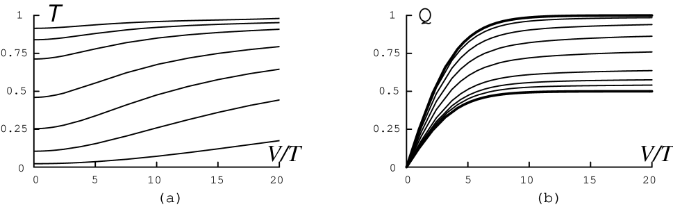
FIG. 2.: (a) Transparency of QPC2, $\tilde{\cal T}_{2}(v_{2}/T^{1/2},V/T)$ as a function of $V/T$ for different temperatures, $T/v_{2}^{2}=0.2,0.5,1,2,5,10,20$. The lowest temperatures have the lowest transparency. (b) Effective charge transmitted through QPC2, $\tilde{\cal Q}_{2}(v_{2}/T^{1/2},V/T)$ as a function of $V/T$ for the same set of temperatures as in (a). The lowest temperatures have the largest effective charge. The thick lines are the asymptotic limits ${\cal Q}(0,V/T)$ and ${\cal Q}(\infty,V/T)$ discussed in the text.

A striking feature of these curves is their behavior for large $V/T$. For each of the curves in Fig. 2a the transparency increases with increasing $V/T$ and eventually approaches 1. This is because the transmission through QPC2 becomes perfect for $V\gg v_{2}^{2}$. By contrast, the curves for the effective charge in Fig. 2b saturate at a constant value for $V/T\rightarrow\infty$. Thus, even though the transmission through QPC2 $\tilde{\cal T}_{2}(v_{2}/T^{1/2},\infty)=1$ is perfect, the charge $\tilde{\cal Q}_{2}(v_{2}/T^{1/2},\infty)$ of the transmitted particles is not equal to the charge $1/2$ of the quasiparticles incident on QPC2, but rather varies between $1/2$ and $1$ as the temperature is lowered. In striking contrast, at zero temperature equations (4.23) and (4.31) show that the effective charge of the transmitted particles $\tilde{\cal Q}_{2}^{\prime}(v_{2}/V^{1/2},\infty)=1$, independent of the voltage $V$. The scaling functions $\tilde{\cal Q}_{2}(v_{2}/T^{1/2},V/T)$ and $\tilde{\cal Q}_{2}^{\prime}(v_{2}/V^{1/2},V/T)$ thus show qualitatively different behavior. This is quite unusual, since usually the dependence of scaling functions on voltage and temperature are qualitatively similar. The origin of this behavior can be traced to the singular behavior of limit $T\rightarrow 0$ with fixed $V$:

$${\cal Q}(v_{2}=0,T\rightarrow 0,V) =1/2,$$ (73)

$${\cal Q}(v_{2}\rightarrow 0,T=0,V) =1.$$ (74)

The limits of $T\rightarrow 0$ and $v_{2}\rightarrow 0$ do not commute.

In section VB we will offer a physical interpretation of this peculiar behavior. However, before doing so it is important to ask whether it is an artifact of the chiral edge theory for $\nu=1/2$, or whether it also occurs more generally. In Fig. 3 we show perturbative calculations of $\tilde{\cal Q}_{3}(0,V/T)$ (Eq. 3.3) and $\tilde{\cal Q}_{3}(\infty,V/T)$ (Eqs. 3.21, 3.16, B.4). It seems quite plausible that for intermediate temperatures $\tilde{\cal Q}_{3}(v_{2}/T^{2/3},V/T)$ should interpolate smoothly between the two limits as in Fig. 2b. This does not exclude the possibility, however, that the curves cross over to $1/3$ for $V/T\gg v_{2}^{3/2}/T$. This is ruled out, however, by perturbation theory in $v_{2}$. Eq. 3.24 shows that for $v_{2}^{3/2}\ll T\ll V$, $\tilde{\cal Q}-1/3\propto v_{2}^{2}/T^{4/3}$. Thus, $\tilde{\cal Q}_{3}(v_{2}/T^{2/3},\infty)>1/3$ for finite $v_{2}$, and it presumably then crosses over to $1$ for $v_{2}\gg T^{2/3}$.

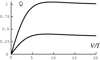
FIG. 3.: Scaling functions for the effective charge transmitted into lead 3 for $\nu=1/3$, $\tilde{\cal Q}_{3}(v_{2}/T^{2/3},V/T)$. The bottom curve is in the weak backscattering or high temperature limit, $\tilde{\cal Q}_{3}(0,V/T)$, whereas the top curve is in the low temperature limit, $\tilde{\cal Q}_{3}(\infty,V/T)$. Notice that in this limit of an opaque barrier ($v_{2}\gg T^{2/3}$) only electrons are transmitted through QPC2 when $V>>T$.

The small $v_{2}$ perturbation theory also gives a diverging correction to the transparency at zero temperature (Eq. 3.22). This divergence was absent for $\nu=1/2$. One may therefore worry that the transparency also goes to zero at $T=0$ for fixed $V$. However, this is contradicted by the small $t_{2}$ perturbation theory (3.14,3.18), which gives a finite transparency ${\cal T}_{3}\propto t_{2}^{2}V^{11/3}$ at $T=0$. It is most likely that the divergence for small $v_{2}$ signifies that transparency is not analytic at $v_{2}=0$. Such a non analyticity also occurs for $m=2$, where (4.23) gives ${\cal T}_{2}\sim 1-(v_{2}^{2}/V)\log V/v_{2}^{2}$.

The above arguments give strong evidence that the singular behavior at $T=0$ that we have established for $\nu=1/2$ also occurs for $\nu=1/3$ and other Laughlin filling fractions. Nonetheless, it would be desirable to obtain a full solution for $\nu=1/m$. Using the thermodynamic Bethe ansatz, Fendley, Ludwig and Saleur[13, 15] have calculated the current and noise for a single point contact, accounting for the full crossover between the weak backscattering and strong backcattering limits. It should be possible to generalize their formalism to the present 3-terminal geometry.

B Physical Picture for the $T\rightarrow 0$ limit

In this section we attempt to make sense out of the peculiar behavior we have established at zero temperature. We wish to understand how electrons can be transmitted through QPC2 into lead 3 even when the transparency of QPC2 is nearly perfect. We assume here that this effect occurs for $\nu=1/m$.

At zero temperature quasiparticles backscattered by QPC1 come in wave packets of charge $e/m$ and duration $\sim 1/V$ at a rate $\sim v_{1}^{2}V^{(2/m)-1}$. For $v_{1}\ll V^{1-(1/m)}$ the quasiparticle wave packets are independent and can be considered one at a time. The interaction of a quasiparticle with QPC2 presents a scattering problem. When a quasiparticle scatters from QPC2 it is natural to ask what comes out. Unlike the non interacting electron version of this problem the number of quasiparticles is not necessarily conserved in this scattering process. However, the total charge is conserved. We consider three processes. (1) The quasiparticle is transmitted with probability T into lead 3. (2) The quasiparticle is reflected with probability R into lead 1. (3) The quasiparticle is Andreev reflected with probability A. In this process an electron, with charge $e$ is transmitted into lead 3 while a hole with charge $(-1+1/m)e$ is reflected into lead 1. It is straightforward to show that if these are the only allowed processes (i.e. ${\sf T}+{\sf R}+{\sf A}=1$) the transparency is given by,

$${\cal T}={\sf T}+m{\sf A}.$$ (75)

Moreover, the effective charge will be,

$${\cal Q}={{\sf T}+m^{2}{\sf A}\over{m{\sf T}+m^{2}{\sf A}}}.$$ (76)

For $v_{2}\ll T^{1-1/m}$ we clearly have ${\sf R}={\sf A}=0$ and ${\sf T}=1$. On the other hand, at zero temperature our noise calculation shows that ${\sf T}=0$, since only electrons were found to be transmitted into lead 3. The transmitted current is thus apparently dominated by Andreev processes. This is no surprise in the large barrier limit $v_{2}\gg V^{1-1/m}$, where ${\cal T}$ is small, so that ${\sf A}$ is small and ${\sf R}\sim 1$. In the small barrier limit $v_{2}\ll V^{1-1/m}$, however, we have ${\cal T}\sim 1$. This then implies that ${\sf A}=1/m$ and ${\sf R}=1-1/m$. Thus, quite remarkably, the incident quasiparticle is either reflected or Andreev reflected with probabilities that have saturated at values which conspire to give perfect transmission of the current. Moreover, in this limit the time averaged current backscattered off QPC2 vanishes, although it will be noisy as we now detail.

A key feature of the Andreev processes is that the transmitted and reflected currents are correlated. These correlations give an unambiguous signature in the noise. We therefore propose that the noise be measured in both leads 1 and 3. It may be desirable to add an additional lead between leads 1 and 3 which can isolate the current reflected at QPC2. In any case, this will not affect the following zero temperature predictions. As above, the noise measured in lead 3 should reflect the charge $e$ of the Andreev transmitted electrons,

$$\Delta S_{33}=I_{3}.$$ (77)

The noise measured in lead 1, however, will be a combination of the charge $1/m$ reflected quasiparticles and the charge $(1/m)-1$ Andreev reflected holes. In terms of the measured currents, it will be given by

$$\Delta S_{11}=(1/m)\Delta I_{1}+(1-1/m)I_{3}.$$ (78)

Here $\Delta I_{1}$ is the current flowing into lead 1 due to the reflections from QPC2, that is $\Delta I_{1}=I_{1}+Ve^{2}/(mh)$. If an additional lead, say lead 4, is present between leads 1 and 3, then for $\Delta S_{44}$ one would have simply $\Delta I_{1}$ replaced by $I_{4}$ in equation (5.5). The cross correlations are determined solely by the Andreev processes,

$$\Delta S_{13}=-(1-1/m)I_{3}.$$ (79)

In the limit of weak pinch off for QPC2, we have $\Delta I_{1}=0$, at zero temperature. Nevertheless, the current flowing into lead 1 is noisy, with $\Delta S_{11}=-\Delta S_{13}=(1-1/m)\Delta S_{33}$. Thus, in this way one can prepare a noisy but zero time-averaged non-equilibrium current, present in the zero temperature limit where equilibrium current fluctuations vanish. While undoubtedly challenging, it would be fascinating to detect this effect and the presence of Andreev processes more generally.

C Relation to Existing Experiments

We close by commenting briefly on the implications of our results for the experiments of Comforti et al.[7]. It is clear that our results give no support to the notion of fractional charges traversing a nearly opaque barrier. So the interpretation of the data remains a puzzle. However, it is worthwhile to point out some possible sources of discrepancy.

The exact scaling functions for $m=2$ which we have computed are strictly speaking only applicable for a point contact which backscatters high energy (but still below the bulk FQHE gap) incident particles only weakly. A point contact which is strongly pinched off will not generally follow the universal crossover between weak and strong backscattering embodied in the scaling functions. Nevertheless, since our results show an absence of any subtle non-perturbative effects in the limit of weak tunneling through the point contact, it is difficult to imagine that this could modify our basic conclusion that only electrons can traverse an opaque barrier. It seems plausible that the experimentally observed charge of $0.45$ is a finite temperature crossover effect, which might well revert to a charge of $e$ as the temperature is lowered further. But it remains difficult reconciling a transmitted charge well below the electron charge for a point contact with such a small measured transparency of only $0.1$.

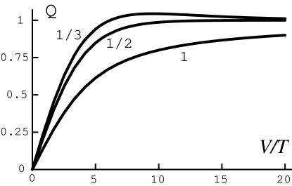
FIG. 4.: Scaling functions $\tilde{\cal Q}_{m}(v_{2}/T^{1-1/m},V/T)$ for the effective charge transmitted into lead 3 through QPC2 in the large barrier limit, $v_{2}/T^{1-1/m}\rightarrow\infty$. The three curves correspond to filling $\nu=1/m=1,1/2,1/3$ as labelled.

Comforti et al. [7] extracted the effective charge by fitting the measured $I(V,T)$ and $\Delta S(V,T)$ to an “independent particle model”, which is essentially the non interacting electron version ($m=1$) of the scaling functions $\tilde{I}_{m}(V/T)$ and $\tilde{S}_{m}$[19]. In Fig. 4 we compare the scaling functions for the effective charge in the large barrier limit $\tilde{\cal Q}_{m}(\infty,T/V)$ for $m=1$, $2$ and $3$. Here $\tilde{\cal Q}_{1}(\infty,x)=\coth x/2-2/x$, $\tilde{\cal Q}_{2}(\infty,x)=\tanh x/4$, and $\tilde{\cal Q}_{3}(\infty,x)$ is computed numerically as in Fig. 3. The curves clearly differ quantitatively. The results of this paper thus suggest an alternative method for analyzing the data: For fixed temperature plot the measured values of $\Delta S(V,T)/I(V,T)$ as a function of $V/T$ and compare with the scaling functions $\tilde{\cal Q}_{3}(0,V/T)$ and $\tilde{\cal Q}_{3}(\infty,V/T)$ in Fig. 3. For data taken at voltages $V\gtrsim 10T$ conclusions about the asymptotic charge for $V\gg T$ should not depend on the fitting method. But for smaller voltages there may well be a difference.

A Expectation values and Keldysh sums

In this appendix we demonstrate our technique for evaluating the expectation values and sums over Keldysh paths. In section A1 we do in detail the calculation for the small $t_{2}$ limit. This will establish our method, which can then be applied to the other calculations. In A2 we discuss the limit of small $v_{2}$. Finally in A3 we briefly discuss the calculations for the exact current and noise for $m=2$.

1 Small $t_{2}$ Perturbation Theory

In this section we provide some details of the calculation which leads from equation (3.8,3.9) to (3.10,3.11). Our starting point is the expansion of the current and noise to order $v_{1}^{2}t_{2}^{2}$. It is useful to introduce an index $\sigma=\pm$ which specifies the forward and backward paths of the Keldysh contour. Then, $\int_{C}d\tau\rightarrow\sum_{\sigma}\sigma\int dt$. For the variable $t_{1}$ (and $t_{2}$ for the noise) we introduce a dummy sum over $\sigma_{1}$ (and $\sigma_{2}$). In addition, we write the two terms in the tunneling Hamiltonian (3.4) and the current operator (3.6) as a sum over $s=\pm$. The current and noise can then be written,

$$I={1\over 4}v_{1}^{2}t_{2}^{2}\sum_{\{\sigma_{k},s_{k}\}}s_{1}\sigma_{2}\sigma_{3}\sigma_{4}\int d^{3}te^{-iV(s_{3}t_{3}+s_{4}t_{4})/m}\left\langle T_{C}\left[O^{s_{1}}_{2t}(\sigma_{1}t_{1})O^{s_{2}}_{2t}(\sigma_{2}t_{2})O^{s_{3}}_{1v}(\sigma_{3}t_{3})O^{s_{4}}_{1v}(\sigma_{4}t_{4})\right]\right\rangle_{0}$$ (A1)

$$\Delta S={1\over 8}v_{1}^{2}t_{2}^{2}\sum_{\{\sigma_{k},s_{k}\}}s_{1}s_{2}\sigma_{3}\sigma_{4}\int d^{3}te^{-iV(s_{3}t_{3}+s_{4}t_{4})/m}\left\langle T_{C}\left[O^{s_{1}}_{2t}(\sigma_{1}t_{1})O^{s_{2}}_{2t}(\sigma_{2}t_{2})O^{s_{3}}_{1v}(\sigma_{3}t_{3})O^{s_{4}}_{1v}(\sigma_{4}t_{4})\right]\right\rangle_{0}$$ (A2)

The three time integrals are over $t_{2}$, $t_{3}$ and $t_{4}$. Note, however, that due to invariance with respect to time translations they can be shifted to any three of the times $t_{1},t_{2},t_{3},t_{4}$. Clearly we must have $s_{1}+s_{2}=s_{3}+s_{4}=0$ in each of the sums on $\{s_{k}\}$. By appropriately re-labeling the integration variables, we may specify $s_{1}=-s_{2}=-s_{3}=s_{4}=+$.

$$I={1\over 2}v_{1}^{2}t_{2}^{2}\sum_{\{\sigma_{k}\}}(\sigma_{2}-\sigma_{1})\sigma_{3}\sigma_{4}\int d^{3}t\Pi(\{\sigma_{k},t_{k}\})e^{iVt_{34}/m}$$ (A3)

$$\Delta S={1\over 2}v_{1}^{2}t_{2}^{2}\sum_{\{\sigma_{k}\}}\sigma_{3}\sigma_{4}\int d^{3}t\Pi(\{\sigma_{k},t_{k}\})e^{iVt_{34}/m}$$ (A4)

where

$$\Pi(\{\sigma_{k},t_{k}\})=\left\langle T_{C}\left[O^{+}_{2t}(\sigma_{1}t_{1})O^{-}_{2t}(\sigma_{2}t_{2})O^{-}_{1v}(\sigma_{3}t_{3})O^{+}_{1v}(\sigma_{4}t_{4})\right]\right\rangle_{0}.$$ (A5)

$\Pi(\{\sigma_{k},t_{k}\})$ is computed by first computing the imaginary time ordered correlation function.

$$\Pi(\{\tau_{k}\})=\left\langle T_{\tau}\left[O^{+}_{2t}(\tau_{1})O^{-}_{2t}(\tau_{2})O^{-}_{1v}(\tau_{3})O^{+}_{1v}(\tau_{4})\right]\right\rangle_{0}.$$ (A6)

The expectation value factorizes into three terms,

$$\Pi(\{\tau_{k}\})={\left\langle T_{\tau}\left[e^{i(\phi_{1}(0,\tau_{3})-\phi_{1}(0,\tau_{4}))}\right]\right\rangle_{0}\left\langle T_{\tau}\left[e^{i(\phi_{3}(L,\tau_{1})-\phi_{3}(L,\tau_{2}))}\right]\right\rangle_{0}\left\langle T_{\tau}\left[e^{i(\phi_{2}(L,\tau_{1})-\phi_{2}(L,\tau_{2})-\phi_{2}(0,\tau_{3})+\phi_{2}(0,\tau_{4}))}\right]\right\rangle_{0}\over{(2\pi\eta)^{2m+2/m}}}$$ (A7)

where $T_{\tau}$ signifies time ordering in imaginary time. Using the Hamiltonian (2.1) it is straightforward to show that

$$\Pi(\{\tau_{k}\})={(T/2)^{2m+2/m}\over{\sin^{2m}\pi T(\eta+\sigma_{12}\tau_{12})\sin^{2/m}\pi T(\eta+\sigma_{34}\tau_{34})}}{\sin\pi T(\eta+\sigma_{13}(\tau_{13}-iL))\sin\pi T(\eta+\sigma_{24}(\tau_{24}-iL))\over{\sin\pi T(\eta+\sigma_{23}(\tau_{23}-iL))\sin\pi T(\eta+\sigma_{14}(\tau_{14}-iL))}}.$$ (A8)

Here $\sigma_{ij}={\rm sign}(\tau_{i}-\tau_{j})$ reflects ordering of the operators in the imaginary time ordered product.

The real time correlation functions are determined by taking $\tau_{ij}\rightarrow it_{ij}$. The operator ordering is now determined by the time ordering on the Keldysh contour. Thus $\sigma_{ij}=\pm 1$ depending on whether the time $t_{i}\sigma_{i}$ comes later or earlier than $t_{j}\sigma_{j}$ on the Keldysh contour. $\sigma_{ij}$ now depends on the Keldysh paths $\sigma_{i}$, $\sigma_{j}$ as well as the sign of the time difference $s_{ij}={\rm sign}(t_{i}-t_{j})$. Explicitly it may be written

$$\sigma_{ij}={1\over 2}\left[(\sigma_{j}-\sigma_{i})+s_{ij}(\sigma_{i}+\sigma_{j})\right].$$ (A9)

In the limit of large $L$ the only times to contribute will be those with $t_{1,2}\sim t_{3,4}+L$. Therefore from (A10), $\sigma_{13}=\sigma_{23}=\sigma_{3}$ and $\sigma_{14}=\sigma_{24}=\sigma_{4}$. The real time correlation function may then be expressed in the form

$$\Pi(\{\sigma_{k},t_{k}\})=G^{\sigma_{12}}_{2m}(t_{12})G^{\sigma_{34}}_{2/m}(t_{34})K_{1}^{\sigma_{3}\sigma_{4}}$$ (A10)

with

$$G_{\alpha}^{\pm}(t)=\left({T\over{2\sin\pi T(\eta\pm it)}}\right)^{\alpha}$$ (A11)

and

$$K^{\sigma_{3}\sigma_{4}}_{\alpha}=\left({\sin\pi T(\eta+i\sigma_{3}(t_{13}-L))\sin\pi T(\eta+i\sigma_{4}(t_{24}-L))\over{\sin\pi T(\eta+i\sigma_{3}(t_{23}-L))\sin\pi T(\eta+i\sigma_{4}(t_{14}-L))}}\right)^{\alpha}.$$ (A12)

$G_{\alpha}^{\pm}(t)$ may be interpreted as a two point Green’s function more commonly referred to as $G^{<,>}(t)$. For instance $G_{2m}^{+}(t)=\left\langle O_{2t}^{+}(t)O_{2t}^{-}(0)\right\rangle_{0}$ and $G_{2m}^{-}(t)=\left\langle O_{2t}^{-}(0)O_{2t}^{+}(t)\right\rangle_{0}$.

Substituting (A10-A12) into (A3) the sums on $\{\sigma_{k}\}$ may be evaluated giving

$$I=v_{1}^{2}t_{2}^{2}\int d^{3}te^{iVt_{34}/m}(G^{+}_{2m}(t_{12})-G^{-}_{2m}(t_{12}))\biggl{[} G^{+}_{2/m}(t_{34})\left(K_{1}^{-+}+{1\over 2}(K_{1}^{++}+K_{1}^{--})+{1\over 2}s_{34}(K_{1}^{++}-K_{1}^{--})\right)$$ (A13)

$$+ G^{-}_{2/m}(t_{34})\left(K_{1}^{+-}+{1\over 2}(K_{1}^{++}+K_{1}^{--})-{1\over 2}s_{34}(K_{1}^{++}-K_{1}^{--})\right)\biggr{]}.$$ (A14)

This equation may be simplified by considering the dependence of the integrand on the “average time difference” $t_{0}=(t_{1}+t_{2}-t_{3}-t_{4})/2$. $t_{0}$ enters the only in the form $L\rightarrow L-t_{0}$ and may be interpreted as the time it takes quasiparticles to propagate between the two junctions. It can be shown by contour integration that

$$\int dt_{0}(K^{++}-K^{--})=0.$$ (A15)

This allows us to rewrite (A13) in the simpler form,

$$I=v_{1}^{2}t_{2}^{2}\int dt_{2}dt_{3}dt_{4}e^{iVt_{34}/m}\left(G_{2m}^{+}(t_{12})-G_{2m}^{-}(t_{12})\right)\left[G_{2/m}^{+}(t_{34})(K_{1}^{-+}-K_{1}^{--})+G_{2/m}^{-}(t_{34})(K_{1}^{+-}-K_{1}^{++})\right].$$ (A16)

The sum over $\sigma_{k}$ for the noise is almost the same, except for the first term in (A3). This gives

$$\Delta S=v_{1}^{2}t_{2}^{2}\int dt_{2}dt_{3}dt_{4}e^{iVt_{34}/m}\left(G_{2m}^{+}(t_{12})+G_{2m}^{-}(t_{12})\right)\left[G_{2/m}^{+}(t_{34})(K_{1}^{-+}-K_{1}^{--})+G_{2/m}^{-}(t_{34})(K_{1}^{+-}-K_{1}^{++})\right].$$ (A17)

Finally, in equations (3.10,3.11) we have shifted $t_{1,2}\rightarrow t_{1,2}-L$ to eliminate the variable $L$.

2 Current and Noise for $v_{2}=0$

Here we briefly outline the calculation of the current and noise when the second junction transmits perfectly. Similar results have been obtained in earlier for the single junction[4, 8, 9]. We include the calculation here because the result is slightly different and because we use a somewhat different method, which will be useful when generalizing to finite $v_{2}$.

We express the current $I=I_{3}$ in terms of incident currents and the current backscattered at the first junction,

$$\hat{I}=\hat{I}_{2\rm in}-\hat{I}_{3\rm in}+\hat{I}_{b1}$$ (A18)

where $I_{2,3\rm in}=\partial_{x}\phi_{2,3}/2\pi$ are the currents carried by the chiral edge states incident from leads 2 and 3. The current backsattered at the first junction is

$$\hat{I}_{b1}=-i(v_{1}/m)(O_{1v}^{+}e^{-iVt/m}-O_{1v}^{-}e^{iVt/m}).$$ (A19)

The backscattered current is related to the voltage drop across the junction, discussed in Ref. [4]. For the current the first two terms in (A18) cancel, and we have $I=\langle I_{b1}\rangle$. This may be evaluated using the procedure in appendix A1 to be

$$I={v_{1}^{2}\over m}\int dte^{iVt/m}\left(G^{+}_{2/m}(t)-G^{-}_{2/m}(t)\right)$$ (A20)

with $G^{\pm}_{2/m}(t)$ given in (A11). Evaluation of the integral gives the result quoted in (3.1).

The excess noise contains two contributions,

$$\Delta S=\Delta S_{b1,b1}+2\Delta S_{b1,2\rm in}.$$ (A21)

The fluctuation in the backscattered current $\Delta S_{b1,b1}=(1/2)\int dt\langle\hat{I}_{b1}(t)\hat{I}_{b1}(0)\rangle$ is related to the voltage fluctuations across the junction. It has the form (check sign),

$$\Delta S_{b1,b1}={v_{1}^{2}\over m^{2}}\int dte^{iVt/m}\left(G^{+}_{2/m}(t)+G^{-}_{2/m}(t)\right).$$ (A22)

Using the fact that $G^{-}(t+i/T)=G^{+}(t)$ it is straightforward to establish that $\delta S_{bb}=(I/m)\coth V/2mT$. Physically, the two terms in (A19) and (A21) describe the rates for forward and backward tunneling of quasiparticles across the voltage difference $V$ which are related by a factor $e^{V/mT}$.

The second term, $\Delta S_{b1,2\rm in}=(1/2)\int dt\langle\{\hat{I}_{b1}(t),\hat{I}_{2\rm in}(0)\}\rangle$ gives the cross correlation between the backscattered current and thermal fluctuations in the current incident from lead 2. This cross correlation can be shown to have the form

$$\Delta S_{b1,2\rm in}=T{\partial\langle I_{b1}\rangle\over{\partial V_{2}}}$$ (A23)

In equilibrium, $V\rightarrow 0$ this is simply a statement of the fluctuation dissipation theorem. However, as shown in Ref. [4], it is also valid for $V>0$.

Combining (A21) and (A22) we get the result quoted in (3.2). Note that the other terms present in $S$ do not contribute to the excess noise. In particular the current incident from lead 3 will have no correlation with $I_{b}$.

3 Small $v_{2}$ perturbation theory

When $v_{2}$ is finite we write the current as

$$\hat{I}=I_{2,\rm in}-I_{3,\rm in}+I_{b1}-I_{b2},$$ (A24)

where the current backscattered at the second junction is

$$\hat{I}_{b2}=-i(v_{2}/m)(O_{2v}^{+}-O_{2v}^{-}).$$ (A25)

The average current at order $v_{2}^{2}$ is then given by $I=I_{b2}$. This may be computed along the lines of the previous section. The structure is almost identical to (A15), except the dimensions of the operators is changed. We find

$$I_{b2}={v_{1}^{2}v_{2}^{2}\over m}\int d^{3}te^{i(V_{12}t_{34}-V_{32}t_{12})/m}\left(G_{2/m}^{+}(t_{12})-G_{2/m}^{-}(t_{12})\right)\left[G_{2/m}^{+}(t_{34})(K_{1/m}^{-+}-K_{1/m}^{--})+G_{2/m}^{-}(t_{34})(K_{1/m}^{+-}-K_{1/m}^{++})\right].$$ (A26)

For use in the next section we have included voltages $V_{k}$ in all three contacts, and $V_{kl}=V_{k}-V_{l}$. The current is evaluated with $V_{2}=V_{3}=0$ and $V_{1}=V$.

From (A23), the nonzero contributions to the excess noise at order $v_{2}^{2}$ will be given by

$$\Delta S=\Delta S_{b2,b2}-2\Delta S_{b1,b2}-2\Delta S_{b2,2\rm in}+2\Delta S_{b2,3\rm in}$$ (A27)

As in the previous section, the cross correlations with the incident currents have the form

$$\Delta S_{b2,k\rm in}=T{\partial I_{b2}\over{\partial V_{k}}}$$ (A28)

for $k=1,2$. In addition we find

$$\Delta S_{b2,b2}={v_{1}^{2}v_{2}^{2}\over m^{2}}\int d^{3}te^{iVt_{34}/m}\left(G_{2/m}^{+}(t_{12})+G_{2/m}^{-}(t_{12})\right)\left[G_{2/m}^{+}(t_{34})(K_{1/m}^{-+}-K_{1/m}^{--})+G_{2/m}^{-}(t_{34})(K_{1/m}^{+-}-K_{1/m}^{++})\right].$$ (A29)

The cross correlation is given by

$$\Delta S_{b2,b1}={v_{1}^{2}v_{2}^{2}\over m^{2}}\int d^{3}te^{iVt_{34}/m}\left(G_{2/m}^{+}(t_{12})-G_{2/m}^{-}(t_{12})\right)\left[G_{2/m}^{+}(t_{34})K_{1/m}^{-+}-G_{2/m}^{-}(t_{34})K_{1/m}^{+-}\right].$$ (A30)

4 Current for $m=2$

In this section provide details of the calculation relating (4.17) to (4.18) in the evaluation of

$$A(x_{1},x_{2})=\langle O_{2v}^{+}(x_{1})O_{2v}^{-}(x_{2})-O_{2v}^{-}(x_{1})O_{2v}^{+}(x_{2})\rangle.$$ (A31)

The procedure is quite similar to that of appendix A1. We begin by rewriting (4.17) as

$$A(x_{1},x_{2})={1\over 2}v_{1}^{2}\sum_{\{\sigma_{k}\}}(\sigma_{2}-\sigma_{1})\sigma_{3}\sigma_{4}\int dt_{3}dt_{4}e^{iVt_{34}/m}\Pi(\{\sigma_{k},t_{k},x_{k}\})$$ (A32)

with

$$\Pi(\{\sigma_{k},t_{k},x_{k}\})=\left\langle T_{C}\left[O^{+}_{2v}(\sigma_{1}0,x_{1})O^{-}_{2v}(\sigma_{2}0,x_{2})O^{-}_{1v}(\sigma_{3}t_{3})O^{+}_{1v}(\sigma_{4}t_{4})\right]\right\rangle_{0}.$$ (A33)

The correlation function has the same structure as (A5)

$$\Pi(\{\sigma_{k},t_{k},x_{k}\})=G^{\sigma_{12}}_{1}(x_{12})G^{\sigma_{34}}_{1}(t_{34})K_{1/2}^{\sigma_{3}\sigma_{4}}$$ (A34)

with $G^{\pm}(x)$ and $K_{1/2}^{\sigma_{3}\sigma_{4}}$ given in (A12,13) with $t_{1,2}$ replaced by $x_{1,2}$. Summing on the Keldysh indices we find,

$$A(x_{1},x_{2})=v_{1}^{2}\int dt_{3}dt_{4}e^{iVt_{34}/m}\left(G_{1}^{+}(x_{12})-G_{1}^{-}(x_{12})\right)\left[G_{1}^{+}(x_{34})(K_{1/2}^{-+}-K_{1/2}^{--})+G_{1}^{-}(t_{34})(K_{1/2}^{+-}-K_{1/2}^{++})\right].$$ (A35)

The first term in the integrand can be interpreted as the zeroth order expectation value,

$$A^{0}(x_{1},x_{2})=\left\langle O_{2v}^{+}(x_{1})O_{2v}^{-}(x_{2})-O_{2v}^{-}(x_{1})O_{2v}^{+}(x_{2})\right\rangle_{0}=G_{1}^{+}(x_{12})-G_{1}^{-}(x_{12}).$$ (A36)

5 Noise for $m=2$

Calculation of the expectation values $A_{1,2}(\{x_{k}\})$ in equations (4.25) and (4.26) of section IVB can be done in the same manner as the previous section. Again, the expectation value can be factored into a zeroth order expectation value times an integral. We find

$$A_{1,2}(\{x_{k}\})=v_{1}^{2}A_{1,2}^{0}(\{x_{k}\})\int dt_{5}dt_{6}e^{iVt_{34}/2}\left[G^{+}(t_{56})(K^{-+}-K^{--})+G^{-}(t_{56})(K^{+-}-K^{++})\right]$$ (A37)

where $G^{\pm}(t)$ is the same as (A12) and

$$K^{\sigma_{5}\sigma_{6}}=\left({\sin\pi T(\eta+i\sigma_{5}z_{15})\sin\pi T(\eta+i\sigma_{5}z_{35})\sin\pi T(\eta+i\sigma_{6}z_{26})\sin\pi T(\eta+i\sigma_{6}z_{46})\over{\sin\pi T(\eta+i\sigma_{5}z_{25})\sin\pi T(\eta+i\sigma_{5}z_{45})\sin\pi T(\eta+i\sigma_{6}z_{16})\sin\pi T(\eta+i\sigma_{6}z_{36})}}\right)^{1/2},$$ (A38)

where we use the notation $z_{ij}=x_{i}-t_{j}$. The zeroth order expectation values can be evaluated using Wick’s theorem for the fermionic operators $O_{2v}^{\pm}$,

$$A_{1}^{0}(\{x_{k}\})=\left(G^{+}(x_{12})-G^{-}(x_{12})\right)\left(G^{+}(x_{34})-G^{-}(x_{34})\right)+4G^{+}(x_{14})G^{+}(x_{23})$$ (A39)

$$A_{2}^{0}(\{x_{k}\})=G^{+}(x_{14})G^{-}(x_{23})-G^{+}(x_{12})G^{+}(x_{34})+G^{-}(x_{14})G^{+}(x_{23})-G^{-}(x_{12})G^{-}(x_{34}).$$ (A40)

B Evaluation of Integrals

1 Small $t_{2}$ Perturbation Theory

In this section we simplify the integrals (3.10) and (3.11). One of the integrals can be easily done because

$$K_{1}^{-+}-K_{1}^{--}=(K_{1}^{+-}-K_{1}^{++})^{*}=-(2/T)\delta(t_{14}){\sin\pi Tit_{34}\ \ \sin\pi Tit_{12}\over{\sin\pi T(\eta-it_{23})}}$$ (B1)

This allows us to write the current ($I=C_{-}$) and noise ($S=C_{+}$) as

$$C_{\pm}=-v_{1}^{2}t_{2}^{2}\int dt_{2}dt_{3}e^{iVt_{3}/m}\left(G^{+}_{2m-1}(t_{2})\pm G^{-}_{2m-1}(t_{2})\right)\left(G^{+}_{2/m-1}(t_{3})G^{-}_{1}(t_{23})+G^{-}_{2/m-1}(t_{3})G^{+}_{1}(t_{23})\right).$$ (B2)

Defining $u=\pi Tt_{2}\pm i\pi/2$ for the terms involving $G^{\pm}_{2m-1}(t_{2})$ and $v=\pi Tt_{3}\pm i\pi/2$ for the terms involving $G^{\pm}_{2/m-1}(t_{3})$, the terms in the integral can be combined and written in the scaling form $C_{\pm}(V,T)=v_{1}^{2}t_{2}^{2}T^{2m+2/m-3}\tilde{C}_{\pm}(V/T)$ with

$$\tilde{C}_{t,m}(X)={2^{2-2m-2/m}\sinh(X/2m)\over\pi^{2}}\int_{-\infty}^{\infty}dudv{e^{iXv/m\pi}\over{\cosh^{2m-1}u\cosh^{2/m-1}v}}\left({1\over{\sin(\eta+i(u-v))}}\mp{1\over{\sin(\eta-i(u-v))}}\right)$$ (B3)

The integrals for $\tilde{I}_{t,m}(V/T)$ can be evaluated because the factor in parentheses is a $\delta$ function. The result is given in (3.16). The integral for $\tilde{S}_{t,m}(V/T)$ has the form

$$\tilde{S}_{t,m}(X)={2^{3-2m-2/m}\sinh(X/2m)\over{\pi^{2}}}\int_{-\infty}^{\infty}dudv{\sin Xv/m\pi\over{\cosh^{2m-1}u\cosh^{2/m-1}v\sinh(u-v)}}.$$ (B4)

This is evaluated numerically in section V.

In special cases the above results simplify. For $m=1$ we find $\tilde{I}_{t,1}(X)=X/2\pi$ and $\tilde{S}_{t,1}(X)=(X\coth X/2-2)/2\pi$. Thus,

$$\tilde{\cal Q}_{1}(X,\infty)=\coth(X/2)-2/X.$$ (B5)

These results are the same as those you get for non interacting electrons[19]. For $m=2$ we find $\tilde{I}_{t,2}(X)=(1/32\pi^{2})(X^{2}+4\pi^{2})\tanh(X/4)$ and $\tilde{S}_{t,2}(X)=(1/32\pi^{2})(X^{2}+4\pi^{2})\tanh^{2}(X/4)$. Thus,

$$\tilde{\cal Q}_{2}(X,\infty)=\tanh(X/4).$$ (B6)

2 Small $v_{2}$ Perturbation Theory

In this section we evaluate the integrals for the correction to the current and noise at order $v_{2}^{2}$. Since the purpose of this calculation is to establish the divergence of the perturbation theory for $T\rightarrow 0$ with fixed $V$, we will focus on the limit $V\gg T$.

We begin with Eq. A26 for the current. For $V/T\rightarrow\infty$ and $m>1$ the integral over $t_{34}$ is dominated by the region with $t_{34}\ll t_{31},t_{32}$, where $K^{\sigma_{3}\sigma_{4}}_{1/m}$ is independent of $t_{34}$. The integral over $t_{3}$ can then be evaluated (with $t_{4}=0$) giving,

$$I_{b2}=v_{1}^{2}v_{2}^{2}{(V/(2\pi m))^{2/m-1}\over{\Gamma(2/m)}}\int dt_{1}dt_{2}(G^{+}_{2/m}(t_{12})-G^{-}_{2/m}(t_{12}))(K^{-+}_{1/m}-K^{--}_{1/m})$$ (B7)

Using the fact that $G^{\pm}_{2/m}(t_{12})=e^{\mp is_{12}\pi/m}(T/2\sin\pi T|t_{12}|)^{2/m}$ and $K^{\sigma_{3}\sigma_{4}}_{1/m}=e^{i(\pi/2m)(\sigma_{3}-\sigma_{4})(s_{10}-s_{20})}$ (for $t_{3}=t_{4}=0$) we then obtain

$$I_{b2}=a_{m}v_{1}^{2}v_{2}^{2}V^{2/m-1}T^{2/m-2}$$ (B8)

with

$$a_{m}={1\over{(2\pi m)^{2/m}}}{\Gamma(1/m)^{2}\over{\Gamma(2/m)^{2}}}\sin(2\pi/m)$$ (B9)

Note that $a_{2}=0$. The $v_{2}^{2}$ correction to the current vanishes for $V\gg T$ for $m=2$.

A similar calculation for the noise gives

$$\Delta S=b_{m}v_{1}^{2}v_{2}^{2}V^{2/m-1}T^{2/m-2}.$$ (B10)

$b_{m}$ has contributions from the four terms in (A23), $b_{m}=b_{b2,b2,m}-2b_{b1,b2,m}+2b_{b2,2{\rm in},m}-2b_{b2,3{\rm in},m}$. The first two terms can be evaluated by applying the analysis in eq (B7) to equations (A28) and (A29). We find $b_{b2,b2,m}=b_{b1,b2,m}=a_{m}/m$, with $a_{m}$ given above. The third and fourth terms are evaluated by differentiating with respect to $V_{2}$ and $V_{3}$. The dominant contribution for $V\gg T$ is due the term where the differentiation pulls down a factor of $it_{12}/m$. Following the above analysis we then find

$$b_{m}={4\over{m(2\pi m)^{2/m}}}{\Gamma(1/m)^{2}\over{\Gamma(2/m)^{2}}}{\sin^{3}(\pi/m)\over{\cos(\pi/m)}}\left({2\over\pi^{2}}\psi^{\prime}(1/m)-1\right)-{a_{m}\over m}.$$ (B11)

where $\psi^{\prime}(x)$ is the derivative of the digamma function. The coefficients can be evaluated for $m=2,3$ to be $a_{2}=0$, $b_{2}=14\zeta(3)/\pi^{3}=0.5428$. $a_{3}=0.4786$, $b_{3}=0.8414$. The effective charge then has the expansion

$$\tilde{\cal Q}_{m}(v_{2}/T_{1-1/m},V/T\rightarrow\infty)={1\over m}+c_{m}{v_{2}^{2}\over T^{2-2/m}}$$ (B12)

with

$$c_{m}={2\over{m\pi}}{\sin^{3}(\pi/m)\over{\cos(\pi/m)}}{\Gamma(1/m)^{2}\over{\Gamma(2/m)}}\left({2\over\pi^{2}}\psi^{\prime}(1/m)-1\right).$$ (B13)

Then $c_{1}=0$, $c_{2}=28\zeta(3)/\pi^{3}=1.0855$ and $c_{3}=1.5279$.

3 Exact Current $m=2$

In this section we evaluate the integrals for the exact calculation of the current for $m=2$ described in section IVB. Combining (4.15) and (4.18) we find

$$I={v_{1}^{2}\over 2L}\int dx_{1}dx_{2}d_{1}(x_{12})\left(G_{1}^{+}(x_{12})-G_{1}^{-}(x_{12})\right)\int dt_{3}dt_{4}e^{iVt_{34}/2}\left[G_{1}^{+}(t_{34})\left(K_{1/2}^{-+}-K_{1/2}^{--}\right)+G_{1}^{-}(t_{34})\left(K_{1/2}^{+-}-K_{1/2}^{++}\right)\right].$$ (B14)

Using the fact that $G_{1}^{+}(t_{34}-i\pi T)=G_{1}^{-}(t_{34})$ and similar identities for $K$, we found it convenient to rewrite the integral over $t_{3,4}$ as

$$\tanh{V\over 4T}\int dt_{3}dt_{4}e^{iVt_{34}/2}\left[G_{1}^{+}(t_{34})\left(K_{1/2}^{-+}-K_{1/2}^{--}\right)-G_{1}^{-}(t_{34})\left(K_{1/2}^{+-}-K_{1/2}^{++}\right)\right].$$ (B15)

The integration is then simplified using $G_{1}^{+}(t_{34})+G_{1}^{-}(t_{34})=\pi T\delta(t_{34})$. The term involving $\delta(t_{34})$ does not contribute because $K_{1/2}^{-+}-K_{1/2}^{--}-K_{1/2}^{+-}+K_{1/2}^{++}=0$ for $t_{3}=t_{4}$. Then the integral over $t_{3,4}$ is then

$$2\tanh{V\over 4T}\int dt_{3}dt_{4}e^{-iVt_{34}/2}\left(G_{1}^{+}(t_{34})-G_{1}^{-}(t_{34})\right)\rho_{12}(t_{3},t_{4})$$ (B16)

with

$$\rho_{12}(t_{3},t_{4})={1\over 4}\left(K_{1/2}^{-+}+K_{1/2}^{+-}-K_{1/2}^{--}-K_{1/2}^{++}\right).$$ (B17)

This integral can be further simplified by symmetrizing the integrand with respect to permutations of $t_{3}$ and $t_{4}$ and permutations of $x_{1}$ and $x_{2}$, and then restricting the integration region to be $x_{1}>x_{2}$ and $t_{3}>t_{4}$ We then set $t_{4}=0$ to cancel the $L$. Using a trigonometric identity it can be shown that

$$\rho_{12}(t_{3},0)-\rho_{21}(t_{3},0)={\sinh\pi Tt_{3}\sinh\pi Tx_{12}\over{\sqrt{\sinh\pi T(x_{1}-t_{3})\sinh\pi T(t_{3}-x_{2})\sinh\pi T(x_{1})\sinh\pi T(-x_{2})}}}$$ (B18)

when $x_{2}<0<t_{3}<x_{1}$ and $0$ otherwise. We then find

$$I=2v_{1}^{2}T^{2}\tanh{V\over 4T}\int_{0}^{\infty}dx_{1}\int_{-\infty}^{0}dx_{2}\int_{0}^{x_{1}}dt_{3}{\left(\delta(x_{12})-v_{2}^{2}e^{-2v_{2}^{2}|x_{12}|}\right)\cos(Vt_{3}/2)\over\sqrt{\sinh\pi T(x_{1}-t_{3})\sinh\pi T(t_{3}-x_{2})\sinh\pi Tx_{1}\sinh\pi T(-x_{2})}}$$ (B19)

The two terms in parentheses in (B19) can be interpreted as the incident and backscattered currents for the second junction, $I=I_{\rm in}-I_{b2}$. The $\delta$ function term can be evaluated using a concrete regularization of the $\delta$ function, $\delta(x_{12})=\lim_{Z\rightarrow\infty}Z\exp(-2Z|x_{12}|).$ This gives

$$I_{\rm in}={v_{1}^{2}\over 2}\tanh{V\over 4T},$$ (B20)

in agreement with the current calculated for $v_{2}=0$ in section III for $m=2$.

For the second term we define new variables, $y_{1}=\pi T(x_{1}-t_{3})$, $y_{2}=-\pi Tx_{2}$, $u=\pi Tt_{3}$. The backscattered current can then be written in the form,

$$I_{b2}={2v_{1}^{2}v_{2}^{2}\over{\pi^{3}T}}\tanh{V\over 4T}\int_{0}^{\infty}dudy_{1}dy_{2}{e^{-2(u+y_{1}+y_{2})v_{2}^{2}/\pi T}\cos(Vu/2\pi T)\over{\sqrt{\sinh y_{1}\sinh(u+y_{1})\sinh y_{2}\sinh(u+y_{2})}}}$$ (B21)

.

Combining (B20) and (B21) the final result can be cast in the scaling form $I(V,T)=v_{1}^{2}\tilde{I}(v_{2}/T^{1/2},V/T)$ with

$$\tilde{I}_{2}(v_{2}/T^{1/2},V/T)={1\over 2}\tanh{V\over 4T}\left(1-{4v_{2}^{2}\over{\pi^{3}T}}\int_{0}^{\infty}du\cos{uV\over 2\pi T}\left[\int_{0}^{\infty}dy{e^{-(u+2y)v_{2}^{2}/\pi T}\over\sqrt{\sinh y\sinh(y+u)}}\right]^{2}\right).$$ (B22)

The integrals can be evaluated in the limit of large and small $v_{2}$, with results quoted in section IIIB. In the limit of zero temperature, the integrals simplify. Rescaling the integration variables by $v_{2}^{2}/\pi T$ we may write the current in the form (4.20) with

$$\tilde{I}_{2}^{\prime}(v_{2}/V^{1/2},\infty)={1\over 2}\left(1-{4\over{\pi^{2}}}\int_{0}^{\infty}du\cos{Vu\over{2v_{2}^{2}}}\left[\int_{0}^{\infty}dy{e^{-(u+2y)}\over\sqrt{y(y+u)}}\right]^{2}\right).$$ (B23)

The integral over $y$ in the square brackets is a Bessel function, $K_{0}(u)$. The remaining integral over $u$ then gives

$$\tilde{I}_{2}^{\prime}(v_{2}/V^{1/2},\infty)={1\over 2}\left[1-{2\over\pi}{\bf K}\left(-{V^{2}\over{16v_{2}^{4}}}\right)\right].$$ (B24)

where ${\bf K}$ is the elliptic integral of the second kind.

4 Exact Noise $m=2$

Combining (4.24) and (A37) and using the transformations (B9-B12) the noise may be written,

$$\Delta S={v_{1}^{2}\over 2L}\tanh{V\over 4T}\int d^{4}xdt_{5}dt_{6}F(\{x_{k}\})\left(G_{1}^{+}(t_{56})-G_{1}^{-}(t_{56})\right)\rho(\{x_{k}\},t_{5},t_{6})e^{iVt_{56}/2}$$ (B25)

where as $\rho(\{x_{k}\},t_{5},t_{6})=(K_{1/2}^{-+}+K_{1/2}^{+-}-K_{1/2}^{--}-K_{1/2}^{++})/4$ with $K$ given in (A38) and

$$F(\{x_{k}\})=d_{1}(x_{12})d_{1}(x_{34})A_{1}^{0}(\{x_{k}\})-d_{2}(x_{13})d_{2}(x_{24})A_{2}^{0}(\{x_{k}\}).$$ (B26)

$A_{1,2}^{0}(\{x_{k}\})$ is given in (A39,40), and $d_{1,2}(x)$ are in (4.13,4.14). It is again useful to symmetrize the integrand with respect to permutations of $x_{1},x_{2},x_{3},x_{4}$ and permutations of $t_{5}$ and $t_{6}$. $t_{6}$ is then set to zero, and we define $y_{k}=\pi Tx_{k}$, $u=\pi Tt_{5}$. After some lengthy algebra one finds,

$$\Delta S={2v_{1}^{2}\over\pi^{3}}\tanh{V\over 4T}\int_{R}d^{4}ydu\Theta(\{y_{k}\},u)\sin{Vu\over{2\pi T}}{D(\{y_{k}\})M(y_{1},y_{3},u)M(y_{2},y_{4},u)\over{\sinh u\sinh y_{13}\sinh\pi y_{24}}},$$ (B27)

where the integration region $R$ is $y_{1}>y_{2}>y_{3}>y_{4}$ and $u>0$. In addition

$$D(\{y_{k}\})=\delta_{12}\delta_{34}+{v_{2}^{2}\over{\pi T}}\left(\delta_{23}e^{-2y_{14}v_{2}^{2}/\pi T}-\delta_{12}e^{-2y_{34}v_{2}^{2}/\pi T}-\delta_{34}e^{-2y_{12}v_{2}^{2}/\pi T}\right)+{v_{2}^{4}\over{\pi^{2}T^{2}}}e^{-2(y_{12}+y_{34})v_{2}^{2}/\pi T},$$ (B28)

$$M(y_{i},y_{j},u)={\sinh y_{i}\sinh(y_{j}-u)+\sinh y_{j}\sinh(y_{i}-u)\over\sqrt{|\sinh y_{i}\sinh y_{j}\sinh(y_{j}-u)\sinh(y_{i}-u)|}},$$ (B29)

and

$$\Theta(\{y_{k}\},u)=\left\{\begin{array}[]{cl}1&{\rm for}\quad y_{1}>u>y_{2}>y_{3}>0>y_{4}\\ -1&{\rm for}\quad y_{1}>y_{2}>y_{3}>u>0>y_{4}\\ -1&{\rm for}\quad y_{1}>u>0>y_{2}>y_{3}>y_{4}\\ 0&{\rm otherwise}.\end{array}\right.$$ (B30)

We have evaluated these integrals numerically to obtain the scaling function $\tilde{S}(v_{2}/T^{1/2},V/T)$. The results were discussed in section V.

In the limit of zero temperature it is possible to obtain an analytic solution. Due to the complexity of the integral and to explain a subtlety in dealing with the $\delta$ functions we divide the result into three contributions by writing $I=I_{\rm in}-I_{b2}$, where $I_{\rm in}$ is the current incident on the 2nd junction and $I_{b2}$ is the current backscattered by the second junction. The noise is then a sum of three terms,

$$\Delta S=\Delta S_{\rm in,in}-2\Delta S_{\rm in,b2}+\Delta S_{\rm b2,b2}.$$ (B31)

These three terms arise from the three terms in $D(\{x_{k}\})$.

The term with two $\delta$ functions gives the noise incident on the second junction. It can be evaluated using the regularization $\delta_{ij}\equiv\delta(y_{ij})=\lim_{Z\rightarrow\infty}Z\exp(-2Z|y_{ij}|)$. We find

$$\Delta S_{\rm in,in}={v_{1}^{2}\over 4}\tanh^{2}({V\over 4T}),$$ (B32)

in agreement with the result for $v_{2}=0$ discussed in section IIIA. Thus at zero temperature $\Delta S_{\rm in,in}(T=0)=v_{1}^{2}/4$.

The terms with a single delta function describe the cross correlations between $I_{b2}$ and $I_{\rm in}$. Again using the regularized $\delta$ function two of the integrals in (B23) can be evaluated analytically. At finite temperature the remaining three integrals must be evaluated numerically. At zero temperature, however, the cross correlation is simply related to the backscattered current computed in section B3,

$$\Delta S_{b2,\rm in}(T=0)={1\over 2}I_{b2}={1\over{2\pi}}{\bf K}\left({V^{2}\over{16v_{2}^{4}}}\right).$$ (B33)

The final term in (B24) describes the backscattered noise. At zero temperature we may write $\Delta S_{b2,b2}=v_{1}^{2}\tilde{S}_{b2,b2}^{\prime}(v_{2}/V^{1/2})$ with

$$\tilde{S}_{b2,b2}^{\prime}(X)={2\over{\pi^{3}}}\int_{R}d^{4}ydu\Theta(\{y_{k}\},u)\sin\left({u\over 2X^{2}}\right){e^{-2(y_{12}+y_{34})}\over{uy_{13}y_{24}}}{(y_{1}(y_{3}-u)+y_{3}(y_{1}-u))(y_{2}(y_{4}-u)+y_{4}(y_{2}-u))\over{\left|y_{1}(y_{1}-u)y_{2}(y_{2}-u)y_{3}(y_{3}-u)y_{4}(y_{4}-u)\right|^{1/2}}}$$ (B34)

While we have been unable to evaluate this integral analytically, we computed it numerically and found that $\tilde{S}_{b2,b2}^{\prime}(X)=1/4$ independent of $X$. We checked this result analytically in the limits of large and small $X$. We thus conclude that the noise, when written in the scaling form is

$$\tilde{S}^{\prime}(v_{2}/V^{1/2},\infty)={1\over 2}\left[1-{2\over\pi}{\bf K}\left({V^{2}\over{16v_{2}^{4}}}\right)\right].$$ (B35)

This is exactly the same as the transmitted current (B24), so the shot noise is due to electrons, even in the weak backscattering limit.

The limiting behavior of $\tilde{S}(v_{2}/T^{1/2},V/T)$ for $v_{2}=0$ is given by (B28), in agreement with the results of section IIIA. For large $v_{2}$ we may write $D(\{y_{k}\})=(\pi^{2}T^{2}/4v_{2}^{4})\delta^{\prime}(y_{12})\delta^{\prime}(y_{34})$, where $\delta^{\prime}(y)=\lim_{Z\rightarrow\infty}2Z^{2}{\rm sign}(y)\exp(-2Zy)$. This leads to integrals identical to those of section IIIB.

REFERENCES

• [1] See, for example, S. Das Sarma and A. Pinzuk (ed.), Perspectives in Quantum Hall Effects: Novel Quantum Liquids in Low-Dimensional Semiconductor Structures, (Wiley, New York), 1996.
• [2] R.B. Laughlin, Phys. Rev. Lett. 50, 1395 (1982).
• [3] W. Shottky, Ann. Phys. (Leipz.) 57, 541 (1918).
• [4] C.L. Kane and M.P.A. Fisher, Phys. Rev. Lett. 72, 724 (1994).
• [5] R. de-Picciotto, et al., Nature 389, 162 (1997).
• [6] L. Saminadayar, et al., Phys. Rev. Lett. 79, 2526 (1997).
• [7] E. Comforti, et al., Nature 416, 515 (2002).
• [8] C.L. Kane and M.P.A. Fisher, Phys. Rev. Lett. 68, 1220 (1992).
• [9] C.L. Kane and M.P.A. Fisher, Phys., Rev. B 46, 15233 (1992).
• [10] X.G. Wen, Phys. Rev. Lett. 64, 2206 (1990); Phys. Rev. B 43, 11025 (1991).
• [11] See, for example, H. Schultz in “Correlated Fermions and Transport in Mesoscopic Systems”, T. Martin, G. Montambaux and J. Tran Thanh Van, ed., (Editions Frontieres, 1996).
• [12] This definition differs by a factor of 2 from the conventional definition of $S$ as the spectral density of current fluctuations (defined only for positive frequencies). With the conventional definition Shottky’s formula is $S=2eI$, while with our definition it is $S=eI$. See, for example, Th. Martin and R. Landauer, Phys. Rev. B 45, 1742 (1992).
• [13] P. Fendley, A.W.W. Ludwig and H. Saleur, Phys. Rev. Lett. 75, 2196 (1995); P. Fendley and H. Saleur, Phys. Rev. B 54, 10845 (1996).
• [14] See, for example, J. Rammer and H. Smith, Rev. Mod. Phys. 58, 323 (1986).
• [15] P. Fendley, A.W.W. Ludwig and H. Saleur, Phys. Rev. Lett. 74, 3005 (1995); Phys. Rev. B 52 8934 (1995).
• [16] F. Guinea, Phys. Rev. B 32, 7518 (1985).
• [17] K.A. Matveev, Phys. Rev. B 51, 1743 (1995).
• [18] V.J. Emery and S. Kivelson, Phys. Rev. B 46, 10812 (1992).
• [19] G.B. Lesovik, JETP Lett. 49, 592 (1989).