Quasiparticle bandstructure effects on the d hole lifetimes of copper within the $GW$ approximation

Abstract

We investigate the lifetime of d holes in copper within a first–principle $GW$ approximation. At the $G_{0}W_{0}$ level the lifetime of the topmost d bands are in agreement with the experimental results and are four times smaller than those obtained in the “on–shell” calculations commonly used in literature. The theoretical lifetimes and bandstructure, however, worsen when further iterative steps of self-consistency are included in the calculation, pointing to a delicate interplay between self–consistency and the inclusion of vertex corrections. We show that the $G_{0}W_{0}$ success in the lifetimes calculation is due to the opening of new “intraband” decay channels that disappear at self–consistency.

Very recent experimental and theoretical results on the quasiparticle lifetimes in noble campillo –ferdi and simple silkin metals show that our present understanding of the electron dynamics in real solids is far from being complete angelrev . For electrons above the Fermi level (hot electrons) time–resolved two–photon photoemission experiments show a non quadratic behavior of the lifetime, in contrast with the Fermi liquid theory prediction graphite . For occupied states, the number of possible scattering events increases rapidly as their energies decrease below the Fermi level, and the agreement between photoemission experiments and theoretical results worsens angel . An open question is whether this discrepancy comes from effects beyond the approximation used in the calculations (i.e., beyond $GW$, where vertex corrections are neglected), or it comes from the way used to solve the quasiparticle equation for a given self–energy. In the present work we address quantitatively the latter point, the inclusion of vertex corrections being beyond the scope of this paper.

Density Functional Theory DFT (DFT) has become the state–of–the–art approach to study ground state properties of a large number of systems, going from molecules, to surfaces, to complex solids dft-app . The success of DFT is based on the idea that the spatial density of a system of interacting particles can be exactly described by a non–interacting gas of Kohn-Sham (KS) independent particles, moving under the action of an effective potential which includes the exchange-correlation potential $V_{xc}$. Compared with experiment, the usual local density (LDA) LDA approximation to the DFT yields semiconductor bandstructure which systematically underestimate the band gap, while for noble metals the discrepancies are both k–point and band dependent noi . Another important drawback of the use of DFT eigenvalues as excitations (bandstructure) energies is that they are by construction real; no lifetime effects are included. An alternative approach is Time Dependent DFT where all neutral excitations are, in principle, exactly described rmp . However, quasiparticle lifetimes have not been considered so far within this approach.

Many–body perturbation theory allows one to obtain band energies and lifetimes in a rigorous way, i.e. as the poles of the one–particle Green’s function $G$ rmp . Those are determined by the solution of a Dyson-like equation of the form hedin :

$$\left[-\frac{\hbar^{2}}{2m}\nabla^{2}_{{\bf r}}+V_{external}\left({\bf r}\right)+V_{Hartree}\left({\bf r}\right)\right]\psi_{n{\bf k}}\left({\bf r},\omega\right)+\\ \int\,d{\bf r}^{\prime}\,\Sigma\left({\bf r}\,{\bf r}^{\prime},\omega\right)\psi_{n{\bf k}}\left({\bf r}^{\prime},\omega\right)=E_{n{\bf k}}\left(\omega\right)\psi_{n{\bf k}}\left({\bf r},\omega\right),$$ (1)

containing the non-local, generally complex and non-hermitian, frequency dependent self–energy operator $\Sigma$. The poles of G are the quasiparticle (QP) energies $\epsilon_{n{\bf k}}^{QP}$, that from Eq. (1) correspond to the generally complex solutions of the equation: $\epsilon_{n{\bf k}}^{QP}=E_{n{\bf k}}\left(\epsilon_{n{\bf k}}^{QP}\right)$. The real part of $\epsilon_{n{\bf k}}^{QP}$ gives the quasiparticle bandstructure; whereas the imaginary part yields the inverse quasiparticle lifetime. In the present work $\Sigma$ is evaluated according to the so-called GW approximation, derived by Hedin in 1965 hedin , which is based on an expansion in terms of the dynamically screened Coulomb interaction $W\left(\omega\right)$. In the first iteration $G_{0}$ and $W_{0}$ from DFT calculations are used to compute $\Sigma$ as $\Sigma_{0}=iG_{0}W_{0}$. Unlike semiconductors, the case of noble metals has been studied only recently campillo ; noi ; campillo2 . The lifetime of hot–electrons in copper has been calculated with the $GW$ self–energy evaluated at the DFT zero–order energies campillo (namely “on mass-shell” approximation). This approach is based on the assumption of vanishing QP corrections of the DFT states while, very recently, large QP effects on the occupied bands of copper have been found noi . The “on mass-shell” approach applied to the hole lifetimes campillo2 indicates that d–holes in copper exhibit a longer lifetime than excited s/p electrons. The quantitative comparison with experiment angel , however, has shown a large overestimation of the experimental lifetimes measured by means of photoemission spectroscopy. In this paper we go beyond the “on mass-shell” approximation, and calculate the lifetimes of d bands in copper fully solving the QP Eq. (1) in the complex plane without relying on any analytic continuation. The convergence of the results is carefully checked. Our results are significantly different from those obtained within a DFT self–energy based approach and are in good agreement with experiments. The careful analysis of the physics underlying the GW decay of quasiholes will shed light into the quantum–mechanical mechanism behind the electron dynamics in noble metals.

In our approach, we start by solving Eq. (1) on the real axis, as it is commonly done in QP bandstructure calculations gwrev . In this way we obtain $\epsilon_{n{\bf k}}^{QP,0}$, a first guess for the real QP energies:

$$\epsilon_{n{\bf k}}^{QP,0}=\epsilon_{n{\bf k}}^{DFT}+Re\left[\Sigma_{n{\bf k}}\left(\epsilon_{n{\bf k}}^{QP,0}\right)\right]-V^{n{\bf k}}_{xc},$$ (2)

where $\Sigma_{n{\bf k}}\left(\omega\right)\equiv\langle n{\bf k}|\Sigma\left({\bf r}\,{\bf r}^{\prime},\omega\right)|n{\bf k}\rangle$ and $V^{n{\bf k}}_{xc}\equiv\langle n{\bf k}|V_{xc}\left({\bf r}\right)|n{\bf k}\rangle$. Even if Eq. (1) in principle requires a diagonalization with respect to the band index $n$, it can be reduced to the form of Eq. (2) because the computed off–diagonal matrix elements of $\Sigma$ are at least two orders of magnitude smaller than the diagonal ones ($\left|\Sigma_{n,n^{\prime}}\right|<<\left|\Sigma_{n,n}\right|$ $\forall\,n,n^{\prime}$). The difference between the requested exact quasiparticle energy $\epsilon_{n{\bf k}}^{QP}$ and the first guess defined in Eq. (2) is due to the fact that the self–energy has an imaginary part, namely:

$$\epsilon_{n{\bf k}}^{QP}-\epsilon_{n{\bf k}}^{QP,0}=i\,Z_{n{\bf k}}Im\left[\Sigma_{n{\bf k}}\left(\epsilon_{n{\bf k}}^{QP,0}\right)\right],$$ (3)

and

$$Z_{n{\bf k}}\equiv\left[1-\left.\frac{d\,\Sigma_{n{\bf k}}\left(\omega\right)}{d\,\omega}\right|_{\omega=\epsilon_{n{\bf k}}^{QP,0}}\right]^{-1}.$$ (4)

Since the quasiparticle concept holds when $Im\left[\Sigma_{n{\bf k}}\left(\epsilon_{n{\bf k}}^{QP,0}\right)\right]$ is small $\epsilon_{n{\bf k}}^{QP,0}$ is a natural starting point to get the QP excitation. Note that being $Z_{n{\bf k}}$ complex Eq. (3) will also slightly modify the real part of $\epsilon_{n{\bf k}}^{QP,0}$. Thus the corresponding linewidth ($\Gamma_{n{\bf k}}$) and lifetime ($\tau_{n{\bf k}}$) are given by

$$\tau_{n{\bf k}}^{-1}\equiv 2\Gamma_{n{\bf k}}\equiv 2Re\left[Z_{n{\bf k}}\right]Im\left[\Sigma_{n{\bf k}}\left(\epsilon_{n{\bf k}}^{QP,0}\right)\right].$$ (5)

A remarkable property of Eq. (5) is that, being $\epsilon_{n{\bf k}}^{QP,0}$ solution of Eq. (3), only the $Re\left[Z_{n{\bf k}}\right]$ is needed to define the QP lifetime in contrast with the common expansion of $\Sigma_{n{\bf k}}\left(\omega\right)$ around the DFT energy $\epsilon_{n{\bf k}}^{DFT}$. $Z_{n{\bf k}}$ is the usual renormalization factor, referred to the initial QP guess instead of to the DFT eigenvalue. A first approximate solution of Eqs. (1–2) can be obtained by fully neglecting the QP correction $Re\left[\Sigma_{n{\bf k}}\left(\epsilon_{n{\bf k}}^{QP,0}\right)\right]$, i.e., by assuming $\epsilon_{n{\bf k}}^{QP,0}\equiv\epsilon_{n{\bf k}}^{DFT}$ and hence $Z_{n{\bf k}}=1$. The corresponding lifetime is $\tau_{n{\bf k}}\approx\left\{2Im\left[\Sigma_{n{\bf k}}\left(\epsilon_{n{\bf k}}^{DFT}\right)\right]\right\}^{-1}$ and is usually referred in the literature as the “on mass-shell” $G_{0}W_{0}$ lifetime quinn ; angelrev , because the input energies of the QP equation are supposed to remain constant, and are subsequently used to calculate the lifetimes. Another approach uses Eq. (3) with real $Z_{n{\bf k}}$, and $\epsilon_{n{\bf k}}^{QP,0}$ corresponding to a LMTO–$GW$ bandstructure ferdi . This method has confirmed the overestimation of the top d–bands lifetimes found in the “on mass-shell” approximation campillo2 . However, we stress that the approximated real QP energies $\epsilon_{n{\bf k}}^{QP,0}$ used in Ref. ferdi are not solution of Eq. (2). As a consequence, $\Gamma_{n{\bf k}}$, obtained from Eq. (3), contains and additional term proportional to $Im\left[Z_{n{\bf k}}\right]$ that usually is neglected ferdi or, it is very small. However for the case of noble metals it can be as large as $20$ meV for the top d–bands (see Fig. 1), accounting for 10–40% of the total electronic linewidth. This term reduces the lifetimes, in agreement with the experiment and with the results presented below.

Al the present calculations of Green’s function and screened interaction have been performed using a plane wave basis. We have used norm–conserving pseudopotentials MT ; CUPRB in the DFT–LDA calculation, with a 60 Ry energy cutoff, corresponding to $\sim\,800$ plane waves notaconv . A particular care has been devoted to the check of the effect of the Lorentzian broadening $\eta$ included in the screening function $W\left(\omega\right)$ for numerical reasons (see Ref. gwrev for details). Calculations with different broadening values have shown an increase up to $50\%$ of the lifetimes when $\eta$ is reduced from $0.1$ to $0.005$ eV. This dramatic numerical effect can be avoided by using $\eta=0.005$ eV, yielding results which coincides with those extrapolated at $\eta=0$ eV. This is an important point since most calculations presented so far have been done using dampings of 0.1 eV or larger.

In Fig. 1 we present the “on mass-shell” $G_{0}W_{0}$ result compared with the full solution of Eqs. (2–3) (simply referred as to $G_{0}W_{0}$), and with the experimental photoemission results angel . The “on mass-shell” $G_{0}W_{0}$ yields lifetimes which are four times too large at the d–bands top, and three times too small at the d–bands bottom (not shown in Fig. 1). The $G_{0}W_{0}$ results, instead, are in rather good agreement with experiments. Actually, they are systematically above the experimental values, as expected for the contribution of higher–order electron–electron and residual phononic and impurity contributions. Moreover, as shown in Tab. 1, the energy positions of the quasiparticle peaks are well reproduced in $G_{0}W_{0}$, while in the “on mass-shell” calculation the eigenvalues (coincident with DFT ones) span a larger range of energies, reflecting the known DFT overestimation of the linewidth of d–bands noi . The origin of the big difference between the two lifetime calculations stems from the large QP self–energy corrections to the d–bands of copper, completely neglected in “on mass-shell” calculations.

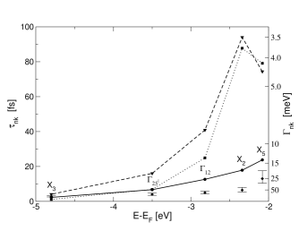
Figure 1: Lifetimes of selected d-bands of copper. Diamonds with error bars: experimental data from Ref. angel . The theoretical results obtained in this work are reported for different level of iterations within the the $G_{i}W_{0}$ quasiparticle approximation. Full line; $G_{0}W_{0}$. Dotted line: “on mass-shell” $G_{0}W_{0}$. Dashed line: “on mass-shell” $G_{1}W_{0}$. All theoretical quasiparticle energy position are aligned to the corresponding experimental values. For a comparison of the band positions see Tab. 1. The lifetimes are systematically above the experimental values, as expected for the contribution of higher–order electron–electron and residual phononic contributions.

	DFT	$G_{0}W_{0}$	$G_{1}W_{0}$	$G_{2}W_{0}$	Experiment
$\Gamma_{12}-\Gamma_{25^{\prime}}$	$0.91$	$0.60$	$0.38$	$0.23$	$0.81$
$X_{5}-X_{3}$	$3.23$	$2.49$	$1.99$	$1.65$	$2.79$
$X_{5}-X_{1}$	$3.70$	$2.90$	$2.31$	$1.92$	$3.17$
$L_{3}-L_{3}$	$1.58$	$1.26$	$1.03$	$0.90$	$1.37$
$L_{3}-L_{1}$	$3.72$	$2.83$	$2.13$	$1.65$	$2.91$
$L_{1}-L_{2^{\prime}}$	$5.40$	$4.76$	$4.78$	$3.77$	$4.95$

Table 1: Theoretical bandwidths (in eV) and band energies for copper, at high-symmetry points and for various iterations of the $G_{i}W_{0}$ quasiparticle approximation. There is a striking agreement with the experiment at the $G_{0}W_{0}$ level noi , but this worsens when the number of iterations is increased, showing the potential importance of including also vertex corrections. The experimental values are taken from ref. courths .

The proper inclusion of these non trivial self–energy corrections change the electronic decay channels of the d levels. In particular, we expect a strong effect on the topmost bands. Let us develop this idea further, by looking at the $G_{0}W_{0}$ expression for the self–energy:

$$\Sigma_{0}\left({\bf r}\,{\bf r}^{\prime},\omega\right)=\int\,\frac{i\,d\omega^{\prime}}{2\pi}G_{0}\left({\bf r}\,{\bf r}^{\prime},\omega^{\prime}\right)W_{0}\left({\bf r}\,{\bf r}^{\prime},\omega-\omega^{\prime}\right).$$ (6)

$W_{0}\left({\bf r},{\bf r}^{\prime};\omega^{\prime}\right)$ is the dynamically screened potential (convolution of the inverse dielectric function $\epsilon^{-1}\left({\bf r},{\bf r}^{\prime};\omega^{\prime}\right)$ with the bare Coulomb potential). We can write explicitly Eq. (3) in terms of a summation over the DFT states embodied in $G_{0}$ as:

$$\Gamma_{n{\bf k}}\propto\sum_{n^{\prime}}\sum_{\bf q}Im\left[W_{n{\bf k}\rightarrow n^{\prime}\left({\bf k-q}\right)}\left(\epsilon_{n^{\prime}\left({\bf k-q}\right)}^{DFT}-\epsilon_{n{\bf k}}^{QP,0}\right)\right]\\ \theta\left(\epsilon_{n^{\prime}\left({\bf k-q}\right)}^{DFT}-\epsilon_{n{\bf k}}^{QP,0}\right)f_{n^{\prime}\left({\bf k-q}\right)},$$ (7)

where

$$W_{n{\bf k}\rightarrow n^{\prime}\left({\bf k-q}\right)}\left(\omega\right)\equiv\int\,d{\bf r}d{\bf r}^{\prime}\psi^{*}_{n{\bf k}}\left({\bf r}\right)\psi_{n^{\prime}\left({\bf k-q}\right)}\left({\bf r}\right)\\ W\left({\bf r}\,{\bf r}^{\prime},\omega\right)\psi^{*}_{n^{\prime}\left({\bf k-q}\right)}\left({\bf r}^{\prime}\right)\psi_{n{\bf k}}\left({\bf r}^{\prime}\right),$$ (8)

being $f_{n{\bf k}}$ the Fermi occupations and $\theta\left(\omega\right)$ the step function. In Eq. (7) a quasihole in the state $|n{\bf k}\rangle$ looses energy via transitions to all the possible occupied states with (higher) energy $\epsilon_{n^{\prime}\left({\bf k-q}\right)}^{DFT}$; the energy difference is dissipated by the the screening cloud (described by $W\left(\omega\right)$) that surrounds the DFT hole $|n{\bf k}\rangle$. Thus the $G_{0}W_{0}$ transitions contributing to the hole linewidth look like single particle transitions from a quasihole to a DFT hole. In higher order of Hedin’s equations, i.e. including vertex corrections, this interpretation of transitions looses meaning. This is due to self–energy effects on the Green’s function of Eq. (6) and interactions of the screening cloud with the state $|n^{\prime}\left({\bf k-q}\right)\rangle$ (vertex corrections hedin ) that in Eq. (7) are neglected.

For the top of the occupied d bands the $G_{0}W_{0}$ calculation yields negative QP corrections noi ; this means that Eq. (7) contains also contributions coming from the decay of the QP d band to exactly the same DFT band. We will refer to these transitions as “intraband” decay channels. These contributions are important because the d–bands of copper are flat, hence the corresponding density of states is large. Moreover the screened interaction between d–bands is strong, as the d–states are spatially localized and screening is less effective at small distances. In the “on mass-shell” calculation the states $|n^{\prime}\left({\bf k-q}\right)\rangle$ appearing in Eq. (7) and the quasiparticle states correspond to the same DFT eigenvalues; this means that the “intraband” decay channels occur at zero energy, where the low–energy Drude tail of the dielectric function dominates (and hence the screened interaction is vanishing). This leads to the usual interpretation of the long calculated lifetimes at the d bands top as due to the fact that these d states can only decay to s/p states. These matrix elements are smaller than those involving states with the same l–character.

Even if the results of the $G_{0}W_{0}$ calculation are in rather good agreement with the experiments, a natural question about the physical meaning of the “intraband” decay channels arises. Being not at self-consistency, the system is described within $G_{0}W_{0}$ on the basis of quasiparticle states and DFT states (those involved in the hole decay) with different energies. To remove this inconsistency Eq. (1) should be solved iteratively, until converged QP energies are obtained. However, as we show below, iterations beyond the usual $G_{0}W_{0}$ level worsen both the imaginary and real parts of the calculated QP energies.

So far fully self-consistent $GW$ calculations have been performed only for the homogeneous electron gas holm and for simple semiconductors and metals eguiluz , yielding worse spectral properties than those obtained in the non self-consistent $G_{0}W_{0}$. The construction of a self-consistent $GW$ self–energy is a formidable task even for the simple systems mentioned above. In copper, already the update of the screening function is rather demanding, due to the presence of localized d orbitals that imply a large cut–off in the plane wave expansion. To test the effect of self-consistency on the QP energies and lifetimes we use a simplified $G_{i}W_{0}$ method, where the self–energy operator is defined as

$$\Sigma_{i}\left({\bf r}\,{\bf r}^{\prime},\omega\right)\equiv\int\frac{i\,d\omega^{\prime}}{2\pi}G_{i}\left({\bf r}\,{\bf r}^{\prime},\omega^{\prime}\right)W_{\left(0\right)}\left({\bf r}\,{\bf r}^{\prime},\omega-\omega^{\prime}\right),$$ (9)

being $i$ is the iteration number. $G_{i}$ involves the QP energies obtained from $\Sigma_{\left(i-1\right)}$, without considering renormalization factors, lifetimes, and energy structures beyond QP peaks. As the QP bandstructure resulting from the first iteration is already in excellent agreement with experiment, our next step is to perform an “on mass-shell” $G_{1}W_{0}$ calculation. The resulting lifetimes are compared with experiment in Fig.1. One sees that forcing QP energies to appear also in the states involved in Eq. (7), i.e. the states forward which the quasihole decays, yields lifetime results similar to those of the “on mass-shell” $G_{0}W_{0}$ method. The same overestimation of the lifetimes of the top of the d bands is observed, confirming that a good agreement with experiment depends on the inclusion of the “intraband” decay channels described by Eq. (7).

A further question could now be addressed and is how self-consistency affects the quasiparticle bandstructure obtained within $G_{0}W_{0}$. As shown in Tab. 1, at higher iteration orders of the quasiparticle $GW$ equation the resulting energies worsen. The d–bands width decreases, reducing the agreement with experiment.

These results show that $G_{0}W_{0}$ describes correctly the d–holes lifetimes as far as “intraband” decay channels between d–like states are included. Those transitions, however, imply an inconsistency between the quasiparticle initial states and the DFT final states of the hole decay, as shown in Eq. (7). A self–consistent solution of Dyson equation removes this inconsistency, worsening, however, the agreement with the experimental results. This is a clear indication of the need of including vertex corrections in the self–consistent procedure. As shown for simple metals shirley , vertex corrections would partially cancel the dressing of the $G_{0}$ Green’s function of Eq. (6), restoring the “intraband” decay channels and, consequently, the $G_{0}W_{0}$ results.

In conclusion, we have shown that the lifetimes of d–holes in copper, calculated within the $G_{0}W_{0}$ method, are in good agreement with the experimental results, and can be obtained within the very same scheme which yields a good quasiparticle bandstructure. In contrast, further iterations of the QP equation beyond the $G_{0}W_{0}$ level yield worse results, for both the real and imaginary parts of self–energy. This can be explained by the need of including also vertex corrections together with self–consistency. This result is quite general and should apply to all metals in which one has two or more sets of electronic states with different degrees of spatial localization.

This work has been supported by the INFM PRA project “1MESS”, MURST-COFIN 99, Basque Country University, Iberdrola S.A. and DGES. and by the EU through the NANOPHASE Research Training Network (Contract No. HPRN-CT-2000-00167). We thank F. Aryasetiawan and P.M. Echenique for helpfull discussions.

References

- (1) I. Campillo et al., Phys. Rev. Lett. 83, 2230 (1999); Phys. Rev. B 62, 1500 (2000).
- (2) V. P. Zhukov et al.,Phys. Rev. B 64, 195122 (2001).
- (3) V.M. Silkin et al., Phys. Rev. B 64, 085334 (2001); I. Campillo et al, Phys. Rev. B 61, 13484 (2000).
- (4) For a review, see P.M. Echenique, J.M. Pitarke, E.V. Chulkov and A. Rubio, Chem. Phys. 251, 1 (2000).
- (5) C.D. Spataru et al.,Phys. Rev. Lett. 87, 246405 (2001); G. Moos et al.,Phys. Rev. Lett. 87, 267402 (2001).
- (6) A. Gerlach et al., Phys. Rev. B 64, 085423 (2001); and references therein.
- (7) W. Kohn and L. J. Sham, Phys. Rev. 140, A1113 (1965); P. Hohenberg and W. Kohn, Phys. Rev. 136, B864 (1964).
- (8) For a review, see Recent Advances in Density Functional Methods, (World Scientific, Singapore, 2002 and 1995).
- (9) D.M. Ceperley and B.J. Alder, Phys. Rev. Lett. 45, 566 (1980); J. P. Perdew and A. Zunger, Phys. Rev. B 23, 5048 (1981).
- (10) A. Marini, R. Del Sole, G. Onida, Phys. Rev. Lett. 88, 016403 (2002).
- (11) For a review, see G. Onida, L. Reining and A. Rubio, Rev. Mod. Phys. 74, 601 (2002).
- (12) L. Hedin, Phys. Rev. 139, A796 (1965).
- (13) I. Campillo et al., Phys. Rev. Lett. 85, 3241 (2000).
- (14) F. Aryasetiawan and O. Gunnarsson, Rep. Prog. Phys. 61, 237-312 (1998).
- (15) J.J. Quinn and R.A. Ferrell, Phys. Rev. 112, 812 (1958).
- (16) N. Troullier and J.L. Martins, Phys. Rev. B 43, 1993 (1991).
- (17) A. Marini, R. Del Sole, G. Onida, Phys. Rev. B 64, 195125 (2001).
- (18) The screened interaction has been calculated inverting, in the reciprocal space, a dielectric matrix. The corresponding polarization function has been integrated using a uniform grid of 256 q–points together with a set of 1000 random k–points (in the whole Brillouin zone). The above set of G,q and k vectors ensure a convergence of the results within 5%.
- (19) R. Courths and S. Hüfner, Phys. Rep. 112, 53 (1984).
- (20) U.V. Barth and B. Holm, Phys. Rev. B 54,8411 (1996).
- (21) W.D. Schöne and A.G. Eguiluz, Phys. Rev. Lett. 81, 1662 (1998).
- (22) E. L. Shirley, Phys. Rev. B 54,7758 (1996).