Selective advantage of topological disorder in biological evolution

Abstract

We examine a model of biological evolution of Eigen’s quasispecies in a so-called holey fitness landscape, where the fitness of a site is either $0$ (lethal site) or a uniform positive constant (viable site). The evolution dynamics is therefore determined by the topology of the genome space which is modelled by the random Bethe lattice. We use the effective medium and single-defect approximations to find the criteria under which the localized quasispecies cloud is created. We find that shorter genomes, which are more robust to random mutations than average, represent a selective advantage which we call “topological”. A way of assessing empirically the relative importance of reproductive success and topological advantage is suggested.

1 Introduction

The mechanism of biological evolution is a very challenging topic for the physical community. This is well expressed in the numerous models of biological evolution that have emerged in recent years. The list of models studied starts with large-scale properties of the evolutionary process—massive global extinctions—and ends with the works which are aimed at following the replicative behavior of the chemical structures holding information, namely DNA molecules. A lot of effort has been devoted to this area recently ba_fly_la_92 ; ba_sne_93 ; pa_ma_ba_96 ; va_au_95 ; fe_pla_dia_95 ; so_ma_96 ; ro_ne_96 ; zhang_97 ; drossel_98 ; sol99 ; sla_kot_99 ; sla_kot_00 ; kot_sla_sta_02 ; nim_cru_huy_99 ; wilke_01 ; wilke_01a and still new fruitful ideas emerge kra01 ; chri_coll_hall_jen02 ; hall_chri_coll_jen02 .

The process of biological evolution consists in three steps: $reproduction\rightarrow mutation\rightarrow selection.$ The important thing to note is that the biological fitness function which denotes an individuals’ ability to produce viable offsprings depends on their phenotype. On the other hand, the mutations occur in the genotype—information stored in a sequence of DNA. The fitness function, which assigns to each microscopic genotype its ability to reproduce and pass on to the next generation, shows an overwhelming complexity. This property makes the theoretical treatment of evolution an extremely complicated task.

Simplifications of the problem are necessary. The fruitful idea of adaptive landscapes was introduced by Wright wri31 and was later further simplified to fitness landscapes later. In this scheme the individual is represented as a point in a multidimensional space and to every point a fitness value is assigned. Thus, a landscape is formed of mountains of genetically adapted positions and valleys of lethal genomes. Note the idealization: the fitness is directly given by the genome of the individual, not by its (extended) phenotype.

In fact, the fitness landscape is not static since it strongly depends on the ever changing environment, which includes interactions with (co)evolving species as well as abiotic influences kauffman_90a ; kau91 ; wil01 . Evolutionary process manifests itself the ascent of individuals to peaks on the fitness landscape.

A broad set of different fitness landscapes was recently used to study the behavior of the evolutionary system. These models employ both static pel01 ; alt01 and dynamic landscapes wil01 ; nil00 ; pekalski_00 ; pek_wer_01 . They include the sharply-peaked landscape (SPL) with a single preferred genome (wildtype), the Fujiyama landscape, or the holey landscape (HL). Several recent reviews summarize various approaches explored wil01 ; baa99 ; pel97 ; drossel_01 .

Generally, one simplifies the genetic code considering only a two-letter $\{0,1\}$ alphabet. Let us consider, for example, the digits $1$ and $0$ as symbols for two different alleles of a certain gene. Assuming constant genome length of $d$ loci the state space is a hypercube ${\mathcal{G}}=\{0,1\}^{d}$.

The dynamics of evolution on fitness landscapes have the most prominent scheme in the quasispecies model as introduced by Eigen eig71 . Originally it was introduced as a model for chemical prebiotic evolution, but it showed itself plausible in the investigation of the mechanisms of microevolution of viruses and bacteria, i.e. organisms with relatively simple genomes.

The quasispecies is defined as a cloud of closely related individuals. They hang together but certainly they may move on the fitness landscape. We assume an infinite population size and therefore the dynamics of the quasispecies are probabilistic, but without any noise which would be induced by finite size effects. The quasispecies obeys three basic processes: reproduction, selection and is liable to mutational genetic changes. Reproduction and selection are treated together—the reproductive ability depends on the fitness and hence selection takes part here. Mutation can occur in the individual’s genome with a probability rate $\mu$.

It is evident that the native geometry of the genome space is the above mentioned hypercube ${\mathcal{G}}=\{0,1\}^{d}$. So, this is the natural starting point when building a model for a fitness landscape. Recently, the main focus has been aimed at the presence or absence of the adaptive regime induced by a single maximum in the fitness landscape. Therefore, the first thing to try is the sharply-peaked landscape on the hypercube. This model was solved exactly by Galluccio et al. ga_gra_zha_96 ; galluccio_97 .

The most important feature found in the quasispecies model in SPL is the error threshold tar92 ; fra97 . It is the phase transition that separates two regimes of the quasispecies evolution, namely the adaptive regime and the wandering regime. In the adaptive regime the localized cloud of quasispecies is formed around the wildtype (for us a certain site in the lattice), whereas in the wandering regime no quasispecies is formed due to a mutation load.

The error threshold phenomenon comes out of the competition between the selective advantage of a certain wildtype and the mutation load presented by the rate $\mu$. The threshold is then characterized by the specific value of the selective advantage. We want to show that the selective advantage in the specific site is not the only parameter, whose value can distinguish two significantly different regimes. There are also geometrical properties, e.g. connectivity of the site, that can make the genotype in the specific site advantageous. These are the main tasks of this article.

Indeed, the real landscapes are far more complicated than SPL. It is expected that rugged landscapes with many competing maxima represent a realistic picture ba_fly_la_92 . Such landscapes are well-known in the theory of spin glasses me_pa_vi_87 and a “spin-glass” theory of evolution was investigated, e.g. in am_pe_sa_91 . In our previous work we have studied several similar models of the fitness landscape, too kol_sla_02 .

Yet another approach to the modelling of the fitness landscape is used for computations gav98 ; gav99 —the so-called holey landscape (HL), where the fitness is either a positive constant (which may be set to $1$) or it is $0$ which means that the individual with the corresponding genetic code dies with a probability of $1$ without having offspring.

Indeed, a large part of the point mutations which may occur at the basic level of the evolutionary picture are lethal for the individual—they lead to the ‘lethal’ sites. Therefore, the hypercube does not represent a good approximation to the evolutionary dynamics, because only a small part of its edges represent paths to possible new ‘hospitable’ genomes.

A sparsely connected set of points selected at some of the hypercube corners is perhaps a better choice. Such sparse graphs and their adjacency matrices are under study extensively at present; see e.g. bi_mo_99 ; monasson_99 ; sem_cug_02 and references therein. The authors observe the localization of the eigenvectors of the sparse matrices due to topological characteristics only.

We approach the problem from a somewhat different perspective which resembles the study of topologically disordered solids where the random network of bonds is often well modelled by the Bethe lattice wil_mas_vel_86 . This, of course, supposes that there are no short loops in the graph. Supposing we are above the percolation threshold, our random lattice forms a giant cluster within the hypercube and the typical length of loops is in the number of sites $N=2^{d}$ of order $\log N$, where $N$ is the total number of sites $N=2^{d}$, see bollobas_85 . Thus, the Bethe lattice may be a good model for the topology of our sparse graph.

The main question addressed in our work will be the following: Selective advantage in biological evolution is usually attributed to higher reproductive success. If advantage due to high individual fitness exceeds a certain threshold, a quasispecies is formed around the site. This is the usual error-threshold phenomenon. Here we ask, whether some factors related purely to the structure or topology of the genome space may lead to similar selective advantage, and if a certain threshold can be found separating the adaptive and wandering regime of biological evolution.

2 Model

Recently, kol_sla_02 we have modelled evolution in a holey landscape using the regular Bethe lattice. Now we will try to represent it in a more precise way and take into account the irregularity of the lattice. For each site we select whether the links that leave it lead to another ‘hospitable’ site of the hypercube, or not. In the latter case, there are some links leading from the site to the ‘lethal’ sites of the hypercube and so all mutants that took this direction are doomed.

We start with a regular Bethe lattice with a connectivity $k$. We construct the irregular Bethe lattice by randomly assigning lethal sites and removing all sites which are connected to the rest of the lattice only through a lethal site. The evolution process amounts to diffusion on this lattice. Hops from a viable site to any of its neighbors occur with an equal rate $\mu$. Hops from lethal sites are prohibited. So, the edges to lethal sites are “dead ends” or “dangling bonds”, in the language of condensed matter physics.

Let $i$ be a viable site. Let us denote $(i)$ as the set of viable neighbors of $i$. $\kappa_{i}=|(i)|\leq k$ is the number of those viable neighbors. For $k$ we suppose only that it is large enough to fulfill the previous inequality. The arbitrariness of the choice of $k$ will be clarified later on. Intuitively, during evolution the probability will flow out from $i$ to all its $k$ neighbors, but flow in only from $\kappa_{i}$ viable ones. Therefore, we expect that a site with larger $\kappa_{i}$ is more likely to gather individuals and form a quasispecies cloud. The scope of this paper is to elaborate this intuitive picture in a more formal manner.

If we denote $p_{i}(t)$ as a (relative) population of site $i$ at time $t$, we can write the following master equation

$$\dot{p}_{i}(t)=\sum_{j}T_{ij}\,p_{j}(t)$$ (1)

where the matrix $T$ contains the effects of mutations and reproduction:

$$T_{ij}=\left\{\quad\begin{array}[]{rl}-\mu\,k+\zeta&i=j\\ \mu&j\in(i)\\ 0&\text{elsewhere.}\end{array}\right.$$ (2)

The constant $\zeta$ is introduced artificially in order to keep the total population constant. In fact, there are two causes of the net population outflow which must be countered by the $\zeta$ term. The first one is the presence of traps—lethal sites that absorb the individuals. The second one comes from the very topology of the Bethe lattice. Indeed, any finite Bethe lattice has the rather counter-intuitive property that the number of the surface sites is comparable to the number of bulk sites and this property holds even in the limit of an infinite number of sites. Therefore, there is always a net flow of probability toward the surface. However, we are interested in the properties of the sites deep in the bulk and the outflow toward the surface should be considered as an artifact of the Bethe lattice approximation. To sum up, we will fix the value of $\zeta$ later on in the calculations, in order that the population remains fixed.

The dynamical matrix $T$ is in the model symmetric, and this enables us to use the method of the resolvent in our calculations. The symmetry results from the assumption of equal mutation rates, $\mu$. This widely used approximation simplifies all the following calculations and, since we are interested only in a stationary state of the system, it is not considered to change the main results. One can introduce the edge-dependent rates $\mu_{ij}$ and then $\zeta$ would become a function of all $p_{i}(t)$ and Eq. (1) would generally become non-linear one. But this approach goes beyond the scope of our article.

3 Partitioning

As in the previous paper kol_sla_02 we investigate the formation of a localized state, now interpreted as a quasispecies cloud, through the properties of the resolvent of the matrix $T$

$$\mathcal{G}(z)=(z-T)^{-1}\;.$$ (3)

The idea of the calculation is quite simple: In the long-time limit only the largest eigenvalue of the matrix $T$ survives, and the corresponding eigenvector describes the stationary state of the evolutionary system.

In order to find the largest eigenvalue of $T$, we search for the poles of an element of the resolvent matrix $\mathcal{G}$. These are exactly the eigenvalues of $T$, no matter which element of $\mathcal{G}$ we choose. And since we want to observe the formation of the localized state around a specific site $i=1$, we need the diagonal matrix element of the resolvent

$$G(z)=[\mathcal{G}(z)]_{11}$$ (4)

which can be calculated using the partitioning (projector) method lowdin_62 , explained in more detail in kol_sla_02 . The loop-less structure of the Bethe lattice greatly simplifies the treatment. We proceed essentially in two steps, which are illustrated in the Fig. 1. In the first step, we project out of the site $i=1$ itself. The rest of the Bethe lattice splits into disconnected branches. We find

$$G(z)=\frac{1}{z+\mu k-\zeta-\mu^{2}\sum_{j\in(1)}\Gamma_{j}(z)},$$ (5)

where $\Gamma_{j}(z)$ is the diagonal element of the projected resolvent on the terminal site of the branch starting with site $j$. (The terminal sites are denoted as $2$ in Fig. 1.)

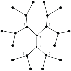
Figure 1: Division of the Bethe lattice during the partitioning.

In the second step, we calculate $\Gamma_{j}(z)$ by projecting out the site $j$. We find, similar to the previous case,

$$\Gamma_{j}(z)=\frac{1}{z+\mu k-\zeta-\mu^{2}\sum_{l\in(j)\backslash\{1\}}\Gamma_{l}(z)}\;.$$ (6)

Some of the sites $l\in(j)\backslash\{1\}$ are denoted by $3$ in Fig. 1. Iterating the equation (6) we could in principle calculate the resolvents on the terminal sites and inserting them into Eq. (5) obtain the desired quantity.

This procedure works well in an infinite regular Bethe lattice, where $\Gamma_{j}(z)$ for $j$ deep in the bulk does not depend on the site index $j$ and (6) represents in fact a closed equation for $\Gamma(z)\equiv\Gamma_{j}(z)\;\forall j$. However, this procedure cannot be directly applied in the case of an irregular Bethe lattice. Nevertheless, it is a good starting point for an approximation we will describe in the following.

4 Effective medium approximation

The mean-field-type treatment of disordered solids was developed a long time ago within the coherent potential approximation (CPA) vel_kir_ehr_68 . In the theory of sparse random matrices it was elaborated using the replica method bi_mo_99 ; monasson_99 ; sem_cug_02 and called the effective medium approximation (EMA). In this section we will use the EMA for the irregular Bethe lattice without using the replica trick.

The main idea relies on a simple observation that the sum $\sum_{l\in(j)\backslash\{1\}}\Gamma_{l}(z)$ containing $\kappa_{j}-1$ terms can be replaced by its average value for large $\kappa_{j}$, thus neglecting fluctuations. Indeed, it was proved that the CPA is exact in the limit of infinite connectivity jan_vol_92 . Therefore, our version of the EMA amounts to approximating

$$\sum_{l\in(j)\backslash\{1\}}\Gamma_{l}(z)\simeq(\kappa_{j}-1)\,\langle\Gamma(z)\rangle\;.$$ (7)

In order to close the equations, we must average expression (6) over the probability distribution of connectivities $P(\kappa)$

$$\langle\Gamma(z)\rangle=\sum_{\kappa}\frac{P(\kappa)}{z+\mu k-\zeta-\mu^{2}(\kappa-1)\langle\Gamma(z)\rangle}\;.$$ (8)

The latter equation (8) is the core of the EMA. When we insert its solution $\langle\Gamma(z)\rangle$ into (5) and perform again the average over connectivities, we obtain the averaged diagonal element of the resolvent $\langle G(z)\rangle$, which is now site-independent. The parameter $\zeta$ represents the shift in the variable $z$ and should be adjusted so that the upper edge of the support of the imaginary part of $\langle G(z)\rangle$ (i.e. the density of states) lies at $z=0$. This expresses the requirement of the conservation of the population size.

Figure 2: The averaged resolvent at terminal site $\langle\Gamma(z)\rangle$ for the irregular Bethe lattice with connectivity distribution defined in (9), where $p=\frac{1}{2}$. Full line: imaginary part. Dashed line: real part.

As an illustration we show in Fig. 2 the real and imaginary parts of $\langle\Gamma(z)\rangle$ for the connectivity distribution chosen as

$$P(\kappa)=p\,\delta(\kappa-2)+(1-p)\,\delta(\kappa-3)$$ (9)

for $0\leq p\leq 1$. We can see that the imaginary part of $\langle\Gamma(z)\rangle$ approaches zero as $z^{1/2}$ at the band edge and the real part approaches a finite limit. From the technical point of view, the finiteness of the limit is the source of the transition between localized and delocalized states.

5 Single defect

So far we have investigated the Bethe lattice as an averaged homogeneous effective medium. Now we investigate the behavior of the resolvent at a site $i=1$ with a specific connectivity $\kappa_{1}$. The situation is schematically depicted in Fig. 3.

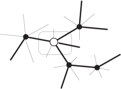
Figure 3: The “defect” site with a different connectivity. Thin links represent lethal mutations, the thick ones mutations to viable sites.

This approach has a biological motivation. What we see in nature is that there are frequent groups of closely related animals. These groups form taxonomic classes or, better said, the classes are defined as the groups of such closely related individuals. In the following, we examine if the clustering of individuals, modelled as the addition of the site with largest connectivity, leads to some observable changes in the quasispecies evolutionary process.

The on-site resolvent corresponding to this site can be found from Eq. (5), where the resolvents at the terminal sites are approximated as in (7). This is the essence of the single-defect approximation (SDA). Hence

$$G_{\rm SDA}(z)=\frac{1}{z+\mu k-\zeta-\mu^{2}\kappa_{1}\langle\Gamma(z)\rangle}\;.$$ (10)

A state localized at this site exists, if the resolvent $G_{\rm SDA}(z)$ has a pole for a real positive $z$. This is equivalent to the condition

$$\kappa_{1}>\kappa_{c}\equiv\frac{\mu k-\zeta}{\mu^{2}}\,\frac{1}{{\rm Re}\langle\Gamma(0)\rangle}\;.$$ (11)

Therefore, the state is localized and the quasispecies cloud is formed for integer $\kappa_{1}$ greater than $\kappa_{c}$. This corresponds to the adaptive regime of the evolutionary process. We use as an example again the distribution (9) and show in the Fig. 4 the dependence of the threshold $\kappa_{c}$ on the parameter $p$ of the probability distribution.

Figure 4: The dependence of the critical value of the connectivity, $\kappa_{c}$, on $p$, for connectivity distribution (9).

We will consider yet another type of “defect” in the effective medium. Imagine that the site investigated, $i=1$, corresponds to a genome of length different to the average. This difference is translated in our model as a choice of different total connectivity $k$ in the site $i$ (including edges to both viable and lethal sites). So, we may replace $k\to k+\lambda$ in Eq. (10). Then we may investigate the transition from the wandering to the adaptive regime when varying two parameters $\lambda$ and $\kappa_{1}$. We will see that the individuals added due to the $\zeta$ term in Eq. (1) are redistributed in the lattice in such a manner that the total population changes. This is only due to addition of the “defect” and the localization of individuals in its vicinity. The condition for the existence of a localized state, i.e. for the adaptive regime, is analogous to (11) and can be written as

$$\lambda<\lambda_{c}\equiv\mu\kappa_{1}\,{\rm Re}\langle\Gamma(0)\rangle-\frac{\mu k-\zeta}{\mu}\;.$$ (12)

Figure 5: The dependence of the critical value $\lambda_{c}$ on the probability $p$, for distribution (9) and $\kappa_{1}=5$.

We show in Fig. 5 an example of the dependence of $\lambda_{c}$ for the same connectivity distribution (9) as in previous cases, and for a specific, fixed choice of $\kappa_{1}$.

6 Conclusions

We modelled the complex fitness landscape of biological evolution with an irregular Bethe lattice. The formation of localized quasispecies in the adaptive regime was observed via the occurrence of the isolated pole in the on-site resolvent. Using the effective medium approximation we calculated the disorder-averaged resolvent and within the single-defect approximation we investigated the localization.

We found that the quasispecies is formed if the site is connected to a sufficiently large number of viable sites. We found the condition for the critical value of the connectivity $\kappa_{c}$ separating the adaptive evolutionary regime for $\kappa>\kappa_{c}$ and the wandering regime for $\kappa<\kappa_{c}$. As expected, $\kappa_{c}$ grows with the average connectivity and qualitatively speaking the quasispecies are formed at such sites that have sufficiently larger number of viable neighbors than average. We may interpret it as a purely topological selective advantage: The species has better chance to survive not because of its individual reproductive abilities, but because it is less vulnerable to random alterations of the genetic code.

We investigated also another deviation from the mean, connected to the overall number of neighbors. In more biological language it corresponds to the length of the genetic code. We observed that the adaptive regime is favored for lower values of the connectivity, i.e. for shorter genomes, if the number of viable neighbour sites is considered constant. This type of selective advantage is therefore also of topological origin and has a similar biological interpretation to that presented above. Indeed, longer genome means higher probability of a lethal mutation.

In both cases it is important to note that it is the deviation from the average topology which makes the selective advantage work and which leads to the formation of localized states. So, it is the (sufficiently strong) topological disorder that is responsible for the formation of quasispecies.

We may conclude by summarizing that without resort to individual reproductive capacities, biological evolution favors genomes which are shorter and more robust to random mutations. This has one more important implication; a genome, which can be easily mutated without affecting the death of its carrier, means also a less-defined species. One may therefore predict that successful species will exist in a broad variety of slightly different sub-species. This effect is caused by the selective advantage of certain topologies of the genome space. Observation of the variability within a single species may therefore say something of the relative importance of topological selective advantage in comparison to individual reproductive success.

- (1) P. Bak, H. Flyvbjerg and B. Lautrup, Phys. Rev. A 46, 6724 (1992).
- (2) P. Bak and K. Sneppen, Phys. Rev. Lett. 71, 4083 (1993).
- (3) M. Paczuski, S. Maslov and P. Bak, Phys. Rev. E 53, 414 (1996).
- (4) N. Vandewalle and M. Ausloos, J. Phys. I France 5, 1011 (1995).
- (5) J. Fernandez, A. Plastino, and L. Diambra, Phys. Rev. E 52, 5700 (1995).
- (6) R. V. Solé and S. C. Manrubia, Phys. Rev. E 54, R42 (1996).
- (7) B. W. Roberts and M. E. J. Newman, J. Theor. Biol 180, 39 (1996).
- (8) Y.-C. Zhang, Phys. Rev. E 55, R3817 (1997).
- (9) Barbara Drossel, Phys. Rev. Lett. 81, 5011 (1998).
- (10) R. V. Sole, R. Ferrer, I. Gonzalez–Garcia, J. Quer, and E. Domingo, J. Theor. Biol. 198, 47 (1999).
- (11) F. Slanina and M. Kotrla, Phys. Rev. Lett. 83, 5587 (1999).
- (12) F. Slanina and M. Kotrla, Phys. Rev. E 62, 6170 (2000).
- (13) M. Kotrla, F. Slanina, and J. Steiner, Europhys. Lett. 60, 14 (2002).
- (14) E. van Nimwegen, J. P. Crutchfield, and M. Huynen, Proc. Natl. Acad. Sci. USA 96, 9716 (1999).
- (15) C. O. Wilke, Bull. Math. Biol. 63, 715 (2001).
- (16) C. O. Wilke, Evolution, 55, 2412 (2001).
- (17) P. Král, J. Theor. Biol. 212, 355 (2001).
- (18) K. Christensen, S. A. di Collobiano, M. Hall, and H. Jensen, J. Theor. Biol. 216, 73 (2002)
- (19) M. Hall, K. Christensen, S. A. di Collobiano, and H. Jensen, Phys. Rev. E 66, 011904 (2002).
- (20) S. Wright, Genetics 16, 97 (1931).
- (21) S. A. Kauffman, The Origins of Order: Self-organization and Selection in Evolution (Oxford University Press, Oxford, 1993).
- (22) S. A. Kauffman and S. Johnson, J. Theor. Biol. 149, 467 (1991).
- (23) C. O. Wilke, C. Ronnewinkel and T. Martinetz, Phys. Rep. 349, 395 (2001).
- (24) L. Peliti, Europhys. Lett. 57, 745 (2002).
- (25) S. Altmeyer and J. S. McCaskill, Phys. Rev. Lett. 86, 5819 (2001).
- (26) M. Nilsson, Phys. Rev. Lett. 84, 191 (2000).
- (27) A. Pekalski, Eur. Phys. J. B 17, 329 (2000).
- (28) A. Pekalski and K. Sznajd–Weron, Phys. Rev. E 63, 031903 (2001).
- (29) E. Baake and W. Gabriel, Ann. Rev. Comp. Phys. VII ed. D. Stauffer, pp. 203-264 (World Scientific, Singapore, 2000); cond-mat/9907372.
- (30) L. Peliti, cond-mat/9712027.
- (31) B. Drossel, Adv. Phys. 50, 209 (2001).
- (32) M. Eigen, Naturwissenschaften 58, 465 (1971).
- (33) S. Galluccio, R. Graber, and Y.-C. Zhang, J. Phys. A: Math. Gen. 29, L249 (1996).
- (34) S. Galluccio, Phys. Rev. E 56, 4526 (1997).
- (35) P. Tarazona, Phys. Rev. A 45, 6038 (1992).
- (36) S. Franz, L. Peliti J. Phys. A: Math. Gen 30, 4481 (1997).
- (37) M. Mézard, G. Parisi, and M. A. Virasoro, Spin Glass Theory and Beyond , (World Scientific, Singapore 1987).
- (38) C. Amitrano, L. Peliti, and M. Saber, in: Molecular Evolution on Rugged Landscapes, ed. A. Perelson and S. Kauffman, p. 27 (Addison-Wesley 1991).
- (39) M. Kolář and F. Slanina, Physica A, 313, 549 (2002).
- (40) S. Gavrilets, H. Li, M.D. Vose, Proc. R. Soc. Lond. B 265, 1483 (1998).
- (41) S. Gavrilets, American Naturalist 154, 1 (1999).
- (42) G. Biroli and R. Monasson, J. Phys. A: Math. Gen. 32, L255 (1999).
- (43) R. Monasson, Eur. Phys. J. B 12, 555 (1999).
- (44) G. Semerjian and L. F. Cugliandolo, J. Phys. A 35, 4837 (2002).
- (45) S. Wilke, J. Mašek, and B. Velický, Phys. Stat. Sol. (b) 135, 309 (1986).
- (46) B. Bollobás, Random Graphs (Academic Press, London, 1985).
- (47) P.-O. Löwdin, J. Appl. Phys. (Suppl.) 33, 251 (1962).
- (48) B. Velický, S. Kirkpatrick, and H. Ehrenreich, Phys. Rev. 175, 747 (1968).
- (49) V. Janiš and D. Vollhardt, Phys. Rev. B 46, 15712 (1992).