Semi–analytical solution of the Kondo model in a magnetic field

Abstract

The single impurity Kondo model at zero temperature in a magnetic field is solved by a semi–analytical approach based on the flow equation method. The resulting problem is shown to be equivalent to a resonant level model with a non–constant hybridization function. This nontrivial effective hybridization function encodes the quasiparticle interaction in the Kondo limit, while the magnetic field enters as the impurity orbital energy. The evaluation of static and dynamic quantities of the strong–coupling Kondo model becomes very simple in this effective model. We present results for thermodynamic quantities and the dynamical spin–structure factor and compare them with NRG calculations.

I Introduction

The single impurity Kondo or $s$–$d$ model (SIKM) kondo

$$H_{\rm SIKM}=\sum\limits_{\vec{k}\sigma}\epsilon^{\phantom{\dagger}}_{\vec{k}}c^{\dagger}_{\vec{k}\sigma}c^{\phantom{\dagger}}_{\vec{k}\sigma}+J\sum\limits_{\vec{k}\vec{k}^{\prime}}\sum\limits_{\alpha\beta}c^{\dagger}_{\vec{k}\alpha}\,{\vec{S}}\cdot\vec{\sigma}^{\phantom{\dagger}}_{\alpha\beta}\,c^{\phantom{\dagger}}_{\vec{k}^{\prime}\beta}$$ (1)

is, together with its close relative, the single impurity Anderson model (SIAM) anderson , one of the fundamental models in the theory of correlated electron systems. It has been studied extensively over the past four decades hewson , but despite its simplicity, no complete analytic solution exists that provides information on both thermodynamic and dynamical quantities. For example, the Bethe ansatz solution bethe ; hewson has solved all universal properties of the Kondo problem including its high– to low–temperature crossover behavior. But the Bethe ansatz requires the limit of infinite conduction band width and cannot be used to calculate dynamical quantities beyond the low–energy limit.

Thus, numerical methods, like Wilson’s numerical renormalization group (NRG) Wilson ; hewson or quantum Monte–Carlo (QMC) fye , in connection with maximum–entropy methods MEM have to be employed to access dynamical quantities on all energy scales. In both methods, evaluation of dynamical properties, and quantities related to them, like the Korringa–Shiba relation or the Friedel sum rule hewson , suffer from unavoidable numerical errors. QMC simulations, in addition, cannot be used at zero temperature and are restricted to comparatively large values of $J$.fye Moreover, a reliable evaluation of single– and two–particle spectra and related quantities in an external magnetic field, as well as their comparison and interpretation within a local Fermi liquid picture hewson become rather problematic costi ; logan4 , especially in the limit of vanishing external magnetic field. Approximate analytical techniques, like perturbation expansions or $1/N$–expansions hewson , typically only describe certain properties of the Kondo model correctly. A notable exception in this respect is the so–called local moment approach (LMA) logan . This perturbative approach is very accurate in most cases logan2 , including those of nonvanishing external magnetic fields.logan3 ; logan4

Besides its relevance for the study of moment formation in metals, the SIKM (1) has gained new importance as input for investigating non–dilute correlated electron systems like heavy fermion materials within dynamical mean–field theory (DMFT).DMFT Here a reliable method for calculating single–particle correlation functions, especially close to the Fermi energy, is extremely important.

In this paper, we propose a new non–perturbative semi–analytical approach to the Kondo problem based on Wegner’s flow equation method wegner and previous work on applications of flow equations to strong–coupling problems strong_coupling ; Hofstetter_Kehrein . We will show that to a very good approximation, many physical quantities of the Kondo model can be calculated from a resonant level model (RLM), where the interacting features of the Kondo model are encoded in a non–constant effective hybridization function of this resonant level model. Surprisingly, this noninteracting effective model describes both universal low–energy properties like the Wilson ratio as well as high–energy power laws and logarithmic corrections with very good accuracy. Due to the noninteracting nature of this effective model this mapping allows immediate insights into the physics of the SIKM, for example the dependence of its static and dynamical quantities on a local magnetic field.

After presenting our approach in the next section, we will discuss several static quantities at $T=0$ as a function of a local magnetic field and derive analytical expressions for their asymptotic behavior. As an example for a dynamical quantity, we will then discuss the spin–structure factor and the Korringa–Shiba relation. An outlook on potential future applications of our approach concludes this paper.

II Mapping to a resonant level model

II.1 Principles of the flow-equation method

The general framework of the flow equation methodwegner and its application to the Kondo model has been explained in detail in Ref. Hofstetter_Kehrein, . Here we will only repeat the main steps in order to make this paper self–contained, and refer to Ref. Hofstetter_Kehrein, for more details.

The key idea of the flow equation approach consists in performing a continuous sequence of infinitesimal unitary transformations on a given Hamiltonian

$$\frac{dH(B)}{dB}=[\eta(B),H(B)]\ .$$ (2)

With an anti–Hermitian generator $\eta(B)$ the solution of equation (2) describes a family of unitarily equivalent Hamiltonians $H(B)$ parameterized by the flow parameter $B$. By choosing $\eta(B)$ appropriatelywegner one can set up a framework that diagonalizes a many–particle Hamiltonian $H(B=0)$, i.e. $H(B=\infty)$ becomes diagonal.

The concrete realization of this approach for the Kondo model was discussed in Ref. Hofstetter_Kehrein, . The starting point is the bosonized formboson of the Hamiltonian (1). Since we will be mainly interested in describing the basic ideas of our approach, we restrict ourselves to a linear dispersion relation. Notice, however, that the flow equation approach can also be used for a nontrivial conduction band density of states as it does not rely on the integrability of the model.perspective With a linear dispersion relation the Kondo problem becomes effectively one–dimensional, the charge density excitations in (1) decouple, and we only need to look at the spin density part

$$H=H_{0}-\frac{J}{\sqrt{8\pi^{2}}}\partial_{x}\Phi(0)\,S^{z}+\frac{J}{4\pi a}\,\left(e^{i\sqrt{2}\Phi(0)}\,S^{-}+{\rm h.c.}\right)$$ (3)

with $H_{0}=\sum_{q>0}q\,\sigma(q)\,\sigma(-q)$. Here $\sigma(p)=\frac{1}{\sqrt{2|p|}}\sum_{q}(c^{\dagger}_{p+q\uparrow}c^{\phantom{\dagger}}_{q\uparrow}-c^{\dagger}_{p+q\downarrow}c^{\phantom{\dagger}}_{q\downarrow})$ are the bosonic spin density modes with the bosonic spin density field defined by $\Phi(x)=-i\sum_{q\neq 0}\frac{\sqrt{|q|}}{q}\>e^{-iqx-a|q|/2}\>\sigma(q)$. For simplicity we have set the Fermi velocity $v_{F}=1$. $a$ is proportional to the inverse conduction band width. All our latter results will be expressed as universal functions of the low–energy Kondo scale $T_{\rm K}$, and we can consider (3) to be equivalent to our original Kondo Hamiltonian if $T_{\rm K}\ll a^{-1}$.

Eq. (3) was used as the starting point $H(B=0)$ of the flow equation approach in Ref. Hofstetter_Kehrein, . Away from the Toulouse point the unitary equivalence of the flow holds only approximately, but this approximation can be controlled by a small parameterstrong_coupling and yields very accurate results. During the flow the Hamiltonian can be parameterized as

$$H(B) = H_{0}+\sum_{p}g_{p}(B)\,\left(C^{\dagger}_{p}(\lambda(B))\,S^{-}+{\rm h.c.}\right)$$

$$+\sum_{p}\omega_{p}(B)\,\left[C^{\dagger}_{p}(\lambda(B_{p})),C^{\phantom{\dagger}}_{p}(\lambda(B_{p}))\right]\ .$$

Here $B_{p}\stackrel{{\scriptstyle\rm def}}{{=}}p^{-2}$, and $C^{\dagger}_{p}(\lambda),~{}C^{\phantom{\dagger}}_{p}(\lambda)$ denote normalized vertex operators with scaling dimension $\lambda>0$ in momentum space,

$$C^{\dagger}_{p}(\lambda) \stackrel{{\scriptstyle\rm def}}{{=}} \left(\frac{\Gamma(\lambda^{2})}{2\pi a\,L}\right)^{1/2}|pa|^{(1-\lambda^{2})/2}\int_{-L/2}^{L/2}dx\,e^{ipx+i\lambda\Phi(x)}$$

$$C^{\phantom{\dagger}}_{p}(\lambda) \stackrel{{\scriptstyle\rm def}}{{=}} \left(\frac{\Gamma(\lambda^{2})}{2\pi a\,L}\right)^{1/2}|pa|^{(1-\lambda^{2})/2}\int_{-L/2}^{L/2}dx\,e^{-ipx-i\lambda\Phi(x)}$$

that obey $\langle\Omega|C^{\phantom{\dagger}}_{p}(\lambda)\,C^{\dagger}_{p^{\prime}}(\lambda)|\Omega\rangle=\delta_{pp^{\prime}}\theta(p)$ and $\langle\Omega|C^{\dagger}_{p}(\lambda)\,C^{\phantom{\dagger}}_{p^{\prime}}(\lambda)|\Omega\rangle=\delta_{pp^{\prime}}\theta(-p)$. For the special case $\lambda=1$ they fulfill fermionic anticommutation relations $\{C^{\dagger}_{p}(1),C^{\phantom{\dagger}}_{p^{\prime}}(1)\}=\delta_{pp^{\prime}}$ and can therefore be interpreted as creation and annihilation operators for fermions.

In Ref. Hofstetter_Kehrein, the following flow equations for the parameters in (II.1) have been derived

$$\frac{dg_{p}}{dB} = -p^{2}g_{p}+\frac{2\pi}{\Gamma(\lambda^{2})}\sum_{q\neq p}\frac{p+q}{p-q}\>g_{p}\,g_{q}^{2}\>|qa|^{\lambda^{2}-1}$$ (5)

$$+\frac{1}{4}\>g_{p}\>\ln(B/a^{2})\>\frac{d\lambda^{2}}{dB}$$

$$\frac{d\omega_{q}}{dB} = \frac{2\pi}{\Gamma(\lambda^{2})}\>q\,g_{q}^{2}\>|qa|^{\lambda^{2}-1}$$ (6)

and a differential equation for the flow of the scaling dimension

$$\frac{d\lambda^{2}}{dB}=\frac{8\pi\lambda^{2}(1-\lambda^{2})}{\Gamma(\lambda^{2})}\sum_{q}g_{q}\,g_{-q}\>|qa|^{\lambda^{2}-1}\ .$$ (7)

It can be shownHofstetter_Kehrein that one always finds $\lambda\stackrel{{\scriptstyle B\rightarrow\infty}}{{\longrightarrow}}1$ in the strong–coupling phase of the Kondo model, i.e. in the low–energy limit the vertex operators in (II.1) become fermions. In the following we will use an improved version of the above flow equations by taking into account that all approximations should be performed with respect to the interacting ground state: It turns out that the only necessary modification in (5), (6) and (7) is that the exponent in $|qa|^{\lambda^{2}-1}$ gets replaced by $\lambda^{2}(B_{q})-1$, i.e. it is not a running exponent anymore.Kehrein_tobepublished

II.2 Equivalence to a resonant level model

Now we will compare this system of differential equations with the flow equations for a resonant level model (RLM). This will lead to the key result of this paper: the RLM can be used as an effective model for the complicated strong–coupling Kondo model.

The Hamiltonian of the resonant level model is given by

$$H_{\rm RLM}=\sum\limits_{k}\epsilon^{\phantom{\dagger}}_{k}c^{\dagger}_{k}c^{\phantom{\dagger}}_{k}+\epsilon^{\phantom{\dagger}}_{d}d^{\dagger}d+\sum\limits_{k}V^{\phantom{\dagger}}_{k}(c^{\dagger}_{k}d+d^{\dagger}c^{\phantom{\dagger}}_{k})$$ (8)

Following the same flow equation approach as previously in the SIKM, we establish a solution to the RLM (8). A detailed description of the flow equation solution can be found in Ref. SIAM, . One finds the following flow equations for the parameters in (8)

$$\frac{dV_{k}}{dB} = -V_{k}(\epsilon_{d}-\epsilon_{k})^{2}+\sum\limits_{q\neq k}V_{k}^{\phantom{\dagger}}V_{q}^{2}\,\frac{\epsilon_{k}+\epsilon_{q}-2\epsilon_{d}}{\epsilon_{k}-\epsilon_{q}}$$ (9)

$$\frac{d\epsilon_{d}}{dB} = -2\sum\limits_{k}V_{k}^{2}\,(\epsilon_{k}-\epsilon_{d})$$ (10)

$$\frac{d\epsilon_{k}}{dB} = 2V_{k}^{2}(\epsilon_{k}-\epsilon_{d})$$ (11)

It should be noted that this yields the exact analytical solution. Having established the flow equations to solve both the SIKM and the RLM, respectively, one can now show an approximate equivalence of these two models. We introduce the substitution

$$V_{k}^{2}=\frac{2\pi}{\Gamma(\lambda^{2}(B_{k}))}\,g_{k}^{2}|ka|^{\lambda^{2}(B_{k})-1}$$ (12)

and notice that with this substitution the two set of flow equations (5,6) and (9–11) become equivalent for $\epsilon_{d}=0$ in the RLM, with the exception of the logarithmic term in (5). Thus we now have established an approximate mapping of the SIKM onto the RLM by means of (12) in the sense that their flow equation diagonalization is identical. We shall refer to this relation by introducing the effective hybridization function $\Delta_{\rm eff}(\epsilon)=\pi\sum_{k}V^{2}_{k}\delta(\epsilon-\epsilon_{k})$: the RLM with this non–trivial hybridization function can be used as an effective model for the SIKM in the Kondo limit (small coupling limit) $\rho_{0}J\rightarrow 0$. Since this noninteracting RLM is a simple, quadratic Hamiltonian, this mapping will allow us to read off and understand many properties of the complicated many–body Kondo physics in an intuitive and straightforward way. It will turn out that the deviations of $\Delta_{\rm eff}(\epsilon)$ from a constant hybridization function encode the quasiparticle interaction and therefore the many–body Kondo physics in this quadratic effective Hamiltonian.

Notice that the above mapping between the SIKM and the RLM becomes exact at the Toulouse point Toulouse $\rho_{0}J=2\pi(2-\sqrt{2})$ since $\lambda^{2}(B)=1$ for all flow parameters $B$. One easily verifies that the effective RLM then has a constant hybridization function, $\Delta_{\rm eff}(\epsilon)=\frac{\pi}{4}\rho_{0}J^{2}$. In this case, our mapping just reduces to the observation already made by Toulouse that the partition function of the Kondo model for this specific coupling constant $J$ is exactly equivalent to the partition function of a quadratic Hamiltonian.Toulouse

In order to specify the function $\Delta_{\rm eff}(\epsilon)$ in the Kondo limit it is best to not directly use relation (12), but to determine the effective hybridization function from matching a correlation function in the SIKM and the RLM. We have chosen the $\langle S^{+}(t)S^{-}(0)\rangle$–correlation function, evaluated it with respect to (II.1) for $B=0$, and then chose $\Delta_{\rm eff}(\epsilon)$ in the RLM such that this coincided with the $\langle d^{\dagger}(t)d(0)\rangle$–correlation function. The resulting $\Delta_{\rm eff}(\epsilon)$ agrees with (12) in the high– and low–energy regimes, with deviations only in the crossover region. However, the mapping from the Kondo model to the effective RLM becomes better since this procedure manages to partly also take the logarithmic term in (5) into account.

The resulting effective hybridization function can be scaled into a dimensionless form with one dimensionful parameter $\Delta_{\rm eff}^{0}\propto T_{\rm K}$

$$\Delta_{\rm eff}(\epsilon)=\Delta_{\rm eff}^{0}\>\tilde{\Delta}_{\rm eff}(\epsilon/\Delta_{\rm eff}^{0})\ .$$ (13)

$\tilde{\Delta}_{\rm eff}(x)$ is a universal function in the Kondo limit ($\rho_{0}J\rightarrow 0$). It is depicted in Fig. 1 for $\rho_{0}J=0.1$, and coincides with its universal form for $|x|\lesssim 30$ ($|\epsilon|\lesssim 60T_{\rm K}$, i.e. this should be sufficient for most practical purposesnumerics ). For larger energies the effective hybridization function begins to cross over into linear behavior with logarithmic corrections depending on the bare coupling $\rho_{0}J$.

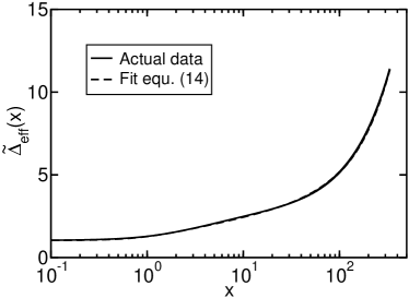
Figure 1: The dimensionless effective hybridization function $\tilde{\Delta}_{\rm eff}(x)$ evaluated for $\rho_{0}J=0.1$ in the SIKM. The resulting function is symmetric and is only plotted for $x>0$. It coincides with the universal form for $x\lesssim 30$. The dashed line represents the fit (14) and is nearly indistinguishable from the actual data. Notice especially the appearance of logarithmic behavior in the crossover region.

The following function provides an excellent fit (see Fig. 1)

$$\tilde{\Delta}_{\rm eff}(x)=\begin{array}[t]{l}\displaystyle 1+\frac{1}{2}\,a_{1}\ln\left(1+\left(\frac{x}{a_{0}}\right)^{2}\right)\\[14.22636pt] \displaystyle+a_{2}\left(\arctan\left|\frac{x}{a_{0}}\right|-\left|\frac{x}{a_{0}}\right|\right)\left(1-\ln\left|\frac{x}{a_{0}}\right|\right)\end{array}$$ (14)

with the parameters from Table 1.

$a_{0}$	$a_{1}$	$a_{2}$
0.829	0.536	0.00324

Table 1: Result of the fit (14) to the effective hybridization $\tilde{\Delta}_{\rm eff}(x)$.

A similar analysis based on the comparison of flow equations shows that the above mapping between the SIKM and the noninteracting RLM can be extended to the case of a Kondo Hamiltonian (1) with a nonvanishing local magnetic field $h$

$$H_{\rm SIKM}+g\mu_{B}\,h\,S_{z}$$ (15)

by setting $\epsilon_{d}=g\mu_{B}h$ in the RLM. However, the mapping with the above effective hybridization function becomes less accurate for $g\mu_{B}|h|\gtrsim T_{\rm K}$ due to the approximate nature of the flow equation solution (5–7). We will discuss this point in more detail below.

Summing up, as long as we are interested in static quantities in a local magnetic field smaller than approximately $T_{\rm K}$ and/or dynamical correlation functions for energies smaller than approximately $60T_{\rm K}$, we can use the RLM with the effective hybridization function (14) to describe the physics of the SIKM in the small coupling limit. The only undetermined parameter in the RLM is the energy scale $\Delta^{0}_{\rm eff}$ that explicitly depends on $J$. This overall energy scale is proportional to $T_{\rm K}$. Notice that the non–perturbative behavior of this energy scale

$$T_{\rm K}\propto e^{-1/\rho_{0}J}$$ (16)

follows correctly from the original flow equations (5–7), compare Ref. Hofstetter_Kehrein, .

II.3 Calculation of physical quantities

Once the mapping between the SIKM (1) and the effective RLM (8) has been established, one can readily calculate physical quantities for the Kondo model. One complication arises from the fact that operators of the original SIKM have to be transformed by a unitary transformation analogous to (2). In the language of the effective resonant level model they will thus in general correspond to more complicated many–particle operators. Since the intention of this paper is to demonstrate the potential of our mapping in a pedagogical setting, we will concentrate on two quantities that remain simple under these transformations: i) the $z$-component of the spin operator $S_{z}$, which becomes $S_{z}=d^{\dagger}d-1/2$, and ii) the Hamiltonian itself.

From the latter we obtain the internal energy $U_{\rm imp}=\langle H-H_{0}\rangle$ and the Sommerfeld coefficient, $\gamma_{\rm imp}(h)$. A straightforward calculation in the noninteracting RLM yields

$$\gamma_{\rm imp}(h)=\frac{\pi^{2}k_{\rm B}^{2}}{3}\rho_{d}(0)\left(1-\Lambda^{\prime}(0)\right)$$ (17)

where $\Lambda^{\prime}(\omega)$ denotes the derivative of

$$\Lambda(\omega)=\frac{1}{\pi}{\rm P}\int d\epsilon\>\frac{\Delta_{\rm eff}(\epsilon)}{\omega-\epsilon}$$

and ${\rm P}\int\ldots$ is the principal value integral. Here $\rho_{d}(\epsilon)$ is the impurity orbital density of states of the RLM

$$\rho_{d}(\epsilon)=\frac{1}{\pi}\,\frac{\Delta_{\rm eff}(\epsilon)}{(\epsilon-g\mu_{B}h-\Lambda(\epsilon))^{2}+\Delta_{\rm eff}^{2}(\epsilon)}\ .$$ (18)

The result (17) for $\gamma_{\rm imp}$ has some interesting implications. First, because $d^{\dagger}$ is connected to $S_{+}$, it is apparent that the low–energy excitations in the system are controlled by spin degrees of freedom, a well–known feature of the Kondo physics. However, in our approach this result can be read off directly from equ. (17). Second, $\rho_{d}(0)\propto 1/\Delta_{\rm eff}(0)\propto 1/T_{\rm K}$, i.e. we obtain the correct scaling behavior for $\gamma_{\rm imp}$ directly from the behavior of $\Delta_{\rm eff}(\epsilon)$. There is, however, a nontrivial correction coming from the factor in parenthesis in (17). Note that for $\Delta_{\rm eff}(\epsilon)=$const. this correction is one, but for the strongly $\epsilon$–dependent $\Delta_{\rm eff}(\epsilon)$ in Fig. 1 it is of the order of two. As we will demonstrate later, this difference is directly responsible for obtaining the correct Wilson ratio in our approach.

From the mapping $S_{z}=d^{\dagger}d-1/2$ it is easy to calculate $\chi_{zz}(\omega+i\delta)=-(g\mu_{B})^{2}\langle\langle d^{\dagger}d;d^{\dagger}d\rangle\rangle_{\omega+i\delta}$. Since the correlation function has to be evaluated within the RLM, one obtains for the imaginary part at $T=0$

$$\chi_{zz}^{\prime\prime}(\omega)=(g\mu_{B})^{2}\>\pi\int\limits_{-\omega}^{0}d\omega^{\prime}\>\rho_{d}(\omega^{\prime})\rho_{d}(\omega+\omega^{\prime})\ .$$ (19)

Again, this result provides direct access to an interpretation of the behavior of $\chi_{zz}(\omega+i\delta)$ in terms of the physics of the resonant level model.

III Results

One quantity that can be calculated analytically is the low–energy limit of the spin structure factor $S(\omega)\stackrel{{\scriptstyle\rm def}}{{=}}\chi^{\prime\prime}_{zz}(\omega)/\omega$,

$$S(0)=\lim_{\omega\rightarrow 0}\frac{\chi^{\prime\prime}_{zz}(\omega)}{\omega}\ .$$ (20)

For a vanishing local magnetic field $S(0)$ is just the spin relaxation rate accessible in e.g. spin resonance experiments. With the result for $\chi_{zz}^{\prime\prime}(\omega)$ from (19) we obtain

$$S(0)=(g\mu_{B})^{2}\>\frac{1}{\pi}\,\frac{\Delta_{\rm eff}^{2}(0)}{\left((g\mu_{B}h)^{2}+\Delta_{\rm eff}^{2}(0)\right)^{2}}\;\;,$$ (21)

which leads to the curve shown in Fig. 2. Eq. (21) is of particular importance because it explicitly demonstrates universality, $T_{\rm K}^{2}S(\omega)=f(g\mu_{B}h/T_{\rm K})$, and allows to directly fit e.g. experimental data from ESR or NMR experiments and extract the Kondo

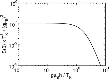
Figure 2: Universal curve for $S(0)$ as function of the local magnetic field $h$.

temperature. Note furthermore that the result (21) is not only valid in the Kondo limit, but also holds at the Toulouse point of the anisotropic Kondo model and everywhere in between. Since it does not depend on the details of $\Delta_{\rm eff}(\epsilon)$ it will also be true for general band structures $\epsilon_{\vec{k}}$ in (1) and thus is eventually the result for $S(0)$ in DMFT calculations.

The full frequency dependent $\chi_{zz}^{\prime\prime}(\omega)$ has to be calculated numerically using the form of the effective hybridization function in Fig. 1. The results for three values of the external field, $h=0$, $g\mu_{B}h=T_{\rm K}$ and $g\mu_{B}h=5T_{\rm K}$

Figure 3: $\chi_{zz}^{\prime\prime}(\omega)$ for three characteristic local magnetic fields $h=0$, $g\mu_{B}h=T_{\rm K}$ and $g\mu_{B}h=5T_{\rm K}$.

are displayed in Fig. 3. These correlation functions provide a good example for the usefulness of our mapping to the effective RLM since one can directly interpret the structures and their frequency and field dependencies in terms of analytical formulas derived for the RLM. E.g. the high–frequency behavior of $\chi_{zz}^{\prime\prime}(\omega)$ follows directly from equ. (19) and the behavior of the effective hybridization function $\Delta_{\rm eff}(\epsilon)$ at large energies (which is linear with logarithmic corrections, see Fig. 1): $\chi_{zz}^{\prime\prime}(\omega)$ decays like $1/\omega$ with logarithmic corrections, in agreement with (expensive) numerical results Costi99 .

For the dependence of the dynamical susceptibility on the local magnetic field one makes use of the fact that the local magnetic field corresponds to the on–site energy in the effective RML. Therefore it is obvious that the observed shift of the resonance peak in $\chi_{zz}^{\prime\prime}(\omega)$ is due to the shifted center of the resonant level. Furthermore, the depletion of the maximum value is related to the decreasing occupation of the resonant level, which corresponds directly to the increasing local magnetization in the SIKM. At the same time, one observes a decrease of the total spectral weight in $\chi_{zz}^{\prime\prime}(\omega)$, which can be accounted for by a transfer to a finite expectation value of $\langle S_{z}\rangle$ in the SIKM. There is, however, also a non–trivial effect, namely the increasing broadening of the resonance peak with increasing magnetic field. For a RLM with a constant $\Delta_{\rm eff}(\epsilon)$ such a behavior does not occur; it is entirely related to the fact that with increasing magnetic field the system starts to notice the energy dependence of the effective hybridization.

The quantity not yet fixed in our calculation is $T_{\rm K}$, or more precisely the proportionality constant in $T_{\rm K}\propto\Delta_{\rm eff}(0)$. This can most conveniently be done by using Wilson’s definition of the Kondo temperaturehewson

$$\chi_{0}(h=0)=(g\mu_{B})^{2}\,\frac{w}{4T_{\rm K}}\;\;,$$ (22)

where $\chi_{0}$ is the static magnetic susceptibility and $w=0.413$ the Wilson number. $\chi_{0}$ can be obtained from the imaginary part of the dynamic susceptibility (19) via

$$\chi_{0}=\frac{2}{\pi}\int\limits_{0}^{\infty}d\omega\,\frac{\chi^{\prime\prime}_{zz}(\omega)}{\omega}$$ (23)

and must in general be evaluated numerically. At the Toulouse point one can, however, give an analytic answer since $\Delta_{\rm eff}(\omega)={\rm const.}$ and thus

$$\chi_{0}(h)=(g\mu_{B})^{2}\>\frac{1}{\pi}\,\frac{\Delta_{\rm eff}(0)}{h^{2}+\Delta_{\rm eff}(0)^{2}}\;\;.$$ (24)

Therefore at the Toulouse point the Korringa–Shiba relationKorringaShiba

$$R_{\rm S}=\frac{(g\mu_{\rm B})^{2}}{2\pi\chi_{0}^{2}}\lim_{\omega\to 0}\frac{\chi_{zz}^{\prime\prime}(\omega)}{\omega}$$ (25)

is independent of the local magnetic field

$$R_{\rm S}=\frac{(g\mu_{B})^{2}\,S(0)}{2\pi\chi_{0}^{2}(h)}=\frac{1}{2}\ .$$ (26)

In the following we will discuss $\chi_{0}(h)$ and the Korringa–Shiba relation for the Kondo limit $\rho_{0}J\rightarrow 0$. The quantity $\chi_{0}(h)$ is particularly convenient for a comparison with NRG results.

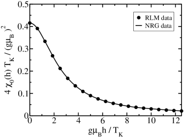
Figure 4: The magnetic susceptibility $\chi_{0}(h)$ from equ. (23) (circles) and the same quantity obtained from an NRG calculation.

In Fig. 4 the circles represent the values of $\chi_{0}(h)$ calculated via (23) with the effective hybridization function from Fig. 1, and the full line represents the result of an NRG calculation. We observe excellent agreement for all values of the local magnetic field: notice that the curves agree without fit parameters. This example clearly demonstrates that the nontrivial form of the effective hybridization in Fig. 1 encodes the many–particle physics of the SIKM in a trivial noninteracting effective model.

The result in Fig. 4 can readily be combined with relations (17) and (21) to obtain the Wilson ratioWilson

$$R_{\rm W}=\frac{4\pi^{2}k_{\rm B}^{2}}{3(g\mu_{\rm B})^{2}}\frac{\chi_{\rm imp}(h)}{\gamma_{\rm imp}(h)}\ .$$ (27)

Our results for the Wilson ratio and the Korringa–Shiba relation obtained within the effective RLM are collected in Fig. 5. For the Wilson ratio we would actually have to calculate the quantity $\chi_{\rm imp}$ and not $\chi_{0}$.Wilson However, for the case of small $\rho_{0}J$ considered here, both quantities are equivalent.chen One observes that both $R_{\rm W}$ and $R_{\rm S}$ are independent of the local magnetic field up to approximately $g\mu_{B}h\approx T_{\rm K}$, and then start to

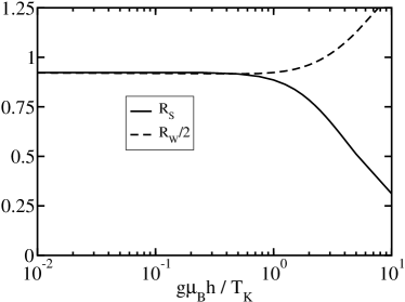
Figure 5: Results for the Shiba ratio $R_{\rm S}$ (full line) and the Wilson ratio $R_{\rm W}$ (dashed line) as a function of a local magnetic field. The correct limiting values at $h\to 0$ are missed by approximately 5%.

decrease (Shiba ratio), respectively increase (Wilson ratio). The exact Bethe ansatz solution bethe gives $R_{\rm W}(h)=2$ independent of the magnetic field strength (see also Ref. logan3, ), and local Fermi liquid theory yields $R_{\rm S}=1$ for $h\rightarrow 0$.hewson Our limiting values as $h\to 0$ miss these exact results by approximately 5%. Notice that the term $(1-\Lambda^{\prime}(0))$ in (17) is very important to obtain this correct value for $R_{\rm W}(h=0)$. Remarkably, our simple noninteracting effective model therefore correctly describes the Wilson ratio in the Kondo limit (for not too large magnetic fields), which is a hallmark of strong–coupling Kondo physics.

Let us finally analyze the accuracy of our effective model. Since Fig. 4 demonstrates that integral quantities like $\chi_{0}(h)$ are obtained with very good accuracy for all magnetic fields, one can infer from Fig. 5 that quantities depending on low–energy details in frequency space like $\gamma_{\rm imp}$ and $S(0)$ are more susceptible to our approximations for increasing magnetic fields. This suggests that for such low–energy quantities our effective model can be employed with very good accuracy (5% error) for magnetic fields below $T_{\rm K}$, and with good accuracy (20% error) still up to approximately $5T_{\rm K}$.

IV Summary and outlook

Summing up, we have shown that the resonant level model with a nontrivial hybridization function $\Delta_{\rm eff}(\epsilon)$ can be used as an effective model for the single impurity Kondo model. The key observation was the fact that the flow equation solutions of both models are approximately identical if a suitable $\Delta_{\rm eff}(\epsilon)$ is chosen for the RLM (Fig. 1). In this mapping the impurity orbital occupation number $n_{d}-1/2$ plays the role of the Kondo impurity spin $S_{z}$. The impurity orbital energy corresponds to the local magnetic field acting on $S_{z}$.

In contrast with the conventional approach where effective models describe the vicinity of the low–energy renormalization group fixed pointsWilson ; hewson , our effective model very accurately describes both certain low– and high–energy properties of the original Kondo model: compare for example our discussion of the dynamical spin–spin correlation function in Fig. 3. It also yields thermodynamic quantities that are in excellent agreement with much more expensive numerical methods (see Fig. 4). The nontrivial behavior of the effective hybridization function encodes the quasiparticle interaction, which leads to e.g. the correct Wilson ratio for small magnetic fields (with 5% accuracy). Notice, however, that our effective model does not allow the correct evaluation of higher–order correlation functions beyond the low–energy limit,

In conclusion, our approach describes many aspects of the complicated many–body Kondo physics for not too large magnetic fields within a simple noninteracting model. Therefore one can very easily and intuitively understand certain properties of the Kondo model, e.g. the dependence of correlation functions on a local magnetic field (Fig. 3). One main prospect of our approach is to look at other correlation functions using this effective model, in particular the $T$–matrix for applications in the framework of DMFT calculations. Future prospects also include cluster problems and the single impurity Anderson model. Work along these lines is in progress.

- (1) J. Kondo, Prog. Theor. Phys. 32, 27 (1964).
- (2) P. W. Anderson, Phys. Rev. 124, 41 (1961).
- (3) For a comprehensive overview see e.g. A. C. Hewson, The Kondo Problem to Heavy Fermions (Cambridge Univ. Press, 1993). Cambridge, 1993.
- (4) N. Andrei, K. Furuya, and J. H. Lowenstein, Rev. Mod. Phys. 55, 331 (1983); A. M. Tsvelick and P. B. Wiegmann, Adv. Phys. 32, 453 (1983).
- (5) K. G. Wilson, Rev. Mod. Phys. 47, 773 (1975); H. R. Krishna-murthy, J. W. Wilkins and K. G. Wilson, Phys. Rev. B 21, 1003 & 1044 (1980).
- (6) J.E. Hirsch and R.M. Fye, Phys. Rev. Lett. 56, 2521 (1986).
- (7) M. Jarrell and J.E. Gubernatis, Phys. Rep. 269, 135 (1996).
- (8) T. Costi, Phys. Rev. Lett. 85, 1504 (2000).
- (9) M. T. Glossop and D. E. Logan, J. Phys. – Condens. Matter 13, 9713 (2002).
- (10) D. E. Logan, M. P. Eastwood, and M. A. Tusch, J. Phys. – Condens. Matter 10, 2673 (1998); D. E. Logan and M. T. Glossop, J. Phys. – Condens. Matter 12, 985 (2000).
- (11) R. Bulla, M. T. Glossop, D. E. Logan, and Th. Pruschke, J. Phys. – Condens. Matter 12, 4899 (1998).
- (12) D. E. Logan and N. L. Dickens, Europhys. Lett. 54, 227 (2001).
- (13) W. Metzner and D. Vollhardt, Phys. Rev. Lett. 62, 324 (1989); A. Georges, G. Kotliar, W. Krauth and M.J. Rozenberg, Rev. Mod. Phys. 68, 13 (1996).
- (14) F. Wegner, Ann. Physik (Leipzig) 3, 77 (1994).
- (15) S. Kehrein, Phys. Rev. Lett. 83, 4914 (1999); S. Kehrein, Nucl. Phys. B[FS] 592, 512 (2001).
- (16) W. Hofstetter and S. Kehrein, Phys. Rev. B 63, 140402(R) (2001).
- (17) For an overview of bosonization and refermionization techniques see e.g. J. von Delft and H. Schoeller, Ann. Physik (Leipzig) 7, 225 (1998).
- (18) The investigation of nontrivial dispersion relations is one of the main future perspectives of the flow equation approach. Work along these lines is in progress.
- (19) S. Kehrein, to be published.
- (20) S. Kehrein and A. Mielke, Ann. Phys. (New York) 252, 1 (1996).
- (21) G. Toulouse, C. R. Acad. Sci. Paris 268, 1200 (1969).
- (22) It becomes increasingly difficult to numerically investigate smaller couplings.
- (23) T.A. Costi and C. Kieffer, Phys. Rev. Lett. 76, 1683 (1996).
- (24) H. Shiba, Prog. Theor. Phys. 54, 967 (1975).
- (25) K. Chen, C. Jayaprakash, and H. R. Krishnamurthy, Phys. Rev. B 45, 5368 (1992).