Reliability Polynomials and their Asymptotic Limits for Families of Graphs

Shu-Chiuan Chang and Robert Shrock
C. N. Yang Institute for Theoretical Physics

State University of New York

Stony Brook, NY 11794-3840

We present exact calculations of reliability polynomials $R(G,p)$ for lattice strips $G$ of fixed widths $L_{y}\leq 4$ and arbitrarily great length $L_{x}$ with various boundary conditions. We introduce the notion of a reliability per vertex, $r(\{G\},p)=\lim_{|V|\to\infty}R(G,p)^{1/|V|}$ where $|V|$ denotes the number of vertices in $G$ and $\{G\}$ denotes the formal limit $\lim_{|V|\to\infty}G$. We calculate this exactly for various families of graphs. We also study the zeros of $R(G,p)$ in the complex $p$ plane and determine exactly the asymptotic accumulation set of these zeros ${\cal B}$, across which $r(\{G\})$ is nonanalytic.

keywords: reliability polynomial, Potts model, Tutte polynomial

1 Introduction

With the development of progressively larger communications networks such as those involving telecommunications and those connecting computers, from large local area networks to the internet, the analysis of the reliability of these networks has become an increasingly important area of study. Because many types of failures of communication links are random, this study falls within the area of statistical physics, as well as engineering and, as will be evident, mathematical graph theory. A common approach to this study is to factorize the reliability into a factor describing the components such as message routers and computers at various nodes, on the one hand, and the links between these nodes, on the other hand. One often assumes that nodal network elements like message routers and computers have a certain probability $p_{node}$ of (normal) operation. Since failures of these nodal components generally occur independently, the factor in the overall reliability due to these elements is then $p_{node}^{n}$, where $n$ is the number of nodes in the network. The other factor contributing to the overall network reliability involves the connecting links on the network and hence the connectivity structure of the network. As mentioned above, many failures in these connecting links are also random and independent and may thus be treated in a probabilistic manner in which one describes a given link as having a probability $p$ of operating and thus a probability $1-p$ of failing. (Examples of nonrandom failures include earthquakes that affect only one portion of a network; these are not considered here.) The network is thus represented as a connected graph $G=(V,E)$ with vertex (= node) set $V$ and edge (= bond) set $E$, in which each vertex represents either a message router or switch or an endpoint such as a computer or terminal (or telephone in the telecommunications example) and each edge represents the link between the nodes. We shall be interested here in a commonly used simplified model of the network in which each nodal element and link have, respectively, the same fixed probabilities $p_{node}$ and $p$ of operation with $p_{node}$ and $p$ lying in the interval $[0,1]$. We shall denote the number of vertices and edges in $G$ as $|V|=n$ and $|E|$. In the graphical representation of the network, one regards a normally operating communications link as an edge that is present (with probability $p$), and a malfunctioning communications link as an edge that is absent (with probability $1-p$), the presence or absence being random and uncorrelated. Defining a successfully operating network as one in which all of links and nodes are operating normally, it follows that the node reliability is, as noted above, $p_{node}^{|V|}$, independent of the connectivity of the network. The factor due to the operation of the links is much more difficult to calculate. It is therefore customary, in modelling the reliability behavior of networks, to separate out the node-reliability factor and concentrate on the contribution due to the structure of the network.

The all-terminal reliability polynomial $R(G,p)$ is defined as the probability that there is an operating communications link between any two nodes in the network, i.e. any two vertices in the set $V$ are connected (by a path consisting of edges that are present) [2]-[6]. In passing, we note that one can also study $k$-terminal reliability probability polynomials, but we shall restrict ourselves here to the all-terminal reliability polynomial and hence shall henceforth omit the qualifier “all-terminal” in the notation. The contributions to $R(G,p)$ arise from the sum of connected spanning subgraphs of $G$. Here a spanning subgraph is a subgraph $G^{\prime}=(V,E^{\prime})$ with $E^{\prime}\subseteq E$, i.e. a graph with the same vertex set and a subset of the edge set of $G$. Denote a connected spanning subgraph as $H=(V,E_{H})$. Each contribution to $R(G,p)$ is weighted by a factor $p^{|E_{H}|}$ reflecting the probability that the $|E_{H}|$ edges are present, multiplied by a factor $(1-p)^{|E|-|E_{H}|}$ reflecting the probability that the edges in the complement set $\{e\in E;e\not\in E_{H}\}$, of cardinality $|E|-|E_{H}|$, are absent. That is,

$$R(G,p)=\sum_{H\subseteq G}p^{|E_{H}|}(1-p)^{|E|-|E_{H}|}\ .$$ (1.1)

Some pioneering studies of network reliability include [2]-[5]; a review is [6]. The calculation of $R(G,p)$ for an arbitrary (connected) graph $G$ has been proved to be #-P complete [6, 7]; that is, roughly speaking, for a generic network $G$, the time required to calculate $R(G,p)$ grows exponentially with the size of the network. In the face of this difficulty, network designers have often relied upon upper and lower bounds on $R(G,p)$ [8]- [14]. It is clearly of interest if one can obtain exact solutions for $R(G,p)$ for some families of graphs $G$.

In this paper, we shall present a number of such exact solutions for reliability polynomials, for recursive families of graphs $G$. We have previously presented such solutions for a specific recursive family of graphs in [15]. A recursive family of graphs is one in which one constructs successive members of the family in a recursive manner starting from an initial member. Recursive families of graphs that are of particular interest here are strips of regular lattices of a given width $L_{y}$ vertices and arbitrarily great length $L_{x}$ vertices with some specified transverse and longitudinal boundary conditions. We shall envision these strips as extending in the horizontal (= longitudinal, $x$) direction and having transverse extent in the vertical, $y$, direction. To see that these form recursive families, one can picture a strip, say of the square lattice, of length $L_{x}$ and width $L_{y}$ as being formed by gluing on a column of squares of height $L_{y}$ to the strip of length $L_{x}-1$. The boundary conditions that we shall consider include free (FBC), periodic (PBC), and twisted periodic (TPBC), by which is meant that the longitudinal ends are identified with a reversal of orientation. We shall denote the various combinations as (i) $(FBC_{y},FBC_{x})=$ free, (ii) $(FBC_{y},PBC_{x})=$ cyclic, (iii) $(FBC_{y},TPBC_{x})=$ Möbius, (iv) $(PBC_{y},FBC_{x})=$ cylindrical, (v) $(PBC_{y},PBC_{x})=$ torus, and (vi) $(PBC_{y},TPBC_{x})=$ Klein bottle. For an arbitrary graph $G$, one defines the degree $d_{i}$ of a vertex $v_{i}$ as the number of edges connected to it. One then defines the maximum degree as $\Delta=\max_{v_{i}\in V}d_{i}$. A $\Delta$-regular graph is one in which all of the vertices have the same degree $\Delta$. Some strip graphs, such as those with toroidal or Klein bottle boundary conditions, are $\Delta$-regular graphs. For strip graphs that are not $\Delta$-regular, it will still be useful to define an average or effective vertex degree in the limit of infinite length, namely

$$d_{eff}=\lim_{|V|\to\infty}\frac{2|E|}{|V|}\ .$$ (1.2)

Secondly, we shall introduce a definition of the reliability per node in the limit of many nodes,

$$r(\{G\},p)=\lim_{|V|\to\infty}R(G,p)^{1/|V|}$$ (1.3)

where $\{G\}$ denotes the formal limit of a given family, $\lim_{|V|\to\infty}G$. We calculate this function exactly for a number of families and study its properties. As we shall show, this function provides a convenient quantitative measure of the reliability properties of large networks.

A third part of our work involves the calculation of the zeros of $R(G,p)$ in the complex $p$ plane and the determination of their asymptotic continuous accumulation set, denoted ${\cal B}$ as the number of vertices $|V|\to\infty$ (in practice, for our strips, this is equivalent to the limit of infinite length, $L_{x}\to\infty$). As we shall show, the function $r(\{G\})$ is nonanalytic across the locus ${\cal B}$. We define $p_{c}$ as the maximal point where ${\cal B}$ intersects (or coincides with) the real axis. For the infinite-length limits of some lattice strips, the locus ${\cal B}$ does not cross the real axis, so no $p_{c}$ is defined. In certain of these cases, there are complex-conjugate arcs on ${\cal B}$ whose endpoints at $p_{end},p_{end}^{*}$ are very close to the real axis; in these cases, it is useful to define a $(p_{c})_{eff}=Re(p_{end})$. Although the width $L_{y}\to\infty$ limit of loci ${\cal B}$ for the infinite-length lattice strips is not necessarily the same as the continuous accumulation locus of the zeros of the reliability polynomial for the two-dimensional thermodynamic limit $L_{x}\to\infty$, $L_{y}\to\infty$ with $L_{y}/L_{x}$ fixed to a finite nonzero constant, our exact results on infinite-length limits of lattice strip graphs can give some insight into plausible behavior of the locus ${\cal B}$ for the thermodynamic limits of the corresponding 2D lattices. We shall discuss this further below.

There are several motivations for our study. Clearly, new exact calculations of reliability polynomials are of interest from the point of view of both the statistical physics of network theory and of mathematical graph theory. The generalization of $p$ from the interval $p\in[0,1]$ to $p\in{\mathbb{C}}$ is clearly necessary in order to analyze the zeros of the reliability polynomial and their accumulation set as $|V|\to\infty$. Our results also further illuminate the fascinating variety of applications of the Tutte polynomial, or equivalently, the Potts model partition function. Our focus here is thus somewhat more abstract than in a specific engineering context, where one is trying to design the most reliable network subject to various constraints, such as cost.

2 Some General Properties of the Reliability Polynomial

In this section we review some general properties of the reliability polynomial that will be used in the rest of the paper. As is evident from its definition, the reliability polynomial has the properties that

$$R(G,0)=0\ ,\quad R(G,1)=1,$$ (2.1)

$${\rm If}\ \ p\in[0,1],\quad{\rm then}\quad R(G,p)\in[0,1]$$ (2.2)

and

$$\frac{dR(G,p)}{dp}\geq 0\quad{\rm for}\quad p\in[0,1]\ .$$ (2.3)

In general, an edge can be classified as (i) a loop, i.e., an edge that connects a vertex to itself, (ii) a bridge (= co-loop) with the property that if it is deleted, this increases the number of connected components of the graph by one (so that, if $G$ is connected, deleting the bridge breaks $G$ into two disjoint parts), or (iii) neither a loop nor a bridge. We shall use the standard mathematical notation that $G/e$ means the graph obtained by deleting $e$ and identifying the two vertices that were connected by $e$ (called contracting $G$ on $e$) and $G-e$ means the graph obtained by deleting $e$. Now if $e$ is a loop, $e=e_{\ell}$, then the probability that all terminals are connected with each other is independent of $e_{\ell}$, so

$$R(G,p)=R(G/e_{\ell},p)\ .$$ (2.4)

If $e=e_{b}$ is a bridge, then the probability that it is present is an overall multiplicative factor in $R$, so

$$R(G,p)=pR(G/e_{b},p)\ .$$ (2.5)

If $e$ is neither a loop nor a bridge, then $R(G,p)$ satisfies the deletion-contraction relation

$$R(G,p)=(1-p)R(G-e,p)+pR(G/e,p)\ .$$ (2.6)

That is, if the edge $e$ is not present, then $R(G,p)$ has the value given by the reliability polynomial of a graph $G-e$ times the factor $(1-p)$; if the edge is present, then $R(G,p)$ has the same value as the reliability polynomial of a graph contracted on $e$, multiplied by $p$, and since these two possibilities ($e$ not present or present) are mutually exclusive and exhaust the possibilities, the full polynomial $R(G,p)$ is the sum of these two possibilities.

We next comment on some general properties of our $r(\{G\},p)$ function. We recall that a tree graph $T_{n}$ is a connected graph with $n$ vertices and no circuits. Since $R(T_{n},p)=p^{n-1}$, it follows that $r(\{T\},p)=p$, where $\{T\}\equiv\lim_{n\to\infty}T_{n}$. However, in general, $r$ differs from $p$ for network topologies that are more complicated than that of a tree graph. The $r$ function can give insight into the reliability behavior of large networks. From obvious arguments, it follows that any reliability function, whether the $k$-terminal reliability function $R_{k}(G,p)$ or the all-terminal reliability $R_{A}(G,p)$, is a monotonically increasing function of $p$ on the relevant interval $p\in[0,1]$. It follows that $r(\{G\},p)$ is also a monotonically nondecreasing function of $p$ on this interval.

From the basic definition (1.1) one can generalize $p$ from the physical interval $0\leq p\leq 1$ to arbitrary real or, indeed, complex $p$. This generalization is necessary when one calculates the zeros of $R(G,p)$ in the complex $p$ plane. Using our calculations of $R(G,p)$ for a variety of families of lattice strip graphs, we shall determine exactly the continuous accumulation set of the zeros of $R(G,p)$ in the complex $p$ plane as $|V|\to\infty$ for each family of graphs $G$. We shall denote this accumulation set as ${\cal B}$. In this context we note that in 1992 Brown and Colbourn conjectured that for an arbitrary connected graph $G$, all of the zeros of the reliability polynomial $R(G,p)$ lie in the disk $|p-1|\leq 1$ [16] (some related work is [17, 18, 19]). Recently, Royle and Sokal have reported counterexamples that show the Brown-Colbourn conjecture to be false [20], although the maximal values of $|p-1|$ found so far are only slightly greater than unity. Extending the counterexamples found in [20], we have also found several recursive families of graphs for which the conjecture is false.

One can also address a related question for the continuous asymptotic accumulation set ${\cal B}$: Consider a recursive family of arbitrary connected graphs $G=G(V,E)$ and, as above, let ${\cal B}$ be the asymptotic accumulation set of zeros of $R(G,p)$ in the limit $|V|\to\infty$. Is it true that all points on ${\cal B}$ are contained in the disk disk $|p-1|\leq 1$? Clearly, although the Brown-Colbourn conjecture is false, the answer to the above question could still be yes since the zeros of $R(G,p)$ that lie outside the disk $|p-1|$ might, a priori, not accumulate to form part of ${\cal B}$. However, we shall show that the answer to this question is no, i.e. we shall exhibit recursive families of graphs for which ${\cal B}$ extends outside the disk $|p-1|$. Using our exact results, we shall address a number of other interesting questions concerning ${\cal B}$. It is also of interest to note that Brown and Colbourn proved that all of the real roots of the reliability polynomial lie in the set $\{0\}\cup(1,2]$ [16].

Since we shall present calculations for strip graphs with free and periodic or twisted periodic longitudinal boundary conditions, we observe the following inequality, where $BC_{y}$ refers to any given transverse boundary condition

Theorem 2.1

For a strip graph $G_{s}$ of length $L_{x}$ and width $L_{y}$ vertices,

$$R(G_{s},L_{y}\times L_{x},BC_{y},(T)PBCx,p)\geq R(G_{s},L_{y}\times L_{x},BC_{y},FBC_{x},p)$$ (2.7)

Proof  These inequalities follow because for a given type of lattice strip graph $G_{s}$ with a given length $L_{x}$ and width $L_{y}$, the strip with periodic or twisted periodic longitudinal boundary conditions has a greater connectivity than strip with free longitudinal boundary conditions. In particular, for a given $G_{s}$, if all of the transverse edges at a fixed longitudinal location are absent, this does not produce two disjoint graphs for a cyclic or Möbius strip but does for the free strip. $\Box$.

3 Relations Between the Reliability Polynomial and the Tutte Polynomial and Potts Model Partition Function

We recall that the Tutte polynomial of a graph $G=(V,E)$ is [21]-[28]

$$T(G,x,y)=\sum_{G^{\prime}\subseteq G}(x-1)^{k(G^{\prime})-k(G)}(y-1)^{c(G^{\prime})}$$ (3.1)

where $k(G^{\prime})$ and $c(G^{\prime})$ denote the number of components and linearly independent circuits of $G^{\prime}$, with $c(G^{\prime})=|E^{\prime}|+k(G^{\prime})-|V|$. Since we deal only with connected graphs here, $k(G)=1$. (We follow standard notation for the variables $x$ and $y$ of the Tutte polynomial and caution the reader that these have no connection with the $x$ (longitudinal) and $y$ (transverse) axes of the strip graphs.) The reliability polynomial $R(G,p)$ can be expressed in terms of the Tutte polynomial $T(G,x,y)$ as [6]

$$R(G,p)=p^{|V|-1}(1-p)^{|E|-|V|+1}T(G,1,\frac{1}{1-p})\ .$$ (3.2)

We shall use this relation to calculate reliability polynomials for various families of graphs from our previous calculations of the Tutte polynomials for these graphs [29]-[39]. We have also used an iterative application of the deletion-contraction relation (2.6) to calculate reliability polynomials directly.

The Tutte polynomial is equivalent to the partition function of the Potts spin model. On a lattice, or more generally, on a graph $G$, at temperature $T$, this model is defined by the partition function [40, 41]

$$Z(G,q,v)=\sum_{\{\sigma_{i}\}}e^{-\beta{\cal H}}$$ (3.3)

with the Hamiltonian

$${\cal H}=-J\sum_{\langle ij\rangle}\delta_{\sigma_{i}\sigma_{j}}$$ (3.4)

where $\sigma_{i}=1,...,q$ are the spin variables on each vertex $i\in G$; $\beta=(k_{B}T)^{-1}$; $\langle ij\rangle$ denotes pairs of adjacent vertices; and we use the notation

$$K=\beta J\ ,\quad a=e^{K}\ ,\quad v=a-1\ .$$ (3.5)

This partition function can be written as [42]

$$Z(G,q,v)=\sum_{G^{\prime}\subseteq G}q^{k(G^{\prime})}v^{e(G^{\prime})}\ .$$ (3.6)

This formula enables one to generalize $q$ from ${\mathbb{Z}}_{+}$ to ${\mathbb{R}}$ or, indeed, ${\mathbb{C}}$. From it one also directly deduces the equivalence

$$Z(G,q,v)=(x-1)^{k(G)}(y-1)^{|V|}T(G,x,y)$$ (3.7)

where

$$x=1+\frac{q}{v}$$ (3.8)

and

$$y=v+1=e^{K}$$ (3.9)

so that

$$q=(x-1)(y-1)\ .$$ (3.10)

Combining (3.2) and (3.7), we have, for a connected graph $G$, the relation between the reliability polynomial and the Potts model partition function

$$R(G,p)=(1-p)^{|E|}\ \lim_{q\to 0}\ q^{-1}Z(G,q,v=\frac{p}{1-p})\ .$$ (3.11)

Note that $Z(G,q,v)$ always has an overall factor of $q$, which cancels the factor of $q^{-1}$ in (3.11). The valuation $y=1/(1-p)$ in (3.2), or equivalently, $v=p/(1-p)$ in (3.11) can also be expressed as

$$p=1-e^{-K}=\frac{v}{1+v}\ .$$ (3.12)

Thus the physical range of $p\in[0,1]$ for the network corresponds to the physical range of temperature for the $q=0$ Potts ferromagnet, with $T=0\ \Leftrightarrow\ p=1$ and $T=\infty\ \Leftrightarrow\ p=0$. The physical range of temperature for the Potts antiferromagnet would correspond to the unphysical interval $-\infty\leq p\leq 0$ for the network.

4 Structural Results

4.1 General Recursive Families of Graphs

A general form for the Tutte polynomial for the strip graphs considered here, or more generally, for recursively defined families of graphs $G_{m}$ comprised of $m$ repeated subgraph units, is [29]

$$T(G_{m},q,v)=\frac{1}{x-1}\sum_{j=1}^{N_{T,G,\lambda}}c_{G,j}(\lambda_{G,j})^{m}$$ (4.1.1)

where the terms $\lambda_{G,j}$, the coefficients $c_{G,j}$, and the total number $N_{Z,G,\lambda}$ depend on $G$ through the type of lattice, its width, $L_{y}$, and the boundary conditions, but not on the length.

We observe the following general result:

Theorem 4.1

Consider a recursive family of graphs $G_{m}$ comprised of $m$ repeated subgraph units. Then the reliability polynomial $R(G_{m},p)$ has the general form

$$R(G_{m},p)=\sum_{j=1}^{N_{R,G,\mu}}c_{R,G,j}(\mu_{G,j})^{m}$$ (4.1.2)

where the coefficients $c_{R,G,j}$ and terms $\mu_{G,j}$’s depend on $G$ through the type of lattice, its width, $L_{y}$, and the boundary conditions, but not on the length.

Proof  This is proved by combining (3.2) and (4.1.1). Clearly, the $\mu_{G,j}$’s and $c_{R,G,j}$’s can be determined from the $\lambda_{G,j}$’s and $c_{G,j}$’s. $\Box$ The reduction of the form (4.1.1) to (4.1.2) is analogous to the reduction that we had found for chromatic polynomials of recursive families of graphs [43]-[51].

It is convenient to factor out a power of $p$ and write (4.1.2) as

$$R(G_{m},p)=p^{a_{1,G}m+a_{0,G}}\sum_{j=1}^{N_{R,G,\alpha}}c_{R,G,j}(\alpha_{G,j})^{m}$$ (4.1.3)

with

$$\alpha_{G,j}=p^{-a_{1,G}}\mu_{G,j}$$ (4.1.4)

where again the $a_{i,G}$, $i=0,1$, depend on $G$ through the type of lattice, its width, $L_{y}$, and the boundary conditions, but not on the length. Obviously, $N_{R,G,\alpha}=N_{R,G,\mu}$. We find that for $p=1$, for all of the families that we have considered, all except one of the $N_{R,G,\alpha}$ $\alpha_{G,j}$’s vanish, and the nonzero term, which can be taken to be the first, has the value unity:

$$\alpha_{G,1}=1\ ,\quad\alpha_{G,j}=0\ ,\quad 2\leq j\leq N_{R,G,\alpha}\quad{\rm for}\ \ p=1$$ (4.1.5)

For the strips of the square and triangular lattices considered here,

$$a_{1,G}=L_{y}\ ,\quad G\ \ {\rm of}\ \ sq,t\ \ {\rm type}$$ (4.1.6)

and for the strips of the honeycomb lattice,

$$a_{1,G}=2L_{y}\ ,\quad G\ \ {\rm of}\ \ hc\ \ {\rm type}$$ (4.1.7)

Note that for all of the strips of the square and triangular lattice with periodic or twisted periodic longitudinal boundary conditions, $m=L_{x}$. For the corresponding strips with free longitudinal boundary conditions, it is convenient to set $m=L_{x}-1$; with this definition, it follows that for strips with both free and periodic (or twisted periodic) longitudinal boundary conditions, $m$ is equal to length measured in units of edges, with $L_{x}$ being the length in terms of vertices. The situation with the honeycomb strips is different. For example, for a cyclic strip of the honeycomb lattice, envisioned as a brick lattice, $L_{x}=2m$; that is, if the strip is $m$ bricks long, then the length, measured in terms of vertices, is $2m$.

Following our earlier nomenclature [43], we denote a term $\alpha_{G,j}$ in (4.1.3) as leading (= dominant) if it has a magnitude greater than or equal to the magnitude of other $\alpha_{G,j^{\prime}}$’s. In the limit $n\to\infty$ the leading $\alpha_{G,j}$ in $R(G,p)$ determines the function $r(\{G\},p)$. The continuous locus ${\cal B}$ where $r(\{G\},p)$ is nonanalytic thus occurs where there is a switching of dominant $\alpha_{G,j}$’s in $R$, respectively, and is the solution of the equation of degeneracy in magnitude

$$|\alpha_{G,j}|=|\alpha_{G,j^{\prime}}|$$ (4.1.8)

between two dominant $\alpha$’s.

4.2 Cyclic Strips of Regular Lattices

Here we will derive some structural properties of reliability polynomials for cyclic strips of regular lattices from corresponding properties of Tutte polynomials, using eq. (3.2). In [32] it was shown that for cyclic and Möbius strips of the square lattice of fixed width $L_{y}$ and arbitrary length $L_{x}$ (and also for cyclic strips of the triangular lattice) the coefficients $c_{j}$ in the Tutte polynomial are polynomials in $q$ with the property that for each degree $d$ there is a unique polynomial, denoted $c^{(d)}$. Further, this was shown to be

$$c^{(d)}=U_{2d}(q^{1/2}/2)=\sum_{j=0}^{d}(-1)^{j}{2d-j\choose j}q^{d-j}$$ (4.2.1)

where $U_{n}(x)$ is the Chebyshev polynomial of the second kind. A number of properties of these coefficients were derived in [32]. The first few of these coefficients are

$$c^{(0)}=1\ ,\quad c^{(1)}=q-1\ ,\quad c^{(2)}=q^{2}-3q+1\ ,$$ (4.2.2)

$$c^{(3)}=q^{3}-5q^{2}+6q-1\ .$$ (4.2.3)

Following our earlier work [37], we define

$$\kappa^{(d)} = c^{(d)}+c^{(d-1)}$$ (4.2.4)

$$= \sum_{j=0}^{d-1}(-1)^{j}{2d-1-j\choose j}q^{d-j}$$ (4.2.6)

and

$$\bar{\kappa}^{(d)}=q^{-1}\kappa^{(d)}=\sum_{j=0}^{d-1}(-1)^{j}{2d-1-j\choose j}q^{d-1-j}\ .$$ (4.2.7)

An important property of $\kappa^{(d)}$ is that it always has the factor $q$; this is evident from (4.2.6). The first few of these polynomials are

$$\kappa^{(1)}=q\ ,\quad\kappa^{(2)}=q(q-2)\ ,\quad\kappa^{(3)}=q(q-1)(q-3)\ .$$ (4.2.8)

The following special results for $q=0$, i.e., $x=1$, will be useful:

$$\lim_{q\to 0}\bar{\kappa}^{(d)}=(-1)^{d+1}d$$ (4.2.9)

$$c^{(d)}=(-1)^{d}\quad{\rm for}\quad q=0$$ (4.2.10)

and

$$\frac{dc^{(d)}}{dq}=(-1)^{d-1}\frac{(d+1)d}{2}\quad{\rm for}\ \ q=0$$ (4.2.11)

so that, using (3.10) to express $c^{(d)}$ as a function of $x$ and $y$,

$$\frac{\partial c^{(d)}}{\partial x}=(-1)^{d-1}(y-1)\frac{(d+1)d}{2}\quad{\rm for}\ \ x=1\ .$$ (4.2.12)

The terms $\lambda_{T,G_{s},L_{y},j}$ that occur in (4.1.1) can be classified into sets, with the $\lambda_{T,G_{s},L_{y},j}(x,y)$ in the $d$’th set being defined as those terms with coefficient $c^{(d)}$. In Ref. [32] the numbers of such terms, denoted $n_{T}(L_{y},d)$, were calculated. Labelling the eigenvalues with coefficient $c^{(d)}$ as $\lambda_{T,G_{s},L_{y},d,j}$ with $1\leq j\leq n_{T}(L_{y},d)$, the Tutte polynomial for a strip graph of length $L_{x}=m$ of a regular lattice of type $G_{s}$ can be written in the form

$$T[G_{s}(L_{y}\times m;FBC_{y},PBC_{y}),x,y]=\frac{1}{x-1}\sum_{d=0}^{L_{y}}c^{(d)}\sum_{j=1}^{n_{T}(L_{y},d)}(\lambda_{T,G_{s},L_{y},d,j})^{m}\ .$$ (4.2.13)

The property that $T(G,x,y)$ is a polynomial in $x$, which is evident from its definition (3.1), is not manifest in (4.2.13) because of the $1/(x-1)$ prefactor; however, this prefactor is always cancelled in the evaluation of the sum on the right-hand side of (4.2.13) for any particular type of lattice strip graph $G_{m}$. Nevertheless, the presence of this prefactor means that if one calculates the reliability polynomial for a cyclic strip graph by evaluating the Tutte polynomial for this graph at $x=1$, one encounters an expression of the form $0/0$ and must use L’Hopital’s rule to evaluate it. Thus, differentiating numerator and the denominator $1/(x-1)$ from the prefactor and using eqs. (4.2.10) and (4.2.12), we have

$$T[(G_{s}(L_{y}\times m;FBC_{y},PBC_{y}),x=1,y]=\sum_{d=1}^{L_{y}}(-1)^{d-1}(y-1)\frac{(d+1)d}{2}\sum_{j=1}^{n_{T}(L_{y},d)}(\lambda_{T,G_{s},L_{y},d,j})^{m}$$ (4.2.14)

(4.2.15)

$$+m\sum_{d=0}^{L_{y}}(-1)^{d}\sum_{j=1}^{n_{T}(L_{y},d)}(\lambda_{T,G_{s},L_{y},d,j})^{m-1}\frac{\partial\lambda_{T,G_{s},L_{y},d,j}}{\partial x}$$ (4.2.16)

where $G_{s}$ denotes the type of lattice and the right-hand side is evaluated at $x=1$. This provides one way of understanding the origin of certain factor of $m$ in the exact results that we shall give below for reliability polynomials of strip graphs of length $m$.

The number $n_{T}(L_{y},d)$ of $\lambda$’s with a given coefficient $c^{(d)}$ is [29]

$$n_{T}(L_{y},d)=\frac{(2d+1)}{(L_{y}+d+1)}{2L_{y}\choose L_{y}-d}\quad{\rm for}\ \ 0\leq d\leq L_{y}$$ (4.2.17)

and zero otherwise. The total number $N_{T,L_{y},\lambda}$ of different terms $\lambda_{T,L_{y},j}$ in eq. (4.1.1) is [32]

$$N_{T,L_{y},\lambda}=\sum_{d=0}^{L_{y}}n_{T}(L_{y},d)\ .$$ (4.2.18)

For cyclic and Möbius strips of the square, triangular, and honeycomb lattices, we calculated this to be [32, 33]

$$N_{T,L_{y},\lambda}={2L_{y}\choose L_{y}}\ .$$ (4.2.19)

For cyclic and Möbius strips of regular lattices $G_{s}$ with arbitrary $L_{y}$, eq. (4.2.17) shows that there is a unique $\lambda_{T,G_{s},L_{y},d}$ corresponding to the coefficient $c^{(d)}$ of highest degree $d$, namely $d=L_{y}$. We have found [29, 30, 33] that this term is

$$\lambda_{T,G_{s},L_{y},d=L_{y}}=1\ .$$ (4.2.20)

As indicated, since this eigenvalue is unique, it is not necessary to append a third index, as with the other $\lambda$’s, and we avoid this for simplicity. For each of the cyclic strips of regular lattices $G_{s}$ considered here, one can derive a general formula for $\alpha_{G_{s},L_{y},L_{y}}$ from (3.2) in conjunction with (4.2.20), viz.,

$$\alpha_{G_{s},L_{y},L_{y}}=(1-p)^{\rho_{G_{s}}}$$ (4.2.21)

where

$$\rho_{G_{s}}=\frac{|E|-|V|}{m}\ .$$ (4.2.22)

For example, for the cyclic and Möbius strips of the square (sq) lattice of width $L_{y}$ vertices and length $L_{x}=m$ vertices, $|V|=L_{y}m$ and $|E|=(2L_{y}-1)m$, so that $\rho_{sq}=L_{y}-1$; for the corresponding strips of the triangular (t) lattice, $|V|$ is the same and $|E|=(3L_{y}-2)m$, so that $\rho_{t}=2(L_{y}-1)$. For the cyclic strip of the honeycomb (hc) lattice of width $L_{y}$ vertices and length $L_{x}=2m$ vertices, we have $|V|=2L_{y}m$ and $|E|=(3L_{y}-1)m$ so that $\rho_{hc}=L_{y}-1$.

We next have

Theorem 4.2

Consider the reliability polynomial for cyclic strips of the square, triangular, or honeycomb lattices, denoted generically $G_{s}$, of width $L_{y}$ and arbitrary length $L_{x}$. The total number of different terms in (4.1.2) satisfies the inequality $N_{R,G_{s},L_{y},\alpha}\leq(1/2)N_{T,G_{s},L_{y},\lambda}$ and hence

$$N_{R,G_{s},L_{y},\alpha}\leq\frac{1}{2}{2L_{y}\choose L_{y}}\ .$$ (4.2.23)

Proof  The proof makes use of the expression (3.2) of the reliability polynomial $R(G_{m},p)$ as a special case of the Tutte polynomial $T(G_{m},x,y)$ for $x=1$ and $y=1/(1-p)$, together with our earlier result (4.2.13) for the Tutte polynomial of a cyclic strip graph of the square, triangular, or honeycomb lattice. Because the prefactor $1/(x-1)$ in (4.2.13) is singular at $x=1$ where one evaluates the Tutte polynomial, it is necessary that

$$\left[\sum_{d=0}^{L_{y}}c^{(d)}\sum_{j=1}^{n_{T}(L_{y},d)}(\lambda_{T,G_{s},L_{y},d,j})^{m}\right]_{x=1}=0$$ (4.2.24)

This vanishing condition holds for arbitrary $m$, which means that it implies pairwise relations among various terms $\lambda_{T,G_{s},L_{y},d,j}$. The only such relations that can yield an overall factor of $(x-1)$ are relations of the form $\lambda_{T,G_{s},L_{y},d,j}=\lambda_{T,G_{s},L_{y},d-\ell,j^{\prime}}$ for $1\leq d\leq L_{y}$ and odd $\ell$ in the range $1\leq\ell\leq d$ for a given $d$, since these yield expressions of the form

$$c^{(d)}(\lambda_{T,G_{s},L_{y},d,j})^{m}+c^{(d-\ell)}(\lambda_{T,G_{s},L_{y},d-\ell,j^{\prime}})^{m} = (c^{(d)}+c^{(d-\ell)})(\lambda_{T,G_{s},L_{y},d,j})^{m}$$ (4.2.25)

Using (4.2.10), one sees that since $\ell$ is odd, the combination $c^{(d)}+c^{(d-\ell)}$ vanishes at $q=0$ and hence has a factor of $q$. Using eq. (3.10), one sees that this is sufficient to get an overall factor of $x-1$ so as to yield the vanishing in eq. (4.2.24) at $x=1$ or equivalently to cancel the prefactor $1/(x-1)$. Because of the pairwise equalities connecting each of the $\lambda$’s when evaluated at $x=1$, the total number of these terms in the reliability polynomial is reduced to half of the number for the Tutte polynomial, eq. (4.2.18). Further equalities are, in principle, possible and would further reduce the number of different $\lambda$’s. This completes the proof of the theorem. $\Box$

Two remarks are in order here. First, we note that in all of our calculations, we find $\ell=1$; that is, the pairwise equalities among the $\lambda$’s occur for adjacent values of $d$. Hence, the linear combination in eq. (4.2.25) is $c^{(d)}+c^{(d-\ell)}=\kappa^{(d)}$, where $\kappa^{(d)}$ was given in (4.2.6). Second, in all of our calculations, we have observed that the inequality (4.2.23) is realized as an equality. Let us illustrate how the pairwise equalities work in some special cases. For $L_{y}=2$, we have $n_{T}(2,1)=3$ and $n_{T}(2,0)=2$. At $x=1$, the single $\lambda_{T,2,2}$ is equal to one of the three $\lambda_{T,2,1,j}$, which we denote $\lambda_{T,2,1,3}$. The other two of these three $\lambda_{T,2,1,j}$’s are equal to the two respective $\lambda_{T,2,0,j}$’s: $\lambda_{T,2,1,j}=\lambda_{T,2,0,j}$ for $j=1,2$. For $L_{y}=3$, we have $n_{T}(3,3)=1$, $n_{T}(3,2)=5$, $n_{T}(3,1)=9$, and $n_{T}(3,0)=5$. At $x=1$, $\lambda_{T,3,3}$ is equal to one of the five $\lambda_{T,3,2,j}$’s while the other four are equal to four of the nine $\lambda_{T,3,1,j}$’s, and finally, the remaining five of these $\lambda_{T,3,1,j}$’s are equal, respectively, to the five $\lambda_{T,3,0,j}$’s.

4.3 Cyclic Strips of the Square Lattice with Self-Dual Boundary Conditions

We have previously calculated the Tutte polynomial for cyclic strips of the square lattice with self-dual boundary conditions [36, 37, 38]. These strip graphs have (i) a fixed transverse width $L_{y}$, (ii) arbitrarily great length $L_{x}$, (iii) periodic longitudinal boundary conditions, and (iv) are such that each vertex on one side of the strip, which we take to be the upper side (with the strip oriented so that the longitudinal, $x$ direction is horizontal) is joined by edges to a single external vertex. A strip graph of this type will be denoted generically as $G_{D}$ (where the subscript $D$ refers to the self-duality) and, when its size is indicated, as $G_{D}(L_{y}\times L_{x})$. For cyclic strips with self-dual boundary conditions we determined the general structure of the Tutte polynomial in [37]. We showed that the coefficients were precisely the $\kappa^{(d)}$ polynomials. The general form of the Tutte polynomial is [37, 38]

$$T(G_{D}[L_{y}\times m,cyc.],x,y)=\sum_{d=1}^{L_{y}+1}\bar{\kappa}^{(d)}\sum_{j=1}^{n_{T}(G_{D},L_{y},d)}(\lambda_{T,G_{D},L_{y},d,j})^{m}$$ (4.3.1)

where $\bar{\kappa}^{(d)}$ was defined in eq. (4.2.7) and

$$n_{T}(L_{y},d)=\frac{2d}{L_{y}+d+1}{2L_{y}+1\choose L_{y}-d+1}$$ (4.3.2)

so that for the total number of terms [37],

$$N_{T,G_{D},L_{y},\lambda}={2L_{y}+1\choose L_{y}+1}\ .$$ (4.3.3)

Note that, in contrast to the situation with the cyclic strips, because the Tutte polynomial does not contain any prefactor of $1/(x-1)$, there is no need to use L’Hopital’s rule in evaluating this polynomial to get the reliability polynomial. Related to this, the coefficients are $\bar{\kappa}^{(d)}$, i.e., do not contain the factor of $q$ that the $\kappa^{(d)}$ coefficients do. In this evaluation at $x=1$, i.e., $q=0$, the $\bar{\kappa}^{(d)}$ simply reduce to the constants $(-1)^{d+1}d$. The reliability polynomial for the cyclic self-dual strip, $R(G_{D}[L_{y}\times m],p]$, thus contrasts with the reliability polynomial for the cyclic strip graphs in not having any terms proportional to $m$, a consequence of the fact that one did not have to use L’Hopital’s rule in evaluating the corresponding Tutte polynomial at $x=1$.

Our next result is

Theorem 4.3

The reliability polynomial of the self-dual strip graph $G_{D}[L_{y}\times L_{x}]$ is (with $L_{x}=m$)

$$R(G_{D}[L_{y}\times m],p)=p^{L_{y}m}\sum_{d=1}^{L_{y}+1}(-1)^{d+1}d\sum_{j=1}^{n_{T}(G_{D},L_{y},d)}(\alpha_{G_{D},L_{y},d,j})^{m}$$ (4.3.4)

where

$$\alpha_{G_{D},L_{y},d,j}=(1-p)^{L_{y}}\left.\lambda_{T,G_{D},L_{y},d,j}\right|_{x=1,y=1/(1-p)}\ .$$ (4.3.5)

Proof  This result follows directly from (4.3.1) and (3.2), using (4.2.9) and the fact that the number of vertices and edges for a graph in this family are $|V|=L_{y}L_{x}+1$ and $|E|=2L_{y}L_{x}$. $\Box$

From our explicit calculation of $R(G_{D}[L_{y}\times m],p)$ for several values of the width $L_{y}$, we find that there is no reduction in the total number of $\lambda$’s when one carries out the evaluation at $x=1$ for eq. (4.3.4). Hence, for the cases that we have studied, this total number of $\lambda$’s in the reliability polynomial for the self-dual cyclic strips of the square lattice is the same as the number for the Tutte polynomial (Potts model partition function) for these graphs. Specifically, this is $N_{R,G_{D},L_{y},\lambda}=3,10,35$ for $L_{y}=1,2,3$, respectively.

4.4 Strips with Free Longitudinal Boundary Conditions

As before for chromatic and Tutte polynomials, it is convenient to express the results in terms of a generating function. For a strip graph of type $G_{s}$ (where this includes the specification of the transverse boundary conditions) and length $m$ longitudinal edges, we have

$$\Gamma(G_{s},p,z)=\sum_{m=0}^{\infty}R((G_{s})_{m},p)z^{m}$$ (4.4.1)

where

$$\Gamma(G_{s},p,z)=\frac{{\cal N}(G_{s},p,z)}{{\cal D}(G_{s},p,z)}\ .$$ (4.4.2)

The numerator and denominator are rational functions of $z$ and $p$ of the form

$${\cal N}(G_{s},p,z)=\sum_{j=1}^{{\rm deg}_{z}({\cal N})}A_{G_{s},j}z^{j}$$ (4.4.3)

$${\cal D}(G_{s},p,z)=1+\sum_{j=1}^{{\rm deg}_{z}({\cal D})}b_{G_{s},j}z^{j}\ .$$ (4.4.4)

The property (4.1.5) is manifested in the relations

$$b_{G_{s},1}=-1\ ,\quad b_{G_{s},j}=0\ ,2\leq j\leq N_{G_{s},\alpha}\quad{\rm for}\ \ p=1$$ (4.4.5)

For the strips of the square and triangular lattices with free longitudinal boundary conditions,

$$A_{G_{s},0}=R(T_{L_{y}},p)=p^{L_{y}-1}\quad{\rm for}\quad G_{s}=sq,t$$ (4.4.6)

4.5 Accumulation Set of Zeros of $R(G,p)$

Concerning the continuous accumulation set ${\cal B}$ of the zeros of $R(G,p)$ for cyclic and Möbius lattice strip graphs in the limit $L_{x}\to\infty$, we note

Theorem 4.4

Consider the lattice strip graphs $G[L_{y},L_{x},cyc]$ and $G[L_{y},L_{x},Mb]$. The continuous accumulation set ${\cal B}$ defined in the limit $L_{x}\to\infty$ is the same for both of these.

Proof  This is a corollary of earlier theorems that we have proved for the accumulation set of the zeros of the Tutte polynomial or equivalent Potts model partition function, stating that these are the same for a given strip with cyclic or Möbius longitudinal boundary conditions. $\Box$

We next discuss the construction of families of graphs $G$ for which the reliability polynomial $R(G,p)$ has zeros that extend to the circle $|p-1|=1$. A useful lemma can be stated as follows [6, 16]: Let $G=(V,E)$ be a connected graph with no multiple edges. We also assume that $G$ has no loops; this assumption incurs no loss of generality since loops do not affect the reliability polynomial. Now let $G_{\ell}$ be the graph obtained from $G$ by replacing each edge by $\ell$ edges connecting the same pair of vertices. Then

$$R(G_{\ell},p)=R(G,p^{\prime})$$ (4.5.1)

where

$$p^{\prime}=1-(1-p)^{\ell}\ .$$ (4.5.2)

In addition to the proofs in [6, 16], this result can be understood easily from a physics viewpoint, using the expression of the reliability polynomial as a special case of the Potts model partition function. Replacing every edge in $G$ by $\ell$ edges connecting the same vertices has the effect of replacing the spin-spin coupling $J$ by $J^{\prime}=\ell J$ in the Potts model Hamiltonian ${\cal H}$, and hence $K\to K^{\prime}=\ell K$, so that, since $y=e^{K}$ (cf. eq. (3.9)),

$$y\to y^{\prime}=y^{\ell},\ \ i.e.,\ \ v\to v^{\prime}=(v+1)^{\ell}-1$$ (4.5.3)

and

$$Z(G_{\ell},q,v)=Z(G,q,v^{\prime})$$ (4.5.4)

The result (4.5.1) then follows via (3.11) (or (3.2)).

As noted in [6, 16], using this result, one can generate families of graphs, namely those with replicated edges, that extend to $|p-1|=1$. The relation (4.5.4) is equivalent to

$$T(G_{\ell},x,y)=\left(\frac{y^{\ell}-1}{y-1}\right)^{n-1}T(G,x^{\prime},y^{\prime})$$ (4.5.5)

where $y^{\prime}$ was given in (4.5.3) and

$$x^{\prime}=1+\frac{(x-1)(y-1)}{y^{\ell}-1}$$ (4.5.6)

Now let $G=(V,E)$ be a simple graph (i.e. a graph without loops or multiple edges) that is connected and has at least one edge. As before, the exclusion of loops does not incur any loss of generality since loops have no effect on the reliability polynomial. Now let $G_{\ell}$ be the graph obtained from $G$ by replacing each edge by $\ell$ edges connecting the same pair of vertices. Then the zeros of $R(G_{\ell},p)$ in the complex $p$ plane include the following:

$$p=1-e^{\frac{2\pi ik}{\ell}}\ ,\quad k=0,1,...,\ell-1$$ (4.5.7)

and these satisfy $|p-1|=1$. This follows by noting that in general, for the specified $G$ with at least one edge, $R(G,p)$ contains a factor $p^{|V|-1}$ and hence $G_{\ell}$ contains a factor of $(p^{\prime})^{|V|-1}$. Therefore $R(G_{\ell},p)$ has at least one zero at $p^{\prime}=0$. Recalling the relation (4.5.2) and solving for the $\ell$ roots of this equation in the $p$ plane, we obtain (4.5.7), which satifies $|p-1|=1$.

Let us give an example. Perhaps the simplest is to consider the graph $G=T_{2}$. Replacing the single edge in this graph by $\ell$ edges yields a graph commonly denoted the “thick link” or “fat link”, $TL_{\ell}$. This is the (planar) dual to the circuit graph $C_{\ell}$; i.e., $TL_{\ell}=C_{\ell}^{*}$. From the elementary result $R(T_{2},p)=p$ and our theorem (4.5.1), one gets $R(FL_{\ell},p)=p^{\prime}$, which has zeros at the points (4.5.7). The location of these zeros for $\ell=(a)2,(b)3,and(c)4$ are (a) $p=0,2$; (b) $p=0$ and $p=3/2\pm(i/2)\sqrt{3}$; (c) $p=0,2$, and $1\pm i$. In the limit $\ell\to\infty$, one then obtains an accumulation set ${\cal B}$ that is the circle $|p-1|=1$. Note that in this example, although the number of edges goes to infinity, the number of vertices is fixed at 2. One can also consider families of graphs with a subset of the vertices replicated. The family of $L_{y}=2$ strips of the square lattice with cylindrical or torus boundary conditions are of this type, with double vertical and single horizontal edges. These families will be analyzed below.

5 Calculations for Specific Families of Graphs

5.1 $L_{y}=1$ Strips of the Square Lattice

The reliability function for the free $L_{y}=1$ strip is a special case of the result for a tree graph $T_{m}$ with $m$ vertices, namely $R=p^{m-1}$. For the case of cyclic boundary conditions, the strip is the circuit graph, $C_{m}$. By an elementary application of the deletion-contraction theorem, one has

$$R(C_{m},p)=p^{m-1}[m(1-p)+p]\ .$$ (5.1.1)

Hence,

$$r=p$$ (5.1.2)

for the infinite-length limits of both the free and cyclic $L_{y}=1$ strips. The polynomial $R(C_{m},p)$ has a zero of multiplicity $m-1$ at $p=0$ and another zero at $p=m/(m-1)$, which monotonically approaches $p=1$ from above as $m\to\infty$. The $r$ function (5.1.2) for these $L_{y}=1$ strips has the special property that $dr/dp=1$. As will be seen, the $r$ functions that we shall calculate for other strips have various nonzero slopes at $p=0$ but, in contrast to (5.1.2), they have the derivative $dr/dp=0$ at $p=1$.

5.2 $L_{y}=2$ Strip of the Square Lattice with Free Boundary Conditions

The generating function for this strip is of the form (4.4.2) with ${\cal N}=p$ and

$${\cal D}(p,z) = 1-p^{2}(4-3p)z+p^{4}(1-p)z^{2}$$ (5.2.1)

$$= (1-p^{2}\alpha_{sq,2,0,1}z)(1-p^{2}\alpha_{sq,2,0,2}z)$$ (5.2.3)

where

$$\alpha_{sq,2,0,j}=\frac{1}{2}\left[4-3p\pm\sqrt{R_{2}}\ \right]\ ,\quad j=1,2$$ (5.2.4)

with

$$R_{2}=12-20p+9p^{2}\ .$$ (5.2.5)

The subscripts in the notation make reference to the structure of the $\alpha$’s for the cyclic strip; see below. We observe that $R(sq[2\times m],p)$ has the factor $(4-3p)$ if $m\geq 1$ is odd. For the cases that we have examined, besides the real root at $p=0$, this reliability polynomial has a single real root at $p=4/3$ if and only if $m\geq 1$ is odd.

The dominant term in the physical interval $p\in[0,1]$ is $\alpha_{sq,2,0,1}$, and hence the asymptotic reliability per vertex for $L_{x}\to\infty$ is

$$r(sq[2\times\infty,free],p) = p(\alpha_{sq,2,0,1})^{1/2}$$ (5.2.6)

$$= \frac{p}{\sqrt{2}}\left[4-3p+\sqrt{12-20p+9p^{2}}\ \right]^{1/2}\ .$$ (5.2.8)

This has the derivatives

$$\left.\frac{dr}{dp}\right|_{p=0}=\frac{1+\sqrt{3}}{\sqrt{2}}=1.93185...$$ (5.2.9)

and

$$\left.\frac{dr}{dp}\right|_{p=1}=0\ .$$ (5.2.10)

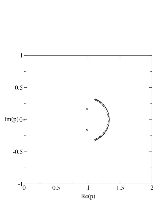
Figure 1: Singular locus ${\cal B}$ for the $L_{x}\to\infty$ limit of $sq(2\times L_{x})$ for either free, periodic, or twisted periodic longitudinal boundary conditions. For comparison, zeros of the reliability polynomial are shown for the cyclic strip with $L_{x}=30$ (i.e., $n=60$).

The locus ${\cal B}$ for the $L_{y}=2$ free strips of the square lattice, shown in Fig. 1, is formed as the continuous accumulation set of zeros of the reliability polynomial in the limit of infinite strip length, $m\to\infty$ and is the solution of the equation expressing the degeneracy of magnitudes $|\alpha_{sq,2,0,1}|=|\alpha_{sq,2,0,2}|$. This is an arc of a circle with radius 1/3 centered at 1,

$$p=1+\frac{1}{3}e^{i\theta}\quad\theta\in[-\theta_{sq2},\theta_{sq2}]$$ (5.2.11)

where

$$\theta_{sq2}={\rm arctan}(2\sqrt{2}\ )\simeq 70.53^{\circ}\ .$$ (5.2.12)

This circular arc crosses the real $p$ axis at a single point, which is thus $p_{c}$, namely

$$p_{c}=\frac{4}{3}\quad{\rm for}\quad sq,\ FBC_{y},\ 2\times\infty\ .$$ (5.2.13)

This applies here for the case of free longitudinal boundary conditions, and we shall show below that it also applies for the case of periodic or twisted periodic longitudinal boundary conditions. We find that this property that the value of $p_{c}$ for a strip of a given type of lattice and a given set of transverse boundary conditions is independent of the longitudinal boundary conditions also holds for other strips, and we indicate this when listing these values of $p_{c}$ (or $(p_{c})_{eff}$) by displaying only the transverse boundary condition ($FBC_{y}$ in eq. (5.2.13)). The arc has endpoints at the values of $p$ where the the expression $12-20p+9p^{2}$ in the square roots in $\alpha_{sq,2,0,j}$ vanishes so that $\alpha_{sq,2,0,1}=\alpha_{sq,2,0,2}$. These endpoints are

$$p=1+\frac{1}{3}e^{\pm i\theta_{sq2}}=\frac{2}{9}(5\pm\sqrt{2}\ i)\simeq 1.11111\pm 0.31427i\ .$$ (5.2.14)

Recall that two roots of an algebraic equation are equal where the discriminant vanishes; for the equation $\alpha^{2}-(4-3p)\alpha+1-p=0$ that yields $\alpha_{sq,2,0,j}$, $j=1,2$ as its roots, this discriminant is $12-20p+9p^{2}$.

5.3 $L_{y}=3$ Strip of the Square Lattice with Free Boundary Conditions

The generating function for this strip follows from our calculation of $Z(G,q,v)$ for this strip [34] and has the form (4.4.2) with

$${\cal N}=p^{2}\biggl{[}1+p^{4}(1-p)z-p^{6}(1-p)^{3}z^{2}\biggr{]}$$ (5.3.1)

and

$${\cal D}(p,z) = 1+\sum_{j=1}^{4}b_{sq3f,j}z^{j}$$ (5.3.2)

$$= \prod_{j=1}^{4}(1-p^{3}\alpha_{sq3f,j}z)$$ (5.3.4)

where

$$b_{sq3f,1}=-p^{3}(15-24p+10p^{2})$$ (5.3.5)

$$b_{sq3f,2}=p^{6}(1-p)(32-66p+46p^{2}-11p^{3})$$ (5.3.6)

$$b_{sq3f,3}=-p^{9}(1-p)^{3}(15-20p+7p^{2})$$ (5.3.7)

$$b_{sq3f,4}=p^{12}(1-p)^{5}$$ (5.3.8)

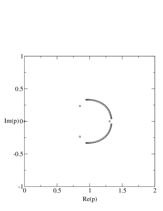
Figure 2: Singular locus ${\cal B}$ for the $L_{x}\to\infty$ limit of $sq(3\times L_{x})$ for either free, periodic, or twisted periodic longitudinal boundary conditions. For comparison, zeros of the reliability polynomial are shown for the cyclic strip of this width with $L_{x}=20$ (i.e., $n=60$).

In Fig. 2 we show the locus ${\cal B}$ for the $L_{y}=3$ strips of the square lattice with any longitudinal boundary conditions, together with zeros for the cyclic strip of this width with $L_{x}=20$. This locus consists of two complex-conjugate arcs which do not cross the real axis. From the arc endpoints closest to the real axis, one can infer the effective quantity $(p_{c})_{eff}\simeq 1.335$. The locus is again concave to the left and roughly centered about the point $p=1$.

5.4 $L_{y}=2$ Cyclic and Möbius Strips of the Square Lattice

For the reader’s convenience, we shall give some details of our calculation for this family of graphs. The Tutte polynomials for these families of graphs were computed in [29] and have $N_{T,2,\lambda}=6$, in accordance with the general formula (4.2.19). There are $n_{T}(2,0)=2$ terms with coefficient $c^{(0)}$, denoted $\lambda_{T,sq,2,0,j}$, $j=1,2$; $n_{T}(2,1)=3$ terms with coefficient $c^{(1)}$, denoted $\lambda_{T,sq,2,1,j}$, and the unique term with coefficient $c^{(2)}$, which term is $\lambda_{T,sq,2,2}=1$ as a special case of the general result (4.2.20). Explicitly,

$$T(sq[L_{y}=2,L_{x}=m,cyc],x,y)=\frac{1}{x-1}\sum_{d=0}^{2}c^{(d)}\sum_{j=1}^{n_{T}(2,d)}(\lambda_{T,sq,2,d,j})^{m}$$ (5.4.1)

(5.4.2)

$$=\frac{1}{x-1}\left[\sum_{j=1}^{2}(\lambda_{T,sq,2,0,j})^{m}+c^{(1)}\sum_{j=1}^{3}(\lambda_{T,sq,2,1,j})^{m}+c^{(2)}(\lambda_{T,sq,2,2})^{m}\right]$$ (5.4.3)

where $n_{T}(L_{y},d)$ was recalled from [32] in eq. (4.2.17) and [29]

$$\lambda_{T,sq,2,0,j}=\frac{1}{2}\biggl{[}(1+y+x+x^{2})\pm\Bigl{(}y^{2}+2y(1+x-x^{2})+(x^{2}+x+1)^{2}\Bigr{)}^{1/2}\ \biggr{]}$$ (5.4.4)

$$\lambda_{T,sq,2,1,j}=\frac{1}{2}\biggl{[}x+y+2\pm\Bigl{(}(x-y)^{2}+4(x+y+1)\Bigr{)}^{1/2}\ \biggr{]}$$ (5.4.5)

with $j=1,2$ corresponding to $\pm$, and

$$\lambda_{T,sq,2,1,3}=x\ .$$ (5.4.6)

We have discussed above how equalities occur between certain $\lambda_{T,G,L_{y},d,j}$’s when evaluated at $x=1$. We show this explicitly here. First, we have

$$\lambda_{T,sq,2,0,j}=\lambda_{T,sq,2,1,j}=\frac{1}{2}\left[y+3\pm\sqrt{y^{2}+2y+9}\ \right]\quad{\rm for}\ \ x=1$$ (5.4.7)

where $j=1,2$ refer correspond to $\pm$ on the right-hand side, respectively. Furthermore,

$$\lambda_{T,sq,2,1,3}=\lambda_{T,sq,2,2}=1\quad{\rm for}\ \ x=1\ .$$ (5.4.8)

Hence, $N_{R,sq,2,\lambda}=(1/2)N_{T,sq,2,\lambda}=3$, in accordance with the inequality (4.2.23) (realized as an equality) in our theorem above. Using L’Hopital’s rule to evaluate the Tutte polynomial (5.4.3) at $x=1$, we obtain

$$R(sq[L_{y}=2,m,cyc],p)=p^{2m}\Biggl{[}(\alpha_{sq,2,0,1})^{m}+(\alpha_{sq,2,0,2})^{m}-2(\alpha_{sq,2,2})^{m}$$ (5.4.9)

(5.4.10)

$$+mp^{-1}(1-p)^{2}\Biggl{\{}(\alpha_{sq,2,0,1})^{m-1}\left(1+\frac{3(1-p)}{\sqrt{R_{2}}}\right)$$ (5.4.11)

(5.4.12)

$$+(\alpha_{sq,2,0,2})^{m-1}\left(1-\frac{3(1-p)}{\sqrt{R_{2}}}\right)-(\alpha_{sq,2,2})^{m-1}\Biggr{\}}\Biggr{]}$$ (5.4.13)

where $R_{2}$ was defined above in eq. (5.2.5), the $\alpha_{sq,2,0,j}$ were given in (5.2.4) above, and

$$\alpha_{sq,2,2}=1-p$$ (5.4.14)

as a special case of (4.2.21) above.

For the $L_{y}=2$ Möbius (Mb) strip of the square lattice [29]

$$T(sq[L_{y}=2,L_{x}=m,Mb],x,y)=\frac{1}{x-1}\Biggl{[}\sum_{j=1}^{2}(\lambda_{T,sq,2,0,j})^{m}$$ (5.4.15)

(5.4.16)

$$+c^{(1)}\biggl{(}-(\lambda_{T,sq,2,1,1})^{m}+\sum_{j=2}^{3}(\lambda_{T,sq,2,1,j})^{m}\biggr{)}-(\lambda_{T,sq,2,2})^{m}\Biggr{]}\ .$$ (5.4.17)

From this we obtain

$$R(sq[L_{y}=2,m,Mb],p)=p^{2m}\Biggl{[}(\alpha_{sq,2,0,1})^{m}+(\alpha_{sq,2,0,2})^{m}-(\alpha_{sq,2,2})^{m}$$ (5.4.18)

(5.4.19)

$$+mp^{-1}(1-p)^{2}\Biggl{\{}(\alpha_{sq,2,0,1})^{m-1}\left(1+\frac{3(1-p)}{\sqrt{R_{2}}}\right)+(\alpha_{sq,2,0,2})^{m-1}\left(1-\frac{3(1-p)}{\sqrt{R_{2}}}\right)$$ (5.4.20)

(5.4.21)

$$+(\alpha_{sq,2,2})^{m-1}\Biggr{\}}\Biggr{]}\ .$$ (5.4.22)

For both of these $L_{y}=2$ cyclic and Möbius strips of the square lattice, the dominant term in the physical interval $p\in[0,1]$ is $\alpha_{sq,2,0,1}$ and hence the asymptotic reliability per vertex, $r$, is the same as that for the corresponding strip with free longitudinal boundary conditions, given by (5.2.8):

$$r(sq[2\times\infty,cyc.],p) = r(sq[2\times\infty,Mb.],p)$$ (5.4.23)

$$= r(sq[2\times\infty,free],p)$$ (5.4.25)

$$= r(sq[2\times\infty,FBC_{y}],p)\ .$$ (5.4.27)

For the infinite-length limit of these strip graphs, and for the respective infinite-length limits of other strip graphs to be considered below, we find that the $r$ function is independent of the longitudinal boundary conditions. This is indicated in the last line of eq. (5.4.27) and analogous equations below by listing only the type of transverse boundary condition. The dominant term for large positive $p$ is $\alpha_{sq,2,0,2}$. Because the two dominant $\alpha$’s in the reliability polynomials for these cyclic and Möbius strips are the same as the two $\alpha$’s that enter in the reliability polynomial for the corresponding strip with free boundary conditions, it follows that the locus ${\cal B}$ is identical for the $L_{y}=2$ strips of the square lattice with free, cyclic, and Möbius boundary conditions. This locus is shown in Fig. 1.

We find that the reliability polynomials $R(sq[2\times L_{x},cyc.],p)$ and $R(sq[2\times L_{x},Mb],p)$ have only $p=0$ as a real root if $L_{x}\geq 1$ is odd, while for even $L_{x}\geq 2$, they each have an additional real root. In Table 1 we list the values of this additional respective real root for the reliability polynomials of these two strips. The results in this table suggest that as $L_{x}\to\infty$, these two respective additional real zeros for the cyclic and Möbius strips could approach the same limit. The value of this limit could be about 1.3.

Table 1: Values of the real root (aside from $p=0$) of $R(sq[2\times L_{x},cyc.],p)$ and $R(sq[2\times L_{x},Mb],p)$ for even $L_{x}$.

$L_{x}$	cyc.	Mb.
2	2.000000	1.626538
4	1.404813	1.388652
6	1.349507	1.346559
8	1.333333	1.332635
10	1.327103	1.326919
12	1.324413	1.324362
14	1.323229	1.323214
16	1.322761	1.322757
18	1.322658	1.322657
20	1.322749	1.322748

5.5 $L_{y}=2$ Cylindrical Strips of the Square Lattice

This is the minimal-width strip of the square lattice with cylindrical boundary conditions and involves double vertical edges. The results for the reliability polynomial are conveniently expressed in terms of the generating function (4.4.1) and (4.4.2). We find

$${\cal N}=R(C_{2},p)=p(2-p)$$ (5.5.1)

$${\cal D} = 1-p^{2}(6-8p+3p^{2})z+(1-p)^{2}p^{4}z^{2}$$ (5.5.2)

$$= \prod_{j=1}^{2}(1-p^{2}\alpha_{sqcyl2,j}z)$$ (5.5.4)

where

$$\alpha_{sqcyl2,j}=\frac{1}{2}\left[6-8p+3p^{2}\pm\sqrt{(2-p)(4-3p)(4-6p+3p^{2})}\ \right]\ .$$ (5.5.5)

We observe that $R(sq[2\times L_{x},cyl.],p)$ always has the factor $(2-p)$; this is associated with the fact that this strip has double vertical edges. For odd $m\geq 1$, i.e., even $L_{x}\geq 2$, $R(sq[2\times L_{x},cyl.],p)$ also has the factor $(3p^{2}-8p+6)$, with roots $(1/3)(4\pm\sqrt{2}i)$. For $m\geq 4$, we observe that $R(sq[2\times L_{x},cyl.],p)$ has, besides the real zeros at $p=0,2$, a set of real zeros in the interval $(1,2]$. Among other features, we note that as $m$ increases, (i) the number of real zeros in this interval increases; (ii) the smallest zero in this interval decreases monotonically toward 4/3; (iii) the largest zero increases monotonically toward 2 as $m$ increases, and (iv) the density of zeros is largest in the regions slightly above 4/3 and slightly below 2. A plot of these zeros is shown in Fig. 3; as is evident from this plot, as $m\to\infty$, these real zeros away from $p=0$ accumulate to form the line segment on ${\cal B}$ extending between $p=4/3$ and $p=2$.

In the physical interval $p\in[0,1]$ the dominant term is $\alpha_{sqcyl2,1}$, so the asymptotic reliability per vertex is

$$r(sq[2\times\infty,PBC_{y}],p)=p(\alpha_{sqcyl2,1})^{1/2}$$ (5.5.6)

$$= \frac{p}{\sqrt{2}}\left[6-8p+3p^{2}+\sqrt{(2-p)(4-3p)(4-6p+3p^{2})}\ \right]^{1/2}$$ (5.5.8)

This has derivatives

$$\left.\frac{dr}{dp}\right|_{p=0}=1+\sqrt{2}=2.41421...$$ (5.5.9)

and $dr/dp=0$ at $p=1$.

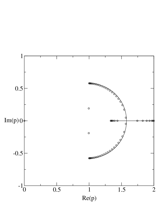
Figure 3: Singular locus ${\cal B}$ for the $L_{x}\to\infty$ limit of $sqcyl(2\times L_{x})$ for either free or (twisted) periodic longitudinal boundary conditions. For comparison, zeros of the reliability polynomial are shown for the torus strip with $L_{x}=30$ (i.e., $n=60$).

The locus ${\cal B}$, shown in Fig. 3, is given by the union of an arc of a circle with a line segment on the real axis:

$${\cal B}:\quad\{p=1+\frac{1}{\sqrt{3}}e^{i\theta}\ ,\quad\theta\in[-\pi/2,\pi/2]\}\ \cup\{\frac{4}{3}\leq p\leq 2\}\ .$$ (5.5.10)

Hence,

$$p_{c}=2\quad{\rm for}\quad sq,\ PBC_{y},\ 2\times\infty$$ (5.5.11)

The circular arc intersects the real axis and line segment at $p=1+\frac{1}{\sqrt{3}}\simeq 1.577$. The endpoints of the arc are located at

$$p_{sqce},p_{sqce}^{*}=1\pm\frac{i}{\sqrt{3}}$$ (5.5.12)

These points, together with the endpoints of the line segment, $p=4/3$ and $p=2$ are the zeros of the expression in the square root in $\alpha_{sqcyl2,j}$ in eq. (5.5.5), which expression is the discriminant of the equation $\alpha^{2}-(6-8p+3p^{2})\alpha+(1-p)^{2}=0$ whose roots are these $\alpha$’s.

5.6 $L_{y}=2$ Torus and Klein Bottle Strips of the Square Lattice

Either using a direct calculation or as a special case of our previous calculation of the Tutte polynomial [33], using (3.2), we find

$$R(sq[L_{y}=2,m,torus],p)=p^{2m}\Biggl{[}(\alpha_{sqtor2,1})^{m}+(\alpha_{sqtor2,2})^{m}-2(\alpha_{sqtor2,3})^{m}$$ (5.6.1)

(5.6.2)

$$-mp^{-1}(1-p)^{2}\left\{\frac{(\alpha_{sqtor2,1})^{m-1}}{2}\left(2p-3+\frac{(p-2)(6p^{2}-13p+8)}{\sqrt{(p-2)(3p-4)(3p^{2}-6p+4)}}\right)\right.$$ (5.6.3)

(5.6.4)

$$\left.+\frac{(\alpha_{sqtor2,2})^{m-1}}{2}\left(2p-3-\frac{(p-2)(6p^{2}-13p+8)}{\sqrt{(p-2)(3p-4)(3p^{2}-6p+4}}\right)+(1-p)(\alpha_{sqtor2,3})^{m-1}\right\}\Biggr{]}$$ (5.6.5)

(5.6.6)

(5.6.7)

where

$$\alpha_{sqtor2,j}=\alpha_{sqcyl2,j}\quad j=1,2$$ (5.6.8)

with $\alpha_{sqcyl2,j}$, $j=1,2$, given above in (5.5.5) and,

$$\alpha_{sqtor2,3}=(1-p)^{2}\ .$$ (5.6.9)

For the $L_{y}=2$ Klein bottle (Kb.) strip of the square lattice

$$R(sq[L_{y}=2,m,Kb.],p)=p^{2m}\Biggl{[}(\alpha_{sqtor2,1})^{m}+(\alpha_{sqtor2,2})^{m}-(\alpha_{sqtor2,3})^{m}$$ (5.6.10)

(5.6.11)

$$-mp^{-1}(1-p)^{2}\left\{\frac{(\alpha_{sqtor2,1})^{m-1}}{2}\left(2p-3+\frac{(p-2)(6p^{2}-13p+8)}{\sqrt{(p-2)(3p-4)(3p^{2}-6p+4)}}\right)\right.$$ (5.6.12)

(5.6.13)

$$\left.+\frac{(\alpha_{sqtor2,2})^{m-1}}{2}\left(2p-3-\frac{(p-2)(6p^{2}-13p+8)}{\sqrt{(p-2)(3p-4)(3p^{2}-6p+4)}}\right)-(1-p)(\alpha_{sqtor2,3})^{m-1}\right\}\Biggr{]}$$ (5.6.14)

(5.6.15)

(5.6.16)

In the physical region $p\in[0,1]$, the dominant term is $\alpha_{sqtor2,1}$ for both of these families of strips, and hence $r(sq[2\times\infty,torus/Kb.],p)=r(sq[2\times\infty,cyl.],p)$. This equality has already been incorporated in our notation $r(sq[2\times\infty,PBC_{y}],p)$ in eq. (5.5.8). This is another example of the feature that for a given type of strip graph $G_{s}$ with a given width and set of transverse boundary conditions, $r$ is independent of the longitudinal boundary conditions.

Similarly, since the locus ${\cal B}$ is determined by the equality in magnitude of the two dominant eigenvalues $\alpha_{sqtor2,1}$ and $\alpha_{sqtor2,2}$, and since these are the same for the corresponding strip with cylindrical boundary conditions, it follows that this locus is the same as the locus for the $L_{y}=2$ cylindrical strip of the square lattice, shown in Fig. 3.

5.7 $L_{y}=3$ Cylindrical Strips of the Square Lattice

Again we express the results in terms of the generating function for the reliability polynomial, (4.4.1) and (4.4.2). We find

$${\cal N}=R(C_{3},p)+p^{5}(3-p)(1-p)^{2}z=p^{2}[3-2p+p^{3}(3-p)(1-p)^{2}z]$$ (5.7.1)

where $R(C_{3},p)=p^{2}(3-2p)$, and

$${\cal D} = 1-p^{3}(24-56p+46p^{2}-13p^{3})z+p^{6}(1-p)^{2}(24-46p+30p^{2}-7p^{3})z^{2}-p^{9}(1-p)^{5}z^{3}$$ (5.7.2)

$$= \prod_{j=1}^{3}(1-p^{3}\alpha_{sqcyl3,j}z)\ .$$ (5.7.4)

The largest of the roots of the associated equation

$$\xi^{3}-(24-56p+46p^{2}-13p^{3})\xi^{2}$$ (5.7.5)

(5.7.6)

$$+(1-p)^{2}(24-46p+30p^{2}-7p^{3})\xi-(1-p)^{5}=0$$ (5.7.7)

is the dominant $\alpha_{sqcyl3,max}$, so that

$$r(sq[3\times\infty,PBC_{y}],p)=p(\alpha_{sqcyl3,max})^{1/3}\ .$$ (5.7.8)

This function has the property that $dr/dp=2.84207...$ at $p=0$ and $dr/dp=0$ at $p=1$. We find that the reliability polynomial $R(sq[3\times\infty,cyl.],p)$ has only $p=0$ as a real root if $m\geq 1$ is odd, i.e. $L_{x}\geq 2$ is even, while for even $m\geq 0$, i.e., odd $L_{x}\geq 1$, it has an additional real root which decreases as $m$ increases and appears to approach a limit of roughly 1.4. In Table 2 we list the values of this additional real root.

Table 2: Values of the real root (aside from $p=0$) of $R(sq[3\times\infty,cyl.],p)$ for odd $L_{x}$.

$L_{x}$	root
1	1.500000
3	1.440337
5	1.422909
7	1.416297
9	1.412887
11	1.410809
13	1.409409
15	1.408403
17	1.407644
19	1.407051
21	1.406575

Figure 4: Singular locus ${\cal B}$ for the $L_{x}\to\infty$ limit of $sqcyl(3\times L_{x})$ for either free or (twisted) periodic longitudinal boundary conditions. For comparison, zeros of the reliability polynomial are shown for the toroidal strip with $L_{x}=20$ (i.e., $n=60$).

In Fig. 4 we show a plot of ${\cal B}$ for the $L_{x}\to\infty$ limit of the $L_{y}=3$ strip of the square lattice with cylindrical boundary conditions.

5.8 $L_{y}=4$ Cylindrical Strip of the Square Lattice

As before, we express the results for the $L_{y}=4$ strip of the square lattice with cylindrical boundary conditions in terms of the numerator and denominator of the generating function. In particular, for the denominator, we find

$${\cal D} = 1+\sum_{j=1}^{6}b_{sqcyl4,j}z^{j}$$ (5.8.1)

$$= \prod_{j=1}^{6}(1-p^{4}\alpha_{sqcyl4,j}z)$$ (5.8.3)

where

$$b_{sqcyl4,1}=-p^{4}(90-293p+369p^{2}-211p^{3}+46p^{4})$$ (5.8.4)

$$b_{sqcyl4,2}=p^{8}(1-p)^{2}(735-2977p+5094p^{2}-4710p^{3}+2481p^{4}-706p^{5}+85p^{6})$$ (5.8.5)

$$b_{sqcyl4,3} = -p^{12}(1-p)^{4}(1548-7518p+15948p^{2}-19170p^{3}$$ (5.8.8)

$$+14104p^{4}-6351p^{5}+1621p^{6}-181p^{7})$$

$$b_{sqcyl4,4}=p^{16}(1-p)^{7}(735-3177p+5870p^{2}-5934p^{3}+3456p^{4}-1097p^{5}+148p^{6})$$ (5.8.9)

$$b_{sqcyl4,5}=-p^{20}(1-p)^{11}(90-223p+208p^{2}-88p^{3}+15p^{4})$$ (5.8.10)

$$b_{sqcyl4,6}=p^{24}(1-p)^{15}$$ (5.8.11)

The degree of ${\cal D}$ is too high to obtain closed-form algebraic expressions for the $\alpha_{sqcyl4,j}$’s, but they may be computed numerically. Denoting the dominant $\alpha_{sqcyl4,j}$ in the physical interval $p\in[0,1]$ as $\alpha_{sqcyl4,max}$, one has, for the asymptotic reliability per vertex, $r(sq[4\times\infty,PBC_{y}],p)=p(\alpha_{sqcyl4,max})^{1/4}$. In Fig. 5 we show the locus ${\cal B}$ for the infinite-length limit of this strip. This locus includes two complex-conjugates arcs, a self-conjugate arc crossing the real axis at $p\simeq 1.364$, and a real line segment extending from $p=4/3$ to $p\simeq 1.384$, which defines the value of $p_{c}$ for this strip.

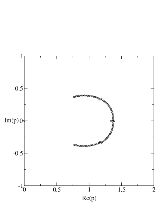
Figure 5: Singular locus ${\cal B}$ for the $L_{x}\to\infty$ limit of $sqcyl(4\times L_{x})$ for either free or (twisted) periodic longitudinal boundary conditions. For comparison, zeros of the reliability polynomial are shown for the cylindrical strip with $L_{x}=21$ (i.e., $n=84$).

5.9 $L_{y}=2$ Strip of the Triangular Lattice with Free Boundary Conditions

In addition to studying how reliability polynomials and their asymptotic $r$ functions depend on the width and boundary conditions, it is also of interest to explore how they depend on the lattice type. For this purpose we have carried out calculations of reliability polynomials for strips of the triangular and honeycomb lattice. We begin with the $L_{y}=2$ strip of the triangular lattice with free boundary conditions, for which we calculate the generating function with

$${\cal N}(p,z)=p\biggl{[}1+p(1-p)z\biggr{]}$$ (5.9.1)

$${\cal D}(p,z) = 1-p^{2}(7-10p+4p^{2})z+p^{4}(1-p)^{2}z^{2}$$ (5.9.2)

$$= (1-p^{2}\alpha_{t,2,0,1}z)(1-p^{2}\alpha_{t,2,0,2}z)$$ (5.9.4)

where

$$\alpha_{t,2,0,j} = \frac{1}{2}\left[7-10p+4p^{2}\pm(3-2p)\sqrt{5-8p+4p^{2}}\right]$$ (5.9.5)

$$= \left[\frac{3-2p+\sqrt{5-8p+4p^{2}}}{2}\right]^{2}\quad{\rm for}\quad j=1,2\ .$$ (5.9.7)

We note that $R(p,z)$ for the strip of the triangular lattice of length $m$ has the factor $(8-11p+4p^{2})$ if $m=1$ mod 3, where our convention is that $m=1$ is a single square with diagonal (i.e. two triangles), and so forth.

The dominant term in the physical interval $p\in[0,1]$ is $\alpha_{t,2,0,1}$, and hence the reliability per vertex for $L_{x}\to\infty$ is

$$r(t[2\times\infty,FBC_{y}],p) = p(\alpha_{t,2,0,1})^{1/2}$$ (5.9.8)

$$= \frac{p}{\sqrt{2}}\left[7-10p+4p^{2}\pm(3-2p)\sqrt{5-8p+4p^{2}}\right]^{1/2}$$ (5.9.10)

This has derivatives

$$\left.\frac{dr}{dp}\right|_{p=0}=\frac{3+\sqrt{5}}{2}=2.61803...$$ (5.9.11)

and $dr/dp=0$ at $p=1$.

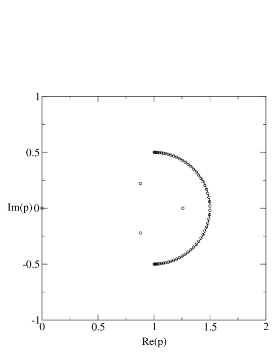
Figure 6: Singular locus ${\cal B}$ for the $L_{x}\to\infty$ limit of $tri(2\times L_{x})$ for either free or (twisted) periodic longitudinal boundary conditions. For comparison, zeros of the reliability polynomial are shown for the cyclic strip with $L_{x}=30$ (i.e., $n=60$).

The locus ${\cal B}$, shown in Fig. 6, is given by an arc of a circle:

$${\cal B}:\quad p=1+\frac{1}{2}e^{i\theta}\ ,\quad\theta\in[-\frac{\pi}{2},\frac{\pi}{2}]$$ (5.9.12)

This is a leftwardly concave circular arc that crosses the real axis at

$$p_{c}=\frac{3}{2}\quad tri,\ FBC_{y},\ 2\times\infty,$$ (5.9.13)

and has endpoints at $p=1\pm i/2$, where the factor $5-8p+4p^{2}$ in the discriminant $(5-8p+4p^{2})(3-2p)^{2}$ of the equation $\alpha^{2}-(7-10p+4p^{2})\alpha+(1-p)^{2}=0$ yielding the $\alpha$’s vanishes. We shall see that a rather different strip, the self-dual strip of the square lattice of width $L_{y}=1$, yields the same locus ${\cal B}$, although the reliability polynomials are different. Interestingly, the effective degree is the same, namely 4, for these two strips, although the $L_{y}=2$ cyclic strip of the triangular lattice is a $\Delta$-regular graph, with uniform vertex degree $\Delta=4$, whereas the self-dual strip of the square lattice with $L_{y}=1$ has two quite different kinds of vertex degrees - 3 for the outer rim and $m$ for the central vertex connected to each vertex on the rim by edges. However, it is not, in general, true that if two families of graphs have the same effective vertex degree then the resultant loci ${\cal B}$ are the same; for example, each of the self-dual cyclic strips of the square lattice of width $L_{y}$ has the same effective vertex degree in the limit $L_{x}\to\infty$, but they have different loci ${\cal B}$.

5.10 $L_{y}=2$ Cyclic Strip of the Triangular Lattice

We next consider the $L_{y}=2$ cyclic strip of the triangular lattice. Either using a direct calculation or as a special case of our previous calculation of the Tutte polynomial [30], using (3.2), we find

$$R(t[L_{y}=2,m,cyc],p)=p^{2m}\Biggl{[}(\alpha_{t,2,0,1})^{m}+(\alpha_{t,2,0,2})^{m}-2(\alpha_{t,2,2})^{m}$$ (5.10.1)

(5.10.2)

$$+mp^{-1}(5-3p)^{-1}(1-p)^{2}\left\{(\alpha_{t,2,0,1})^{m-1}(1-p)\left(7-4p+\frac{(3-2p)(5-4p)}{\sqrt{4p^{2}-8p+5}}\right)\right.$$ (5.10.3)

(5.10.4)

$$+\left.(\alpha_{t,2,0,2})^{m-1}(1-p)\left(7-4p-\frac{(3-2p)(5-4p)}{\sqrt{4p^{2}-8p+5}}\right)-2(p^{2}-3p+2)(\alpha_{t,2,2})^{m-1}\right\}\Biggr{]}$$ (5.10.5)

(5.10.6)

(5.10.7)

where $\alpha_{t,2,0,j}$ were given above for the free strip and

$$\alpha_{t,2,2}=(1-p)^{2}\ .$$ (5.10.8)

Because the dominant $\alpha$’s consist of $\alpha_{t,2,0,j}$, $j=1,2$, which are the same for the free, cyclic, and Möbius strips, it follows that the locus ${\cal B}$ is the same for the $L_{x}\to\infty$ limits of these three strips.

5.11 $L_{y}=2$ Free Strips of the Honeycomb Lattice

For the $L_{y}=2$ strip of the honeycomb lattice with free boundary conditions we calculate a generating function with

$${\cal N}=p$$ (5.11.1)

$${\cal D} = 1-p^{4}(6-5p)z+(1-p)p^{8}z^{2}$$ (5.11.2)

$$= (1-p^{4}\alpha_{hc,2,0,1}z)(1-p^{4}\alpha_{hc,2,0,2}z)$$ (5.11.4)

where

$$\alpha_{hc,2,0,j}=\frac{1}{2}\left[6-5p\pm\sqrt{H_{2}}\ \right]$$ (5.11.5)

with

$$H_{2}=32-56p+25p^{2}\ .$$ (5.11.6)

In the physical interval $p\in[0,1]$ the dominant term is $\alpha_{hc,2,0,1}$, so the asymptotic reliability per vertex is

$$r(hc[2\times\infty,FBC_{y}],p) = p(\alpha_{hc,2,0,1})^{1/4}$$ (5.11.7)

$$= \frac{p}{2^{1/4}}\left[6-5p+\sqrt{32-56p+25p^{2}}\right]^{1/4}$$ (5.11.9)

This has derivatives

$$\left.\frac{dr}{dp}\right|_{p=0}=(1+\sqrt{2})^{1/2}=1.55377...$$ (5.11.10)

and $dr/dp=0$ at $p=1$.

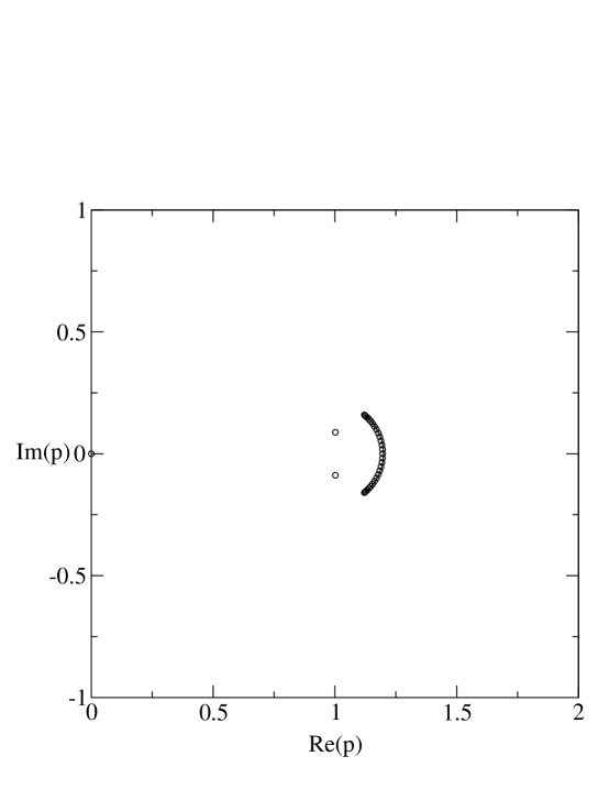
Figure 7: Singular locus ${\cal B}$ for the $L_{x}\to\infty$ limit of $hc(2\times L_{x})$ for either free or (twisted) periodic longitudinal boundary conditions. For comparison, zeros of the reliability polynomial are shown for the cyclic strip with $L_{x}=30$ (i.e., $n=120$).

The locus ${\cal B}$, shown in Fig. 7, is given by an arc of a circle:

$${\cal B}:\quad p=1+\frac{1}{5}e^{i\theta}\ ,\quad\theta\in[-\theta_{hce},\theta_{hce}]$$ (5.11.11)

where

$$\theta_{hce}={\rm arctan}(4/3)\simeq 53.13^{\circ}$$ (5.11.12)

This is a leftwardly concave arc that crosses the real axis at

$$p_{c}=\frac{6}{5}\quad{\rm for}\quad hc,\ FBC_{y},\ 2\times\infty,$$ (5.11.13)

and has endpoints at

$$p_{hce},p_{hce}^{*}=\frac{4}{25}(7\pm i)$$ (5.11.14)

where the discriminant $H_{2}$ vanishes.

5.12 $L_{y}=2$ Cyclic and Möbius Strips of the Honeycomb Lattice

For the $L_{y}=2$ cyclic strip of the honeycomb lattice, either using a direct calculation or as a special case of our previous calculation of the Tutte polynomial [33], using (3.2), we find

$$R(hc[L_{y}=2,m,cyc],p)=p^{4m}\Biggl{[}(\alpha_{hc,2,0,1})^{m}+(\alpha_{hc,2,0,2})^{m}-2(\alpha_{hc,2,2})^{m}$$ (5.12.1)

(5.12.2)

$$+mp^{-1}(1-p)^{2}\left\{(\alpha_{hc,2,0,1})^{m-1}\left(3+\frac{16-15p}{\sqrt{H_{2}}}\right)\right.$$ (5.12.3)

(5.12.4)

$$\left.+(\alpha_{hc,2,0,2})^{m-1}\left(3-\frac{16-15p}{\sqrt{H_{2}}}\right)-2(\alpha_{hc,2,2})^{m-1}\right\}\Biggr{]}$$ (5.12.5)

(5.12.6)

(5.12.7)

where $\alpha_{hc,2,0,j}$, $j=1,2$, were given above in (5.11.5) and, as a special case of (4.2.21), we have

$$\alpha_{hc,2,2}=1-p\ .$$ (5.12.8)

For the $L_{y}=2$ Möbius strip of the honeycomb lattice, using the same methods, we obtain

$$R(hc[L_{y}=2,m,Mb],p)=p^{4m}\Biggl{[}(\alpha_{hc,2,0,1})^{m}+(\alpha_{hc,2,0,2})^{m}-(\alpha_{hc,2,2})^{m}$$ (5.12.9)

(5.12.10)

$$+mp^{-1}(1-p)^{2}\left\{(\alpha_{hc,2,0,1})^{m-1}\left(3+\frac{16-15p}{\sqrt{H_{2}}}\right)\right.$$ (5.12.11)

(5.12.12)

$$\left.+(\alpha_{hc,2,0,2})^{m-1}\left(3-\frac{16-15p}{\sqrt{H_{2}}}\right)+2(\alpha_{hc,2,2})^{m-1}\right\}\Biggr{]}\ .$$ (5.12.13)

(5.12.14)

(5.12.15)

Since the locus ${\cal B}$ is determined by the equality in magnitude of the two dominant eigenvalues $\alpha_{hc,2,0,1}$ and $\alpha_{hc,2,0,2}$, and since these are the same for the strip with free and periodic or twisted periodic boundary conditions, it follows that this locus is the same as (5.11.11) and (5.11.12) for the $L_{y}=2$ cyclic or Möbius strip of the honeycomb lattice. We show this locus in Fig. 7.

5.13 $L_{y}=1$ Cyclic Strip of the Square Lattice with Self-Dual Boundary Conditions

We have presented some general structural results above for reliability polynomials of cyclic strip graphs of the square lattice with self-dual boundary conditions. Recall that these are denoted $G_{D}$, of size $L_{y}\times L_{x}$; in subscripts we will use the symbol $sqdbc$. In this and the next section we give explicit calculations of the reliability polynomials. Note that $G_{D}[1\times L_{x}]$ is the wheel graph with a central spoke vertex connected to $L_{x}$ outer vertices on the rim. Either using a direct calculation or as a special case of our previous calculation of the Tutte polynomial [36, 37], using (3.2), we find (with $L_{x}=m$)

$$R(G_{D}[1\times m],p)=p^{m}\biggl{[}(\alpha_{sqdbc,1,1,1})^{m}+(\alpha_{sqdbc,1,1,2})^{m}-2(\alpha_{sqdbc,1,2,1})^{m}\biggr{]}$$ (5.13.1)

where

$$\alpha_{sqdbc,1,1,j}=\frac{1}{2}\biggl{[}3-2p\pm\sqrt{5-8p+4p^{2}}\ \biggr{]}\quad j=1,2$$ (5.13.2)

and, consistent with (4.2.21),

$$\alpha_{sqdbc,1,2,1}=1-p\ .$$ (5.13.3)

In accordance with our general results above, the total number of terms is the same as that for the Tutte polynomial, $N_{R,G_{D},L_{y}=1,\lambda}=N_{T,G_{D},L_{y}=1,\lambda}=3$.

In the physical interval $p\in[0,1]$ the dominant term is $\alpha_{sqdbc,1,1,1}$ so that the asymptotic reliability per vertex is

$$r(G_{D}[1\times\infty],p) = p\alpha_{sqdbc,1,1,1}$$ (5.13.4)

$$= p\left[\ \frac{3-2p+\sqrt{5-8p+4p^{2}}}{2}\ \right]$$ (5.13.6)

Interestingly, although the graphs are different and the reliability polynomials are different for the $G_{D}(1\times m)$ and $tri(2\times m)$ strips (with either both free or both periodic longitudinal boundary conditions), the infinite-length limits of these four families of graphs yield the same $r$ function, i.e., (5.13.6) is identical to $r(tri[2\times\infty,FBC_{y}],p)$ given above in (5.9.10).

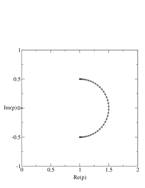
Figure 8: Singular locus ${\cal B}$ for the $L_{x}\to\infty$ limit of $G_{D}(1\times L_{x})$. For comparison, zeros of the reliability polynomial are shown for $L_{x}=40$.

The locus ${\cal B}$ is shown in Fig. 8 and forms arc of a circle centered at $p=1$ of radius 1/2 with endpoints at $p=1\pm(1/2)i$, i.e.,

$${\cal B}:\quad p=1+\frac{1}{2}e^{i\theta}\ ,\quad\theta\in[-\frac{\pi}{2},\frac{\pi}{2}]$$ (5.13.7)

so that

$$p_{c}=\frac{3}{2}\quad{\rm for}\quad G_{D}(1\times\infty)\ .$$ (5.13.8)

The endpoints occur at the branch point singularities of the polynomial $5-8p+4p^{2}$ that appears in the square root in the terms (5.13.2). The locus (5.13.7) is identical to (5.9.12), although the $\alpha$’s involved are different.

5.14 $L_{y}=2$ Cyclic Strip of the Square Lattice with Self-Dual Boundary Conditions

For $G_{D}[2\times m]$, our general formulas give $N_{R,G_{D},2,\lambda}=10$ with $n_{R}(G_{D},2,1)=5$, $n_{R}(G_{D},2,2)=4$, and $n_{R}(G_{D},2,3)=1$. We find that $R(G_{D}[2\times m],p)$ has the form (4.3.4),

$$R(G_{D}[2\times m],p)=p^{2m}\biggl{[}\sum_{j=1}^{5}(\alpha_{sqdbc,2,1,j})^{m}-2\sum_{j=1}^{4}(\alpha_{sqdbc,2,2,j})^{m}+3(\alpha_{sqdbc,2,3,1})^{m}\biggr{]}$$ (5.14.1)

where

$$\alpha_{sqdbc,2,3,1}=(1-p)^{2}$$ (5.14.2)

and the $\alpha_{sqdbc,2,2,j}$ are the roots of the degree-4 equation

$$\xi^{4}+a_{db1}\xi^{3}+a_{db2}\xi^{2}+a_{db3}\xi+a_{db4}=0$$ (5.14.3)

with

$$a_{db1}=-(1-p)(7-5p)$$ (5.14.4)

$$a_{db2}=(1-p)^{2}(13-17p+5p^{2})$$ (5.14.5)

$$a_{db3}=-(1-p)^{4}(7-5p)$$ (5.14.6)

$$a_{db4}=(1-p)^{6}\ .$$ (5.14.7)

In eq. (5.14.1) the $\alpha_{sqdbc,2,1,j}$ are the roots of the degree-5 equation

$$\xi^{5}+b_{db1}\xi^{4}+b_{db2}\xi^{3}+b_{db3}\xi^{2}+b_{db4}\xi+b_{db5}=0$$ (5.14.8)

where

$$b_{db1}=-(12-18p+7p^{2})$$ (5.14.9)

$$b_{db2}=(1-p)(36-67p+41p^{2}-8p^{3})$$ (5.14.10)

$$b_{db3}=-(1-p)^{2}(36-75p+53p^{2}-13p^{3})$$ (5.14.11)

$$b_{db4}=2(1-p)^{4}(3-2p)(2-p)$$ (5.14.12)

$$b_{db5}=-(1-p)^{6}\ .$$ (5.14.13)

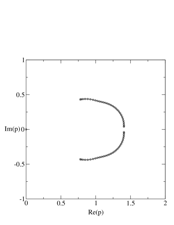
Figure 9: Singular locus ${\cal B}$ for the $L_{x}\to\infty$ limit of $G_{D}(2\times L_{x})$. For comparison, zeros of the reliability polynomial are shown for $L_{x}=30$ (i.e., $n=61$).

The locus ${\cal B}$ is shown in Fig. 9 and consists of arcs, again concave to the left, that almost cross, but actually have endpoints near to, the real axis at $q\simeq 1.4$ and have endpoints at $q\simeq 0.7765\pm 0.4302i$ and $q\simeq 1.406\pm 0.036795i$.

5.15 $L_{y}=3$ Cyclic Strip of the Square Lattice with Self-Dual Boundary Conditions

For $G_{D}[3\times m]$, our general formulas give $N_{R,G_{D},3,\lambda}=35$ with $n_{R}(G_{D},3,4)=1$, $n_{R}(G_{D},3,3)=6$, $n_{R}(G_{D},3,2)=14$, and $n_{R}(G_{D},3,1)=14$. We have calculated the reliability polynomial from our earlier calculation of the Tutte polynomial for this strip [37, 38]. Since the results for the $\alpha$’s are rather complicated, we do not list them in detail here (some examples are given in the appendix) but instead concentrate on the locus ${\cal B}$. This is shown in Fig. 10.

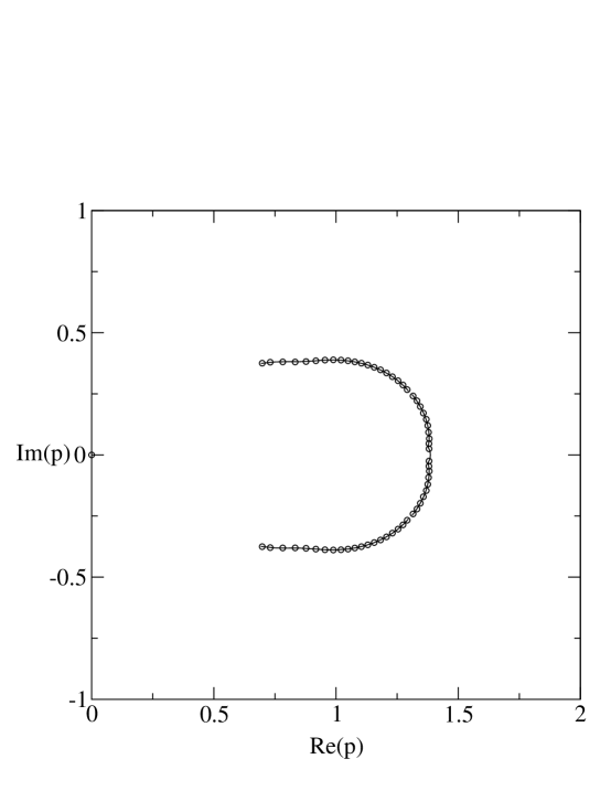
Figure 10: Singular locus ${\cal B}$ for the $L_{x}\to\infty$ limit of $G_{D}(3\times L_{x})$. For comparison, zeros of the reliability polynomial are shown for $L_{x}=20$ (i.e., $n=61$).

5.16 Some Families of Graphs with Multiple Edges

Consider a connected graph $G=(V,E)$. We take this graph to be loopless; this incurs no loss of generality since loops do not affect the reliability polynomial. Now consider a graph $H$ obtained from $G$ by adding another edge. Clearly, for the physical range $p\in[0,1]$, the inequality $R(H,p)\geq R(G,p)$ holds, with equality only at $p=1$. That is, adding further communications link(s) between two (already connected) nodes in a network increases the reliability of the network. A particularly simple modification in the graph is to replace each edge joining two vertices by $\ell$ edges joining these edges, thereby obtaining what we have denoted $G_{\ell}$ above. Given any such graph $G$, whether or not it is a member of a recursive family, our theorem above with (4.5.1) and (4.5.2) enables one to calculate $R(G_{\ell},p)$. Here we shall present some illustrations of this. For definiteness, we consider the $L_{y}=2$ cyclic strip of the square lattice. Using our calculation of the reliability polynomial for the $L_{y}=2$ strip of the square lattice together with our theorem, we have calculated the reliability polynomial for the same strip with all edges replaced by $\ell$-fold multiple edges joining the same vertices.

We have calculated the loci ${\cal B}$ in the $L_{x}\to\infty$ limit for these strips. The single point at $p=4/3$ where the locus ${\cal B}$ crosses the real $p$ axis for the $sq[2\times\infty]$ case, shown in Fig. 1, corresponds to $\ell$ separate points for the $\ell$-fold edge replication of $sq[2\times\infty]$. These can be calculated using (4.5.1) with (4.5.2), and we obtain

$$p=1-\frac{1}{3^{1/\ell}}e^{\frac{i\pi(1+2k)}{\ell}}\ ,\quad k=0,1,...,\ell-1$$ (5.16.1)

For example, for $\ell=2$, this yields the two values $p=1\pm i/\sqrt{3}$, and so forth for higher values of $\ell$. The arc endpoints can be calculated in the same way.

It is also of interest to study strip graphs in which a certain subset of the edges are replaced by $\ell$-fold replicated edges joining the same vertices. A simple example of this is already provided by the $L_{y}=2$ strips of the square lattice with cylindrical, torus, or Klein bottle boundary conditions, which have double transverse edges. We have calculated the reliability polynomials for the cyclic $L_{y}=2$ strips of the square lattice with $\ell$-fold multiple transverse edges. We denote these strip graphs as $sq[2\times m,cyc.,v\ell]$. We find

$$R(sq[L_{y}=2,m,cyc,v\ell],p)=p^{2m}\Biggl{[}(\alpha_{sqcyc2,v\ell,1})^{m}+(\alpha_{sqcyc2,v\ell,2})^{m}-2(\alpha_{sqcyc2,v\ell,3})^{m}$$ (5.16.2)

(5.16.3)

$$+mp^{-1}(1-p)^{\ell+1}\left\{(\alpha_{sqcyc2,v\ell,1})^{m-1}\left(VL1(p,\ell)+VL2(p,\ell)\right)\right.$$ (5.16.4)

(5.16.5)

$$\left.+(\alpha_{sqcyc2,v\ell,2})^{m-1}\left(VL1(p,\ell)-VL2(p,\ell)\right)-(\alpha_{sqcyc2,v\ell,3})^{m-1}\right\}\Biggr{]}$$ (5.16.6)

(5.16.7)

(5.16.8)

where

$$\alpha_{sqcyc2,v\ell,j}=(2p)^{-1}\Biggl{[}2-p-(2-3p)(1-p)^{\ell}$$ (5.16.9)

(5.16.10)

$$\pm[(1-(1-p)^{\ell})((2-p)^{2}-(2-3p)^{2}(1-p)^{\ell})]^{1/2}\Biggr{]},\quad j=1,2$$ (5.16.11)

$$\alpha_{sqcyc2,v\ell,3}=(1-p)^{\ell}$$ (5.16.12)

and

$$VL1(p,\ell)=\frac{(1-p)^{\ell-1}(2p-1)+1}{2p(1-p)^{\ell-1}}$$ (5.16.13)

$$VL2(p,\ell)=\frac{(2p-1)(3p-2)(1-p)^{\ell}-4+10p-7p^{2}+\frac{2-p}{(1-p)^{\ell-1}}}{2p[(1-(1-p)^{\ell})((2-p)^{2}-(2-3p)^{2}(1-p)^{\ell})]^{1/2}}$$ (5.16.14)

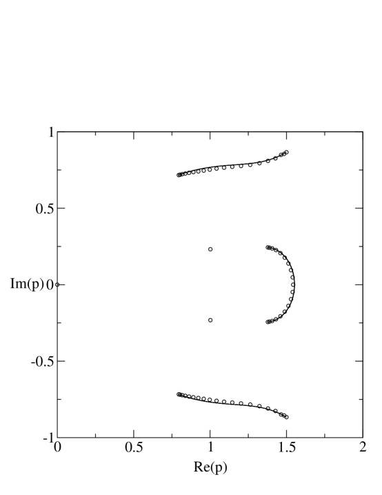
Figure 11: Singular locus ${\cal B}$ for the $L_{x}\to\infty$ limit of the $L_{y}=2$ strip of the square lattice with $\ell=3$-fold multiple transverse edges. For comparison, zeros of the reliability polynomial are shown for this strip with cyclic boundary conditions and $L_{x}=20$.

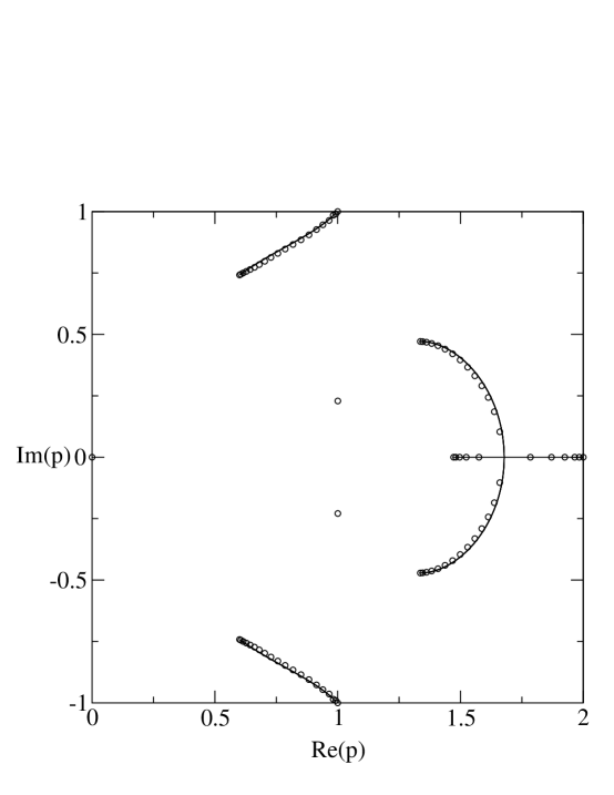
Figure 12: Singular locus ${\cal B}$ for the $L_{x}\to\infty$ limit of the $L_{y}=2$ strip of the square lattice with $\ell=4$-fold multiple transverse edges. For comparison, zeros of the reliability polynomial are shown for this strip with cyclic boundary conditions and $L_{x}=20$.

In Figs. 11 and 12 we show the loci ${\cal B}$ in the limit $L_{x}\to\infty$ for the cases $\ell=3,4$. In general, ${\cal B}$ contains arcs protruding inward from points on the circle $|p-1|=1$ given by $p=1-\exp(2i\pi k/\ell)$ (cf. eq. (4.5.7)) for $0\leq k\leq\ell-1$. If and only if $\ell$ is even, then one of these points, namely the one corresponding to $k=\ell/2$, occurs at $p=2$, and the part of ${\cal B}$ that connects with this point is a line segment on the real axis extending from $p=2$ downward to an $\ell$-dependent lower limit.

5.17 $L_{y}=2$ Free Strip of the $sq_{d}$ Lattice with Multiple Transverse Edges

In this section we exhibit the first of several recursive families of lattice strip graphs that we have found with the property that some zeros of their reliability polynomials and, in the limit of infinite length, some portions of their accumulation sets ${\cal B}$, lie outside the disk $|p-1|$. This family is a one-parameter family generalizing the lowest-order graph found by Royle and Sokal. That graph is constructed as follows [20]: start with the complete graph $K_{4}$ and choose two nonintersecting edges; replace each of these edges by six edges in parallel, i.e., joining the same pair of vertices. (Here the complete graph $K_{n}$ is defined as the graph with $n$ vertices such that every vertex is connected by one edge to every other vertex.) We had previously calculated Tutte and chromatic polynomials for strips composed of $K_{4}$ subgraphs [52, 51, 35]. One of the equivalent ways of defining these strip graphs is to start with a strip of the square lattice and add edges connecting diagonally opposite vertices of each square, thereby replacing each square by a $K_{4}$; they were thus denoted strips of the $sq_{d}$ lattice, $sq_{d}(2\times L_{x},BC_{x})$, where $BC_{x}$ indicated the longitudinal boundary conditions. In a physical context, the Potts model on the $sq_{d}$ lattice is equivalent to the Potts model on the square lattice with next-nearest-neighbor spin-spin couplings. The longitudinal ($x$) and transverse ($y$) directions on this strip are taken to be horizontal and vertical, respectively. In particular, we consider a $sq_{d}$ strip with width $L_{y}=2$ and arbitrary length $L_{x}$. We then replace each vertical edge by six edges joining the same pair of vertices (leaving the horizontal and diagonal edges unchanged). An elementary proof [51] shows that for free longitudinal boundary conditions this is a planar graph. We calculate the reliability polynomial and find for the numerator and denominator of the generating function

$${\cal N}(p,z)=p\biggl{[}A_{0}+A_{1}z\biggr{]}$$ (5.17.1)

where

$$A_{0}=-(p-2)(p^{2}-3p+3)(p^{2}-p+1)$$ (5.17.2)

$$A_{1}=-p^{2}(p-1)^{6}(3p-4)$$ (5.17.3)

$${\cal D}(p,z)=1+b_{1}z+b_{2}z^{2}$$ (5.17.4)

where

$$b_{1}=-p^{2}(6p^{8}-52p^{7}+200p^{6}-448p^{5}+644p^{4}-616p^{3}+391p^{2}-156p+32)$$ (5.17.5)

$$b_{2}=-2p^{5}(p-2)(p-1)^{8}$$ (5.17.6)

Using this exact calculation, one easily verifies that members of this family have reliability polynomials with zeros outside the disk $|p-1|\leq 1$. The locus ${\cal B}$ for the infinite-length limit of this family is shown in Fig. 13. As is evident, ${\cal B}$ consists of arcs, and the tips of two complex-conjugate arcs on the upper and lower left end at the points

$$p=0.327752\pm 0.747464i$$ (5.17.7)

which have

$$|p-1|=1.005296$$ (5.17.8)

These arc endpoints and their locally neighboring sections of their arcs thus lie outside of the disk $|p-1|\leq 1$. Since ${\cal B}$ is the continuous accumulation set of the zeros of the reliability polynomial, it follows that as $L_{x}\to\infty$, infinitely many zeros of the reliability polynomial lie outside this disk. Interestingly, although the locus ${\cal B}$ does extend outside the disk $|p-1|\leq 1$, the amount by which it does so is quite small, as is evident from the positions of the arc endpoints given in eq. (5.17.8). This property is also true of the other recursive families that we have found with zeros of $R(G,p)$ and limiting loci ${\cal B}$ lying outside the disk $|p-1|\leq 1$.

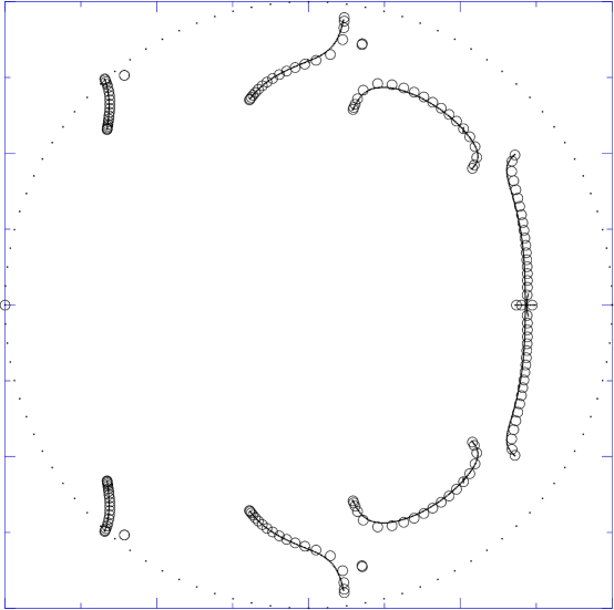
Figure 13: Singular locus ${\cal B}$ for the $L_{x}\to\infty$ limit of the $L_{y}=2$ strip of the $sq_{d}$ lattice with 6-fold multiple transverse edges. For comparison, zeros of the reliability polynomial are shown for this strip with free boundary conditions and $L_{x}=21$. Horizontal and vertical axes are $Re(p)$ and $Im(p)$ with tick spacing 0.25, and the circle $|p-1|=1$ is shown with light dots.

We have also calculated the reliability polynomial for the analogous strip graphs with free longitudinal boundary conditions and with each longitudinal, rather than transverse, edge replaced by 6 edges joining the same pair of vertices. We find similar results. A plot of the zeros for $L_{x}=9$ is shown in Fig. 14. The arcs on ${\cal B}$ that extend outside the disk $|p-1|\leq 1$ are again situated in the upper and lower left, and the endpoints of these arcs that extend outside this disk are

$$p=0.4346475\pm 0.8266808i$$ (5.17.9)

with

$$|p-1|=1.001511$$ (5.17.10)

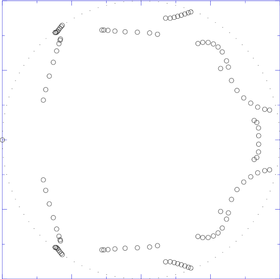
Figure 14: Zeros of the reliability polynomial for the $L_{y}=2,L_{x}=9$ strip of the $sq_{d}$ lattice with 6-fold multiple longitudinal edges and free boundary conditions. Horizontal and vertical axes are $Re(p)$ and $Im(p)$ with tick spacing 0.25, and the circle $|p-1|=1$ is shown with light dots.

5.18 $L_{y}=2$ Free Strip of $K_{4}$ Subgraphs with Multiple Edges

We consider the strip shown in Fig. 8 of the Appendix of [51], but with free, instead of cyclic, longitudinal boundary conditions. In the notation of that figure, we replace each of the edges (labelled as $e_{ij}=(v_{i},v_{j})$) (1,2), (2,3), etc. on the top; (4,5), (5,6), etc. on the bottom, and (1,7), (5,8), (2,9), etc. in the middle with a 6-fold replicated edge. This is a family of planar graphs (as is the family in [51] with cyclic boundary conditions). We calculate the reliability polynomial and find for the numerator and denominator of the generating function

$${\cal N}(p,z)=p\biggl{[}A_{0}+A_{1}z\biggr{]}$$ (5.18.1)

where

$$A_{0}=1$$ (5.18.2)

$$A_{1}=p^{2}(p-1)(p-2)(p^{2}-p+1)(p^{2}-3p+3)(2p^{6}-14p^{5}+42p^{4}-70p^{3}+70p^{2}-42p+13)$$ (5.18.3)

$${\cal D}(p,z)=1+b_{1}z+b_{2}z^{2}$$ (5.18.4)

where

$$b_{1}=p^{2}(6p^{13}-86p^{12}+574p^{11}-2366p^{10}+6734p^{9}-14014p^{8}+22018p^{7}$$ (5.18.5)

(5.18.6)

$$-26561p^{6}+24731p^{5}-17661p^{4}+9471p^{3}-3647p^{2}+918p-118)$$ (5.18.7)

$$b_{2}=p^{4}(1-p)^{3}(4p^{22}-100p^{21}+1201p^{20}-9224p^{19}+50876p^{18}-214544p^{17}$$ (5.18.8)

(5.18.9)

$$+719020p^{16}-1965184p^{15}+4459758p^{14}-8511200p^{13}+13781747p^{12}-19045712p^{11}$$ (5.18.10)

(5.18.11)

$$+22536020p^{10}-22849416p^{9}+19815434p^{8}-14628596p^{7}+9116492p^{6}$$ (5.18.12)

(5.18.13)

$$-4732392p^{5}+2004288p^{4}-670184p^{3}+167360p^{2}-28048p+2401)$$ (5.18.14)

Zeros of the reliability polynomial for the $L_{x}=9$ member of this family are shown in Fig. 15. The tips of two complex-conjugate arcs, again on the upper and lower left, extend outside the disk $|p-1|\leq 1$, ending at the points

$$p=0.4254334\pm 0.8216255i$$ (5.18.15)

which have

$$|p-1|=1.002594$$ (5.18.16)

Thus, as $L_{x}\to\infty$, an infinite number of zeros of the reliability polynomial accumulate to form part of the locus ${\cal B}$ which extends outside the disk $|p-1|\leq 1$. As before, the amount by which some zeros and ${\cal B}$ lie outside the disk is small.

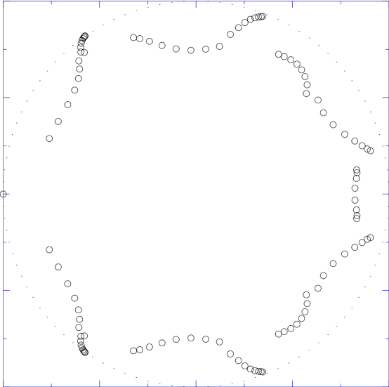
Figure 15: Zeros of the reliability polynomial for the $L_{y}=2,L_{x}=9$ free strip of $K_{4}$ subgraphs with 6-fold multiple longitudinal edges. Horizontal and vertical axes are $Re(p)$ and $Im(p)$ with tick spacing 0.25, and the circle $|p-1|=1$ is shown with light dots.

6 Complete Graphs

The complete graph $K_{n}$ is the graph with $n$ vertices such that every vertex is connected by edges to every other vertex. The family of complete graphs is not a recursive family, and provides a contrast to the recursive families on which we have concentrated in this paper. The reliability polynomial for $K_{n}$ is [6]

$$R(K_{n},p)=1-\sum_{j=1}^{n-1}{n-1\choose j-1}(1-p)^{j(n-j)}R(K_{j},p)\ .$$ (6.1)

Since this family is not recursive, the reliability polynomial does not have the form (4.1.2) and our usual methods for determining an asymptotic accumulation set of zeros as the solution of the degeneracy in magnitudes of dominant $\alpha$ terms do not apply. However, we have studied the zeros of $R(K_{n},p)$ for a wide range of values of $n$, and we find that these zeros typically form an oval-shaped pattern that is concave to the left and is roughly centered around $p=1$, somewhat similar to the exact results that we have established for our recursive families of graphs without multiple edges. As illustrations, we show in Fig. 16 the patterns of zeros for $n=5,10$, and 15. We observe that as $n$ increases, the oval moves outward from $p=1$. Note that since $K_{n}$ is a $\Delta$-regular graph with $\Delta=n-1$, it follows that the vertex degree $\Delta\to\infty$ as $n\to\infty$. This feature that $\Delta\to\infty$ as $n\to\infty$ is thus shared in common by the two families $K_{n}$ and the thick links $TL_{n}$. For the latter family, it is elementary that as $n\to\infty$, ${\cal B}$ is the circle $|p-1|=1$. However, our results show that it is not necessary for any vertex degree to go to infinity in order for a part of ${\cal B}$ to satisfy $|p-1|\geq 1$. Our results for the family of wheel graphs, $G_{D}(1\times m)$ also show that the property that a vertex degree goes to infinity as $|V|\to\infty$ is not sufficient for ${\cal B}$ to have a part with $|p-1|\geq 1$.

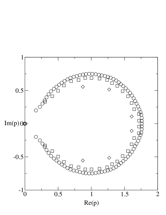
Figure 16: Plot of zeros of the reliability polynomial $R(K_{n},p)$ for $n=$ (a) 5  ($\Diamond$), (b) 10  ($\Box$), (c) 15  ($\circ$).

7 Discussion of Results

In this section we discuss some general features of our results.

• For a given type of lattice and a given width and choice of transverse boundary conditions, we find that in the infinite-length limit, the reliability per vertex $r$ is the same for any choice of longitudinal boundary conditions.

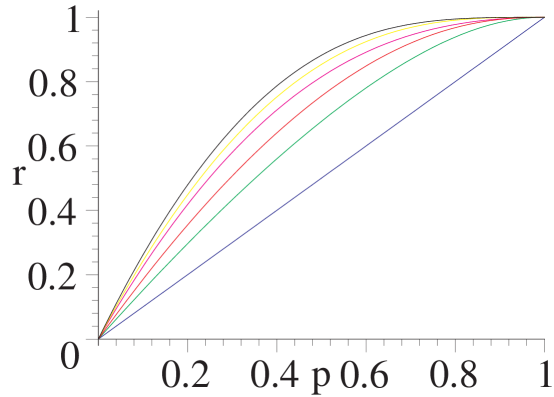
Figure 17: Comparison of asymptotic reliability per vertex $r$ for the $L_{x}\to\infty$ limit of several lattice strips. From bottom to top, the curves refer to (a) $sq[1\times\infty,FBC_{y}]$ with $d_{eff}=2$, (b) $hc[2\times\infty,FBC_{y}]$ with $d_{eff}=2.5$, (c) $sq[2\times\infty,FBC_{y}]$ with $d_{eff}=3$, (d) $sq[2\times\infty,PBC_{y}]$ with $d_{eff}=4$, (e) $G_{D}[1\times\infty]$, same $r$ as for $tri[2\times\infty]$, with $d_{eff}=4$, (f) $G_{D}[2\times\infty]$, with $d_{eff}=4$.

• On general grounds, one expects that the higher the connectivity, and, equivalently for our present purposes, the higher the effective vertex degree $d_{eff}$, the larger the value of $r$ for a fixed $p$. In Fig. 17 we plot $r$ for some strips of the square, triangular, and honeycomb lattices. We see that our expectation is confirmed by our exact results.

• Closely related to this, our results exhibit the property that the derivative $dr/dp$ at $p=0$ is an increasing function of $d_{eff}$. Except for the $L_{y}=1$ strips of the square lattice, i.e., the line and circuit graphs, we find that $dr/dp=0$ at $p=1$ for all strips that we have studied. In Table 3 we list some of the properties that we have found from our calculations.

• We can also comment on features of the zeros of the reliability polynomials and their continuous accumulation sets ${\cal B}$. We find that the zeros of the reliability polynomials for many strips studied do exhibit the property that $|p-1|\leq 1$, as do their loci ${\cal B}$ in the limit of infinite length. However, motivated by [20], we have calculated reliability polynomials for strips such that the zeros of $R(G,p)$ violate the bound $|p-1|\leq 1$ and such that, in the limit of infinite length, the continuous accumulation sets of zeros ${\cal B}$ extend outside of the disk $|p-1|\leq 1$. An intriguing result is that the amounts by which some individual zeros, and the outer part of the loci ${\cal B}$, lie outside this disk are small.

• We find that in some cases, ${\cal B}$ crosses the real axis and hence defines a $p_{c}$, but in other cases, it does not. However, typically, even for families for which ${\cal B}$ does not cross the real axis, there are arc endpoints on ${\cal B}$ that lie close to this axis, thereby enabling one to define a $(p_{c})_{eff}$ via extrapolation or just as the real part of the nearby endpoints. Our results have the property that these values of $p_{c}$ or $(p_{c})_{eff}$ lie in the interval $p\in(1,2]$. It is interesting to discuss the relation between this result and the Brown-Colbourn theorem [16] that $R(G,p)$ does not have any real zeros in the region outside of the set $0\cup(1,2]$. In general, the property that a polynomial has no zeros in an interval of the real axis does not exclude the possibility that as the degree of this polynomial goes to infinity, a resultant continuous accumulation set of zeros ${\cal B}$ crosses the real axis in this interval. A well-known case where this phenomenon does occur is provided by the Potts model partition function. This is a polynomial in $q$ and $a=e^{K}$ with non-negative coefficients. Thus, for fixed positive $q$, for either sign of the spin-spin coupling $J$, this partition function cannot have any zeros on the positive real $a$ axis. However, for the infinite limit of the square lattice, the locus ${\cal B}$ in this case does cross the positive real $a$ axis at the point $a_{c}=1+\sqrt{q}$, which serves as the phase boundary between the paramagnetic and ferromagnetic phases occupying the respective intervals $1\leq a\leq a_{c}$ and $a_{c}\leq a\leq\infty$.

• For all of the lattice strip graphs for which we have calculated $R(G,p)$ and ${\cal B}$, we find that ${\cal B}$ is independent of the longitudinal boundary conditions, although it depends on the transverse boundary conditions and the type of lattice. This requires that the dominant $\alpha$ in the case of cyclic strips must arise from the subset of the $\alpha$’s with coefficient $c^{(0)}$ that coincides with the set of $\alpha$’s for the corresponding strip with free longitudinal boundary conditions. The property that, for a given type of lattice strip, the locus ${\cal B}$ is independent of the longitudinal boundary conditions is quite different from what we found for the corresponding continuous accumulation sets of zeros of chromatic polynomials of lattice strips [31], [43]-[51], which do depend on both longitudinal and transverse boundary conditions.

• For all of the lattice strip graphs for which we have calculated $R(G,p)$ and ${\cal B}$, we find that this locus consists of arcs (and in some cases a line segment) and does not enclose regions in the complex $p$ plane. In some simple cases ${\cal B}$ is connected, but in general, it may consist of several disjoint components. Again, this is quite different from what we found for the loci ${\cal B}$ for chromatic polynomials of lattice strips; for those, a sufficient (not necessary) condition that this locus encloses areas is that the strip has periodic longitudinal boundary conditions [43, 47, 31].

• In all of the cases for which we have calculated exact results, whenever ${\cal B}$ consists of an arc of a circle, then this circle is centered at $p=1$. More generally, even if ${\cal B}$ is not an arc of a circle, it is roughly centered around $p=1$. For families without multiple edges, we find that the component(s) of ${\cal B}$ is (are) roughly concave toward the left.

• The width $L_{y}\to\infty$ limit of loci ${\cal B}$ for the infinite-length lattice strips is not necessarily the same as the continuous accumulation locus of the zeros of the reliability polynomial for the two-dimensional thermodynamic limit $L_{x}\to\infty$, $L_{y}\to\infty$ with $L_{y}/L_{x}$ fixed to a finite nonzero constant. This is clear since for any finite $L_{y}$ regardless of how large, the infinite-length strip is a quasi-one-dimensional system, characterized by the ratio $L_{y}/L_{x}=0$. Thus, for example, the Potts model on these strips has a paramagnetic-ferromagnetic (PM-FM) phase transition point only at $K=\infty$, i.e., $v=\infty$, while for 2D lattices, it has such a PM-FM phase transition point at finite $v$. However, in our previous studies of continuous accumulation sets of loci of Potts model partition functions (e.g., [29]-[38] and our earlier work referred to therein on complex-temperature phase diagrams for Ising models) we have found that it is possible to gain some insight into certain features of the continuous accumulation set of zeros of the Potts model for the two-dimensional thermodynamic limit from studies of wider and wider infinite-length strips.

  In this context, we note that for the (infinite) square lattice, the PM-FM phase transition point for the Potts model is given by $v^{2}=q$ [40]. This transition point is reflected in a nonanalyticity in the free energy of the Potts model at the corresponding temperature variable $v$. As we have discussed and studied in earlier papers, e.g., [53, 54], when one generalizes $v$ to complex values, one sees that a singular point for a real physical value of $v$, such as the PM-FM transition point, is associated with the fact that a complex-temperature phase boundary crosses the real physical $v$ axis at this point. At the crossing points there are physical or complex-temperature singularities in the free energy [53]-[57]. The boundaries on ${\cal B}$ (here as a function of $v$ for fixed $q$, but more generally, also as a function of $q$ for fixed $v$) arise as the continuous accumulation set of the complex-temperature zeros of the partition function, analogous to the origin of the locus ${\cal B}$ studied here as continuous accumulation set of the zeros of the reliability polynomial. Connected with this, the physical paramagnetic, ferromagnetic, and antiferromagnetic (AFM) phases have complex-temperature extensions, and these are separated from each other by the phase boundaries ${\cal B}$ in the $v$ plane. We recall that for the Potts model on the square lattice, the PM and FM phases occupy the intervals $0\leq v\leq\sqrt{q}$ and $\sqrt{q}\leq v\leq\infty$, respectively. Analytically continuing $q$ to real values, using eq. (3.6), we infer that in the limit $q\to 0$ that yields the reliability polynomial, as given by eq. (3.11), the PM phase therefore contracts to a point at $v=0$, which corresponds, via the relation $p=v/(1+v)$ in eq. (3.12), to the point $p=0$, while the FM phase expands to occupy the interval $0\leq v\leq\infty$, corresponding to the interval $0\leq p\leq 1$. As is evident, e.g., in the square-lattice Ising model and more generally for the 2D $q$-state Potts model, the complex-temperature extension of the FM phase includes part of the negative real $v$ axis extending to $v=-\infty$ (as well as the outerlying region $|v|\to\infty$ in the $v$ plane). This semi-infinite interval of large negative real values of $v$ is mapped, via the transformation $p=v/(1+v)$, to a finite interval of values of $p\geq 1$. Points in the outer region $v=Re^{i\theta}$ with $R>>1$ are mapped via this transformation to points in the vicinity of $p=1$, namely $p\simeq 1-R^{-1}e^{-i\theta}$. Since (in the case $q\to 0$ relevant here) all of the points mentioned above in the $v$ plane, namely (i) the interval $0\leq v\leq\infty$, (ii) the interval of large negative real $v$, and (iii) the semi-infinite annular region $v=Re^{i\theta}$ with $R\to\infty$ are in the complex-temperature extension of the FM phase of the Potts model, it follows that the images of these sets of points are all in the same analytically connected region of the $p$ plane as defined by the locus ${\cal B}$. We can draw on another source of information about this boundary as follows. Arguments have been given that for the Potts model on the (infinite) square lattice, the paramagnetic-antiferromagnetic (PM-AFM) transition occurs at a (physical) root of the equation $v(v+4)+q=0$ [59]. Setting $q=0$ and $v=p/(1-p)$ as in (3.11) and (3.12), one finds the solutions $v=0$ and $v=-4$, corresponding respectively to $p=0$, the solution already found above, and $p=4/3$. Hence for the square lattice, the image, under the mapping $v\to p=v/(1+v)$, of the complex-temperature extension of the FM phase includes the real interval $0\leq p\leq 4/3$. The complementary intervals $-\infty\leq p\leq 0$ and $4/3\leq p\leq\infty$ would be part of the image under this map of an unphysical phase denoted the “O” (for “other”) phase in Ref. [53] and our subsequent papers on complex-temperature phase diagrams. Using the fact that the complex-temperature phase boundary separates these various phases, we infer that for the reliability polynomial on the square lattice, in the thermodynamic limit, the zeros accumulate on a locus ${\cal B}$ that is a closed curve crossing the real axis at $p=0$ and $p=4/3$ and separating the interior region from the exterior, which latter includes the intervals $-\infty\leq p\leq 0$ and $4/3\leq p\leq\infty$. In an obvious nomenclature extending that of [53], we denote the regions in the interior and exterior of this closed curve as $R_{FM}$ and $R_{O}$, indicating the correspondence with the complex-temperature phases of the Potts model. Just as the free energy is an analytic function in the interior of a complex-temperature phase, the function $r$ that we have introduced in [15] and here in eq. (1.3) is an analytic function in the regions bounded by the locus ${\cal B}$. One expects qualitatively similar results to hold for the regions of analyticity of $r$ on (the thermodynamic limits of) lattice graphs of dimensionality $d\geq 3$. For the (infinite) square lattice,

  $$p_{c}(sq)=\frac{4}{3}$$ (7.1)

  We shall discuss how this compares with our exact results for $p_{c}$ values on infinite-length finite-width strips below.

  Similar reasoning can be applied to obtain inferences for the loci ${\cal B}$ and the corresponding region diagrams of analyticity of the function $r$ on other (infinite) 2D lattices. For the triangular and honeycomb lattices, the PM-FM phase transition point is given by a (physical) root of the equations $v^{2}(v+3)-q=0$ and $v^{3}-3qv-q^{2}=0$, respectively [61]. Evaluating these for $q=0$ and $v=p/(1-p)$ yields for the triangular lattice, the solutions $p=0$ and $p=3/2$, so that

  $$p_{c}(tri)=\frac{3}{2}$$ (7.2)

  For the honeycomb lattice, the same evaluation yields just the solution $p=0$ and hence does not determine $p_{c}(hc)$ (By the reasoning given above, one can infer that $p_{c}(hc)>1$). The fact that the point $p=0$ on ${\cal B}$ is common to all of the three lattices - square, triangular, and honeycomb - follows because it is the image under the map (3.12) of the point $v=K=0$. This point corresponds to infinite temperature, where, as one can see from eqs. (3.3) and (3.4), the spin-spin interaction does not contribute to $Z(G,q,v)$, which reduces to $q^{|V|}$ for all of these lattices (indeed for any graph $G$).

• For a given type of lattice strip (square, triangular, honeycomb, etc.) and a given set of transverse boundary conditions, we may consider the sequence of loci ${\cal B}$ for each width, $L_{y}$, and inquire whether these approach a limiting locus as $L_{y}\to\infty$. Our results are summarized in Table 3 and are consistent with the hypothesis that such a limiting locus exists. As part of this analysis, we have investigated, for each type of strip family, how $p_{c}$ or $(p_{c})_{eff}$ depends on $L_{y}$. We find that, for a given type of lattice strip and transverse boundary conditions, if a value of $p_{c}$ exists, i.e., if ${\cal B}$ crosses (intersects) the real axis, then $p_{c}$ decreases as $L_{y}$ increases. However, if, for a given type of lattice strip and transverse boundary conditions, one considers the set of values of both $p_{c}$ and $(p_{c})_{eff}$ (the latter for widths where ${\cal B}$ comes close to but does not cross the real axis), then the dependence on $L_{y}$ does not appear to be monotonic. For example, for the infinite-length limit of the strip of the square lattice with free transverse boundary conditions (and any longitudinal boundary conditions), for the width $L_{y}=2$, we have shown that $p_{c}=4/3$. Interestingly, this is the same value as inferred above for the infinite square lattice defined via the usual thermodynamic limit. For the square-lattice strip with width $L_{y}=3$, the locus ${\cal B}$ does not cross the real axis, but, as is evident in Fig. 2, the inner endpoints of the arcs on ${\cal B}$ are sufficiently close to the real axis that one can infer a $(p_{c})_{eff}$, and it is $(p_{c})_{eff}\simeq 1.335$, which is slightly greater than the value of $p_{c}$ for the $L_{y}=2$ strip and the inferred value of $p_{c}(sq)$. As is evident in Table 3, the values of $p_{c}$ are not as close to $p_{c}(sq)$ for the square-lattice strips of the corresponding widths with periodic transverse boundary conditions or self-dual boundary conditions, as compared with free transverse boundary conditions, although they are again consistent with approaching $p_{c}(sq)=4/3$ as the width increases. For the $L_{y}=2$ strip of the triangular lattice, we find the exact result $p_{c}=3/2$. Again, interestingly, this is equal to the inferred value of $p_{c}(tri)$ for the infinite triangular lattice defined via the thermodynamic limit. We have encountered this sort of situation before. For example, for the chromatic polynomial $P(G,q)=Z(G,q,v=-1)$ and its asymptotic limiting function as $|V|\to\infty$, $W(\{G\},q)$ (the degeneracy per vertex for the Potts model), we found that for the infinite-length strip of the triangular lattice with width $L_{y}=3$ and toroidal or Klein-bottle boundary conditions, $q_{c}$ (defined as the maximal point where the continuous accumulation set of zeros of $P(G,q)$ intersects the real $q$ axis) is $q_{c}=4$ [50], the same value as for the infinite triangular lattice. Similarly, for infinite-length limits of self-dual strips of the square lattice, we found $q_{c}=3$ [37, 38], the same value as for the infinite square lattice.

  As regards the behavior of ${\cal B}$ near $p=0$, our results are also consistent with the possibility that for each type of lattice, as the strip width $L_{y}\to\infty$, the respective loci ${\cal B}$ have, on the left, complex-conjugate arc endpoints that come together and join at $p=0$, as motivated by the discussion above for the infinite 2D lattices. The observed feature that this occurs only as a limit, in contrast to the crossing on the right at the respective values of $p_{c}$, can be understood via the relation (3.11) and the aforementioned fact that the infinite-length finite-width strips are quasi-1D systems as far as their thermodynamic behavior is concerned. Since, as we are noted above, the interior of ${\cal B}$ for the reliability polynomial on the 2D lattice corresponds to the image of the complex-temperature extension of the FM phase of the 2D Potts model (for $q\to 0$), and since the argument that this must be separated from other phases relies on the existence of nonzero ferromagnetic long range order (magnetization), it follows that for quasi-1D systems, where for a short-range interaction like that in (3.4), the standard Peierls argument shows that there is no long range order, there is no FM phase. This yields a plausible explanation of the features that we observe in our exact solutions for the infinite-length, finite-width strip graphs, that the loci ${\cal B}$ do not enclose regions in the $p$ plane.

Table 3: Properties of reliability polynomials and resultant loci ${\cal B}$ including $p_{c}$ or $(p_{c})_{eff}$ for various lattice strip graphs. The notation $sqdl$ and $D$ refer to the self-dual strips of the square lattice.

$G_{s}$	$L_{y}$	$BC_{y}$	$BC_{x}$	$d_{eff}$	$N_{\alpha}$	$p_{c}$
sq	1	F	F	2	1	$-$
sq	1	F	P	2	1	$-$
sq	2	F	F	3	2	4/3
sq	2	F	(T)P	3	3	4/3
sq	3	F	F	10/3	4	1.335
sq	3	F	(T)P	10/3	4	1.335
sq	2	P	F	4	2	2
sq	2	P	(T)P	4	3	2
sq	3	P	F	4	3	1.402
sq	3	P	(T)P	4	11	1.402
sq	4	P	F	4	6	1.384
sqdl	1	D	F	4	2	3/2
sqdl	1	D	P	4	3	3/2
sqdl	2	D	F	4	5	1.4
sqdl	2	D	P	4	10	1.4
sqdl	3	D	F	4	14	1.386
sqdl	3	D	P	4	35	1.386
tri	2	F	F	4	2	3/2
tri	2	F	(T)P	4	3	3/2
hc	2	F	F	5/2	2	6/5
hc	2	F	(T)P	5/2	3	6/5

8 Conclusions

In this paper we have presented exact calculations of reliability polynomials $R(G,p)$ for lattice strips $G$ of fixed width and arbitrarily great length with various boundary conditions. We have introduced the notion of a reliability per vertex, $r(\{G\},p)$ and have calculated this exactly for the infinite-length limits of various lattice strip graphs. We have also studied the zeros of $R(G,p)$ in the complex $p$ plane and determine exactly the asymptotic accumulation set of these zeros ${\cal B}$, across which $r(\{G\})$ is nonanalytic. We have observed and discussed several general features of the $r$ functions and the loci ${\cal B}$ for these families of graphs.

Acknowledgment: This research was partially supported by the NSF grant PHY-00-98527.

References

- [1]
- [2] E. F. Moore and C. E. Shannon, Reliable circuits using less reliable components, J. Franklin Inst. 262, 191-208, 281-297 (1956).
- [3] F. Moskowitz, The analysis of redundancy networks, AIEE Trans. Commun. Electronics 39, 627-632 (1958).
- [4] H. Mine, Reliability of physical systems, IRE Trans. Circuit Theory CT-6, 138-151 (1959).
- [5] A. Kel’mans, Connectivity of probabilistic networks, Automation and Remote Control 26, 564-573 (1965).
- [6] C. Colbourn, The Combinatorics of Network Reliability (Oxford Univ. Press, New York, 1987).
- [7] J. Provan and M. Ball, The complexity of counting cuts and of computing the probability that a graph is connected, SIAM J. on Computing, 12, 777-788 (1983).
- [8] M. Lomonosov and V. Polesskii, An upper bound for the reliability of information networks, Problems of Information Transmission 7, 337-339 (1971).
- [9] M. Lomonosov and V. Polesskii, Lower bound of network reliability, Problems of Information Transmission 8, 118-123 (1972).
- [10] J. Kruskal, The number of simplices in a complex, in R. Bellman, ed. Mathematical Optimization Techniques (Univ. California Press, 1963), 251-278.
- [11] R. P. Stanley, The upper bound conjecture and Cohen-Macaulay rings, Studies in Appl. Math. 14, 135-142 (1975).
- [12] M. Ball and J. Provan, Bounds on the reliability polynomial for shellable independence systems, SIAM Journal on Algebraic and Discrete Methods 3, 166-181 (1982).
- [13] M. Ball, C. Colbourn, and J. Provan, “Network reliability”, in Handbook of Operations Research: Network Models (Elsevier North-Holland, 1995), pp. 673-762.
- [14] J. Brown and C. Colbourn, Non-Stanley bounds for network reliability, J. Alg. Combinatorics 5, 18-36 (1996).
- [15] S.-C. Chang and R. Shrock, Tutte polynomials and related asymptotic limiting functions for recursive families of graphs, in Proceedings of the Workshop on Tutte Polynomials, Centre de Recerca Matemàtica, Univ. Autónoma de Barcelona, (Sept. 2001), Advances in Applied. Math., in press (math-ph/0112061).
- [16] J. Brown and C. Colbourn, Roots of the reliability polynomial, SIAM J. Discrete Math. 4, 571-585 (1992).
- [17] D. Wagner, Zeros of reliability polynomials and -vectors of matroids, Combin. Prob., and Computing 9, 167-190 (2000).
- [18] A. Sokal, Bounds on the complex zeros of (di)-chromatic polynomials and Potts-model partition functions, Combin. Prob. Comput. 10, 41-77 (2001). See also [19].
- [19] Y.-B. Choe, J. Oxley, A. Sokal, and D. Wagner, Homogeneous multivariate polynomials with the half-plane property, math.CO/0203034.
- [20] After the submission of the original version of this manuscript (August, 2002), a referee informed us of the Royle-Sokal counterexamples to the Brown-Colbourn conjecture in Nov. 2002. We thank A. Sokal, C. Colbourn, and J. Brown for private communications on this. See G. Royle and A. Sokal, math.CO/0103199.
- [21] W. T. Tutte, A contribution to the theory of chromatic polynomials, Canad. J. Math. 6, 80-91 (1954). Sadly, we must record here that W. T. Tutte died on 2 May, 2002, during the completion of this manuscript.
- [22] W. T. Tutte, On the algebraic theory of graph colourings, J. Combin. Theory 1, 15-50 (1966).
- [23] W. T. Tutte, On dichromatic polynomials, J. Combin. Theory 2, 301-320 (1967).
- [24] W. T. Tutte Graph Theory, vol. 21 of Encyclopedia of Mathematics and its Applications, ed. Rota, G. C. (Addison-Wesley, New York, 1984).
- [25] T. Brylawski and J. Oxley, The Tutte polynomial and its applications, Chap. 6 in Matroid Applications, Encyclopedia of Mathematics and its Applications, vol. 40 (ed. N. White) (Cambridge University Press, Cambridge, 1992), pp. 123-225.
- [26] N. L. Biggs, Algebraic Graph Theory (2nd ed., Cambridge Univ. Press, Cambridge, 1993).
- [27] D. J. A. Welsh, Complexity: Knots, Colourings, and Counting, London Math. Soc. Lect. Note Ser. 186 (Cambridge University Press, Cambridge, 1993).
- [28] B. Bollobás, Modern Graph Theory (Springer, New York, 1998).
- [29] R. Shrock, Exact Potts model partition functions on ladder graphs, Physica A 283, 388-446 (2000).
- [30] S.-C. Chang and R. Shrock, Exact Potts model partition functions on strips of the triangular lattice, Physica A 286, 189-238 (2000).
- [31] R. Shrock, Chromatic polynomials and their zeros and asymptotic limits for families of graphs, in the Proceedings of the 1999 British Combinatorial Conference, BCC99 (July, 1999), Discrete Math. 231, 421-446 (2001).
- [32] S.-C. Chang and R. Shrock, Structural properties of Potts model partition functions and chromatic polynomials for lattice strips, Physica A 296, 131-182 (2001).
- [33] S.-C. Chang and R. Shrock, Exact Potts model partition functions on strips of the honeycomb lattice, Physica A 296, 183-233 (2001).
- [34] S.-C. Chang and R. Shrock, Exact Potts model partition functions on wider arbitrary-length strips of the square lattice, Physica A 296, 234-288 (2001).
- [35] S.-C. Chang and R. Shrock, Exact Partition function for the Potts model with next-nearest neighbor couplings on strips of the square lattice, Int. J. Mod. Phys. B 15, 443-478 (2001).
- [36] S.-C. Chang and R. Shrock, Zeros of Jones polynomials for families of knots and links, Physica A 301, 196-218 (2001).
- [37] S.-C. Chang and R. Shrock, Potts model partition functions for self-dual families of graphs, Physica A 301, 301-329 (2001).
- [38] S.-C. Chang and R. Shrock, Complex-temperature phase diagrams for the -state Potts model on self-dual families of graphs and the nature of the limit, Phys. Rev. E 64, 066116 (2001).
- [39] S.-C. Chang, J. Salas, and R. Shrock, Exact Potts model partition functions for strips of the square lattice, J. Stat. Phys. 107 (2002) 1207-1253.
- [40] F. Y. Wu, The Potts Model, Rev. Mod. Phys. 54, 235-268 (1982).
- [41] F. Y. Wu, Potts model and graph theory, J. Stat. Phys. 52, 99-112 (1988).
- [42] C. Fortuin and P. Kasteleyn, On the random cluster model. I. Introduction and relation to other models, Physica 57, 536-564 (1972).
- [43] R. Shrock and S.-H. Tsai, Asymptotic limits and zeros of chromatic polynomials and ground state entropy of Potts antiferromagnets, Phys. Rev. E 55, 5165-5179 (1997).
- [44] M. Roček, R. Shrock, and S.-H. Tsai, Chromatic polynomials for families of strip graphs and their asymptotic limits, Physica A252, 505-546 (1998).
- [45] R. Shrock and S.-H. Tsai, Ground state entropy of Potts antiferromagnets on homeomorphic families of strip graphs, Physica A259, 315-348 (1998).
- [46] M. Roček, R. Shrock, and S.-H. Tsai, Chromatic polynomials on strip graphs and their asymptotic limits, Physica A259, 367-387 (1998).
- [47] R. Shrock and S.-H. Tsai, Ground state degeneracy of Potts antiferromagnets on 2D lattices: approach using infinite cyclic strip graphs, Phys. Rev. E 60, 3512-3515 (1999).
- [48] R. Shrock and S.-H. Tsai, Exact partition functions for Potts antiferromagnets on cyclic lattice strips, Physica A 275, 429-449 (2000).
- [49] R. Shrock, partition functions for Potts antiferromagnets on Möbius strips and effects of graph topology, Phys. Lett. A261, 57-62 (1999).
- [50] N. L. Biggs and R. Shrock, partition functions for Potts antiferromagnets on square lattice strips with (twisted) periodic boundary conditions, J. Phys. A (Letts) 32, L489-L493 (1999).
- [51] S.-C. Chang and R. Shrock, Ground state entropy of the Potts antiferromagnet with next-nearest-neighbor spin-spin couplings on strips of the square lattice, Phys. Rev. E 62, 4650-4664 (2000).
- [52] R. Shrock and S.-H. Tsai, Ground state entropy of Potts antiferromagnets: bounds, series, and Monte Carlo measurements, Phys. Rev. E 56, 2733-2737 (1997).
- [53] V. Matveev and R. Shrock, Complex-Temperature singularities of the susceptibility in the Ising model: square lattice, J. Phys. A 28 1557-1583 (1995).
- [54] V. Matveev and R. Shrock, Complex-temperature singularities in the Ising model: triangular and honeycomb lattices, J. Phys. A 29, 803-823 (1996).
- [55] V. Matveev and R. Shrock, Complex-Temperature Singularities in Potts Models on the Square Lattice, Phys. Rev. E 54, 6174-6185 (1996).
- [56] H. Feldman, R. Shrock, and S.-H. Tsai, A mapping relating complex and physical temperatures in the 2D -State Potts model and some applications, J. Phys. A (Lett.) 30, L663-668 (1997).
- [57] H. Feldmann, A. J. Guttmann, I. Jensen, R. Shrock, and S.-H. Tsai, Study of the Potts model on the honeycomb and triangular lattices: low-temperature series and partition function zeros, J. Phys. A 31 2287-2310 (1998).
- [58] J. Salas and A. Sokal, Absence of phase transition for antiferromagnetic Potts models via the Dobrushin uniqueness theorem, J. Stat. Phys. 86, 551-579 (1997).
- [59] R. J. Baxter, Critical antiferromagnetic square-lattice Potts model, Proc. Roy. Soc. London, Ser. A 383, 43-54 (1982).
- [60] The results obtained in Ref. [59] involved a mapping from the Potts model to a six-vertex model. A complication pertaining to a mismatch between the boundary conditions for the Potts and vertex model was noted there and in H. Saleur, Zeros of chromatic polynomials: a new approach to Beraha conjecture using quantum groups, Commun. Math. Phys. 132, 657-679 (1990).
- [61] D. Kim and R. Joseph, Exact transition temperature of the Potts model with states per site for the triangular and honeycomb lattices, J. Phys. C 7, L167-L169 (1974).