Small-world properties of the Indian Railway network

Abstract

Structural properties of the Indian Railway network is studied in the light of recent investigations of the scaling properties of different complex networks. Stations are considered as ‘nodes’ and an arbitrary pair of stations is said to be connected by a ‘link’ when at least one train stops at both stations. Rigorous analysis of the existing data shows that the Indian Railway network displays small-world properties. We define and estimate several other quantities associated with this network.

Given a chance, how would we have possibly organized our train travel? People dislike to change trains to reach their destinations. Therefore an extreme possibility would be to run a single train passing through all stations in the country so that no change of train is needed at all! An obvious disadvantage in this strategy is that the average distance between the stations become very large and so also the time needed for travel. The other limiting situation would be, to run a train between any pair of neighbouring stations and try to travel along the minimal paths. This requires a change of train at every station, which is also clearly not economically viable. Railway networks in no country in the world follow either of the two ways, actually they go mid-way. Like any other transport system the main motivation of railways is to be fast and economic. To achieve it, railways run simultaneously many trains, covering short as well as long routes so that a traveller does not need to change more than only a few trains to reach any arbitrary destination in the country.

In this paper we analyse the structure of the Indian Railway network (IRN). This is done in the context of recent investigations of the scaling properties of several complex networks e.g., social, biological, computational networks Small etc. Identifying the stations as nodes of the network and a train which stops at any two stations as the link between the nodes we measure the average distance between an arbitrary pair of stations and find that it depends only logarithmically on the total number of stations in the country. While from the network point of view this implies the small-world nature of the railway network, in practice a traveller has to change only few trains to reach an arbitrary destination. This implies that over years, the railway network has been evolved with the sole aim in mind to make it fast and economic, eventually its structure has become a small-world network WS .

The structure and properties of several social, biological and computational networks like the World-wide web (WWW) web , network of the Internet structure Faloutsos , neural networks neural , collaboration network collab etc. are being studied recently with much interest. In general a network has a number of ‘nodes’ and some ‘links’ connecting different pairs of nodes. Typically the following quantities are defined to characterize a network of $N$ nodes: (i) the diameter is the maximum distance between an arbitrary pair of nodes (ii) the clustering coefficient ${\cal C}(N)$ is the average fraction of connected triplets (iii) the probability distribution $P(k)$ that an arbitrarily selected node has the degree $k$ i.e. this node is linked to $k$ other nodes.

Figure 1: The variation of the mean distance ${\cal D}(N)$ of 25 different subsets of IRN having different number of nodes $(N)$. The whole range is fitted with a function like ${\cal D}(N)=A+B\log(N)$ where $A\approx 1.33$ and $B\approx 0.13$. The inset shows the distribution Prob$(\ell)$ of the shortest path lengths $\ell$ on IRN. The lengths varied to a maximum of only five link lengths and the network has a mean distance ${\cal D}(N)\approx 2.16$.

Watts and Strogatz WS proposed a model of small-world network (SWN) in the context of various social and biological networks. They argued that SWNs must have small diameters which grow as $\ln N$ like random networks but should have large values of the clustering coefficients ${\cal C}(N)\sim 1$ like regular networks. On the other hand the scale-free networks (SFN) are characterized by the power law decay of the degree distribution function: $P(k)\sim k^{-\gamma}$. It was observed later that the degree distributions of nodes for two very important networks e.g., World-wide web web which is a network of web-pages and the hyperlinks among various pages and the Internet network Faloutsos of routers or autonomous systems have scale-free property. Barabási and Albert (BA) proposed a model for SFN which grows from an initial set of nodes and at every time step some additional nodes are introduced which are randomly connected to the previous nodes with the linear attachment probabilities barabasi . All scale-free networks are believed to display small-world properties while a small-world network is not necessarily scale-free.

Figure 2: Variation of the clustering coefficient ${\cal C}(N)$ of 25 different subsets of IRN having different number of nodes $N$. Starting from a somewhat higher value at small number of nodes, the clustering coefficient decreases slowly on increasing $N$ and finally saturates at 0.69.

Networks defined on the Euclidean space have also generated much interests in recent times. Internet, transport systems, postal networks etc. are naturally defined on two-dimensional space. In these generalised networks the attachment probabilities depend jointly on the nodal degrees as well as the lengths of the links euclid1 ; euclid2 .

A railway network is one of the most important examples of transport systems. The very complex topological structures of railway networks have attracted the attention of researchers in many different contexts. For example the fractal nature of the structure of railway networks was studied by Benguigui Benguigui . Very recently the efficiency of Boston subway network has been studied where a new measure for such networks has been proposed boston .

Figure 3: The variation of the clustering coefficient ${\cal C}(k)$ against the degree $k$ for the IRN indicates a logarithmic decay for large $k$.

Our scheme is to associate first a representative graph $G_{N}$ with the IRN of $N$ stations in the following way. Here the stations represent the ‘nodes’ of the graph, whereas two arbitrary stations are considered to be connected by a ‘link’ when there is at least one train which stops at both the stations. These two stations are considered to be at unit distance of separation irrespective of the geographical distance between them. Therefore the shortest distance $\ell_{ij}$ between an arbitrary pair of stations $s_{i}$ and $s_{j}$ is the minimum number of different trains one needs to board on to travel from $s_{i}$ to $s_{j}$. Thus $\ell_{ij}=1$ implies that there is at least one train which stops at both $s_{i}$ and $s_{j}$. Similarly, $\ell_{ij}=2$ implies that there is no train which stops at both $s_{i}$ and $s_{j}$ and one has to change the train at least once in some intermediate station to board the second train to reach $s_{j}$. With this definition, if the trains $t_{1}$, $t_{2}$, $\cdots$ $t_{n}$ pass through a station $s_{i}$, then all the stations through which these $n$ trains pass are unit distance away from $s_{i}$ and are considered as first neighbours of $s_{i}$. Consequently, the number $k_{i}$ of such stations is the degree of the node $s_{i}$.

Indian Railway network is a densely populated network of more than 8000 stations where the number of trains plying in this network is of the order of 10000 IRsite . However, we collected the data of IRN on a coarse-grained level following the recent Indian Railways time table ‘Trains at a Glance’ Timetable containing the important trains and stations in India. This table contains a total of $L=579$ trains covering $N=587$ stations in a total of 86 tables. A grand rectangular matrix ${\cal G}(N,L)$ is then constructed such that the $ij$-th element of this matrix is 1 if the train $j$ stops at the station $i$, otherwise this element is zero. A second matrix ${\cal T}(0:N,N)$ is also constructed where the degree $k_{i}$ of the station $i$ is stored at the element ${\cal T}(0,i)$ and the serial numbers of the $k_{i}$ neighbours of $i$ are stored at the locations ${\cal T}(j,i),j=1,k_{i}$, rest of the elements being zero. We define and estimate the following quantities for the IRN.

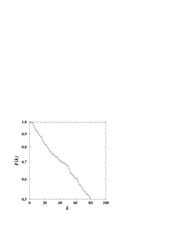
Figure 4: The cumulative degree distribution $F(k)$ of the IRN with the degree $k$ is plotted on the semi-logarithmic scale.

Since $G_{N}$ is a connected graph, there are $N(N-1)/2$ distinct shortest paths among the $N$ stations. We calculate the probability distribution of the shortest path lengths Prob${(\ell)}$. The shortest path lengths are calculated using a burning algorithm Herrmann and using the matrix ${\cal T}$. In this algorithm the fire starts from an arbitrary node $i$, and burns this node at time $t=0$. At time $t=1$ the fire burns all $k_{i}$ neighbours of $i$. At time $t=2$ all unburnt neighbours of $k_{i}$ nodes are burnt and so on. The burning time of a node is the length of the shortest path of that node from the node $i$. This calculation has been repeated for all $N$ nodes to get $N(N-1)/2$ shortest distances. In Fig. 1 inset we plot this distribution which goes to a maximum of $\ell=5$ implying that one needs to change at most four trains to reach any station from any station in India on the coarse-grained level. Similarly the distribution has a peak at $\ell=2$ implying that one can go to the majority of stations in India by changing train only once. In the graph theory the diameter of a graph is measured by the maximum distance between the pairs of nodes. Therefore according to this definition the diameter of our network is exactly equal to 5. However the average shortest path between an arbitrarily selected pair of nodes which we call as the mean distance ${\cal D}(N)$ is also a measure of the topological size of the graph and have been used by many authors to measure the size of networks as described in barabasi . We therefore measure the mean distance ${\cal D}(N)$ of the railway network of $N$ stations as the average shortest distance $\langle{\ell}_{ij}\rangle$ between an arbitrary pair of stations $s_{i}$ and $s_{j}$. We obtain ${\cal D}(N)\approx 2.16$ for this network.

It is desirable to see how ${\cal D}(N)$ varies with $N$ amaral . Since we have the data of a single railway network, we divide the whole IRN into 25 different subsets consisting of trains and stations of 10 different states, 7 different combinations of states, 7 different railway zones and the whole IRN. As a result we obtained 25 data points (though they are not necessarily non-overlapping samples), reflecting the nature of variation of ${\cal D}(N)$ with $N$. In Fig. 1 we plot this data on a semi-log scale and though there is some wild fluctuations for small values of $N$, for large values of $N$ the linear behaviour is quite apparent. The whole range is fitted with ${\cal D}(N)=A+B\log(N)$ where $A\approx 1.33$ and $B\approx 0.13$.

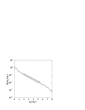
Figure 5: Scaled probability distribution $D_{t}(n_{t})$ for an arbitrary station through which $n_{t}$ trains pass where $\langle n_{t}\rangle\approx 12.06$. Binned data is presented through the circles connected by lines which fits best to an exponential form: $D_{t}(n_{t})\langle n_{t}\rangle=a\exp(-bx)$ with $x=n_{t}/\langle n_{t}\rangle$, $a\approx 0.47$ and $b\approx 0.75$.

The clustering coefficient ${\cal C}(N)$ is defined in the following way. Let the subgraph $G_{i}$ consisting of the neighbours of $s_{i}$ i.e., $(s_{1},s_{2},s_{3},\cdots,s_{k_{i}})$ have $E_{i}$ links among them. Then the clustering co-efficient ${\cal C}_{i}$ of the node $i$ is $2E_{i}/k_{i}(k_{i}-1)$ and that of the whole network is ${\cal C}_{i}=\langle{\cal C}_{i}\rangle$. A direct measure of the clustering co-efficient of the whole IRN gives: ${\cal C}\approx 0.69$ (Fig. 2). The high value of the clustering coefficient is explained in the following way. The number $n_{s}$ of stations in which a particular train stops are all at unit distance from one another on the network and therefore form an $n_{s}$-clique. Therefore if only one train stops at some station $i$ then $C_{i}=1$. When two trains stop at the station $i$ and the sets $n_{s}(1)$ and $n_{s}(2)$ of stations covered by these two trains are different, $C_{i}$ is in general smaller than 1. However there may be other trains which do not stop at $i$ but stop at the stations which are not in both $n_{s}(1)$ and $n_{s}(2)$. These trains enhance the value of $C_{i}$. The value of ${\cal C}\approx 0.69$ is compared with a corresponding random graph network having the same number of vertices and edges as in IRN with the edges distributed randomly. It is found that the number of edges in IRN is 19603. If these edges are distributed randomly within the maximum possible edges on a graph of $N$=587 nodes the the clustering coefficient should be 19603/$[N(N-1)/2]\approx 0.113$ which is the same as Prob(1). We also compute a modified clustering coefficient ${\cal C}_{o}$ by counting in $E_{i}$ only those links in the subgraph $G_{i}$ which pass through the node $i$. We obtained a value ${\cal C}_{o}\approx 0.55$ for the IRN.

Recently, the study of the clustering coefficient as a function of the degree of the node of some real-world network has shown an interesting feature Ravasz ${\cal C}(k)$, defined as the clustering coeffcient of the node with degree $k$, shows a decrease (apparently a power law decay) with $k$ in several networks like the actor, language or world-wide-web networks. However in the network of internet at the router level or power grid network of the Western US, ${\cal C}(k)$ was found to be more or less a constant. In the IRN also, we find that ${\cal C}(k)$ (Fig. 3) remains at a constant value close to unity for small $k$ and shows a logarithmic decay at larger values of $k$. In all these real-world networks where ${\cal C}(k)$ remains more or less a constant, the nodes are linked by physical connections which may be responsible for this common feature. However, in this context it should also be mentioned that the scale-free Barabási-Albert network barabasi also predicts ${\cal C}(k)\propto k^{0}$ and ${\cal C}(N)\propto N^{-0.75}$. In the IRN, although ${\cal C}(N)$ shows a decrease with $N$, it is apparently much slower than a power law.

The degree distribution of the network, that is, the distribution of the number of stations $k$ which are connected by direct trains to an arbitrary station is denoted by $P(k)$. We plot the cumulative degree distribution $F(k)=\int_{k}^{\infty}P(k)dk$ using a semi-log scale in Fig. 4 for the whole IRN. We see that $F(k)$ approximately fits to an exponentially decaying distribution $F(k)\sim exp(-\alpha k)$ with $\alpha$= 0.0085.

Figure 6: Scaled probability distribution $D_{s}(n_{s})$ for an arbitrary train passing through $n_{s}$ stations where $\langle n_{s}\rangle\approx 12.37$. Binned data is presented through the black dots connected by lines which fits best to the form: $D_{s}(n_{s})\langle n_{s}\rangle=ax^{4}/(x^{2}+b)^{3}$ with $x=n_{s}/\langle n_{s}\rangle$, $a\approx 0.6$ and $b\approx 0.096$.

We also calculated the distribution $D(n_{t})$ of the number of trains $n_{t}$ which stop at an arbitrary station. This is plotted in Fig. 5 on a semi-log scale after scaling by the average number of trains $\langle n_{t}\rangle\approx 12.06$ along both the abscissa and the ordinate. The data is binned as before and is fitted to an exponential form: $D_{t}(n_{t})\langle n_{t}\rangle=a\exp(-bx)$ with $x=n_{t}/\langle n_{t}\rangle$, $a\approx 0.47$ and $b\approx 0.75$.

The distribution $D(n_{s})$ of the number of stations through which an arbitrary train passes is plotted in Fig. 6. The data is scaled by the average number of stations $\langle n_{s}\rangle\approx 12.37$ along both the abscissa and the ordinate. The $D(n_{s})$ grows very fast at the beginning, reaches a maximum and then decays to zero. A numerical fit to a functional form like $D_{s}(n_{s})\langle n_{s}\rangle=ax^{4}/(x^{2}+b)^{3}$ with $x=n_{s}/\langle n_{s}\rangle$, $a\approx 0.6$ and $b\approx 0.096$ turns out to be reasonably good.

We also measure the connectivity correlation of IRN following the works of Pastor . Let $F(k^{\prime}|k)$ denote the conditional probability that a node of degree $k$ has a neighbour of degree $k^{\prime}$. Then to see how the nodes of different degrees are correlated we measure the average degree $\langle k_{nn}(k)\rangle=\Sigma_{k^{\prime}}k^{\prime}F(k^{\prime}|k)$ of the subset of nodes which are all neighbours to a particular node of degree $k$. In general this average has a variation like $\langle k_{nn}(k)\rangle\sim k^{-\nu}$ where a non-zero $\nu$ reflects a non-trivial correlation among the nodes of the network. We calculated $\langle k_{nn}(k)\rangle$ for IRN and plotted it in Fig. 7 on a double logarithmic scale. Almost over a decade the $\langle k_{nn}(k)\rangle$ remains same on the average and is independent of $k$, indicating the absence of correlations among the nodes of different degrees.

A more sensitive measure for the degree correlations was proposed in Newman . Newman has defined a degree-degree correlation function $r$ which measures whether a vertex of high degree at one end of a link prefers a vertex of high degree (“assortative mixing”, $r>0$) or low degree (“disassortative mixing” $r<0$) at the other end. It has been observed that social networks are assortative and technological and biological networks are disassortative. We have measured for IRN the normalized correlation function following Newman and found its values to be $r$ = -0.033. This indicates that the IRN is of disassortative nature, i.e. rich vertices at one end of a link show some preference towards poor vertices at the other end, and vice versa.

Figure 7: The variation of the average degree $\langle k_{nn}(k)\rangle$ of the neighbours of a node of degree $k$ with $k$. After some initial fluctuations, $\langle k_{nn}(k)\rangle$ remains almost same over a decade around $k$ = 30 to 300 indicating absence of correlations among the nodes of different degrees.

To summarize, we investigated the structural properties of the Indian Railway network to see if some of the general scaling behaviour obtained for many complex networks in recent times may also be present in IRN. While nodes of the network are evidently the stations, the links are defined as the pairs of stations communicated by single trains. With such a definition of link, the mean distance of the network is a measure of how good is the connectivity of the network. Indeed, we observed that the mean distance of IRN varies logarithmically with the number of nodes with a high value of the clustering coefficient. This implies that IRN behaves like a small-world network, which we believe should be typical of the railway network of any other country, which we are unable to study at present for unavailability of data.

We like to thank I. Bose for constantly encouraging us to work on this problem and also to S. Goswami for suggesting ref. [13]. PS acknowledges financial support from DST grant SP/S2-M11/99. GM acknowledges hospitality in the S. N. Bose National Centre.

References

- (1) D. J. Watts, Small Worlds: The Dynamics of Networks Between Order and Randomness, (Princeton 1999).
- (2) D. J. Watts and S. H. Strogatz, Nature, 393, 440 (1998).
- (3) S. Lawrence and C. L. Giles, Science, 280, 98 (1998); Nature, 400, 107 (1999), R. Albert, H. Jeong and A.-L. Barabási, Nature, 401, 130 (1999).
- (4) M. Faloutsos, P. Faloutsos and C. Faloutsos, Proc. ACM SIGCOMM, Comput. Commun. Rev., 29, 251 (1999).
- (5) J. J. Hopfield and A. V. M. Herz, Proc. Natl. Acad. Sci. USA, 92, 6655 (1995).
- (6) M. E. J. Newman, Proc. Nat. Acad. Sci. USA, 98, 404 (2001); arXiv:cond-mat/0011155.
- (7) A.-L. Barabási and R. Albert, Science, 286, 509 (1999); R. Albert and A.-L. Barabási, Rev. Mod. Phys. 74, 47 (2002).
- (8) S. Jespersen and A. Blumen, Phys. Rev. E 62, 6270 (2000); P. Sen and B. K. Chakrabarti, J. Phys. A 34, 7749 (2001); P. Sen, K. Banerjee and T. Biswas, arXiv:cond-mat/0206570.
- (9) S. S. Manna and P. Sen, arXiv:cond-mat/0203216.
- (10) L. Benguigui and M. Daoud, Geographical Analysis, 23, 362 (1991); H. E. Stanley, Physica A, 186, 1 (1992); L. Benguigui, Environment and Planning A 27, 1147 (1995).
- (11) V. Latora and M. Marchiori, Physica A 314, 109 (2002).
- (12) http://www.indianrail.gov.in/
- (13) A. Kumar, R. K. Thoopal and M. N. Chopra ed. Trains at a Glance, July 2001 - June 2002, Indian Railways, Rail Bhavan, New Delhi.
- (14) H. J. Herrmann, D. C. Hong and H. E. Stanley, J. Phys. A, 17, L261 (1984).
- (15) M. Barthélémy and L. A. N. Amaral, Phys. Rev. Lett. 82, 3180 (1999).
- (16) P. L. Krapivsky and S. Redner, Phys. Rev. E, 63, 066123 (2001); R. Pastor-Satorras, A. Vázquez and A. Vespignani, Phys. Rev. Lett. 87, 258701 (2001).
- (17) E. Ravasz and A.-L. Barabási, arXiv:cond-mat/0206130.
- (18) M. E. J. Newman, arXiv:cond-mat/0205405.