One- and many-body effects on mirages in quantum corrals

Abstract

Recent interesting experiments used scanning tunneling microscopy to study systems involving Kondo impurities in quantum corrals assembled on Cu or noble metal surfaces. The solution of the two-dimensional one-particle Schrödinger equation in a hard wall corral without impurity is useful to predict the conditions under which the Kondo effect can be projected to a remote location (the quantum mirage). To model a soft circular corral, we solve this equation under the potential $W\delta(r-r_{0})$, where $r$ is the distance to the center of the corral and $r_{0}$ its radius. We expand the Green’s function of electron surface states $G_{s}^{0}$ for $r<r_{0}$ as a discrete sum of contributions from single poles at energies $\epsilon_{i}-i\delta_{i}$. The imaginary part $\delta_{i}$ is the half-width of the resonance produced by the soft confining potential, and turns out to be a simple increasing function of $\epsilon_{i}$. In presence of an impurity, we solve the Anderson model at arbitrary temperatures using the resulting expression for $G_{s}^{0}$ and perturbation theory up to second order in the Coulomb repulsion $U$. We calculate the resulting change in the differential conductance $\Delta dI/dV$ as a function of voltage and space, in circular and elliptical corrals, for different conditions, including those corresponding to recent experiments. The main features are reproduced. The role of the direct hybridization between impurity and bulk, the confinement potential, the size of the corral and temperature on the intensity of the mirage are analyzed. We also calculate spin-spin correlation functions.

I Introduction

In recent years, the advances in scanning tunneling microscopy (STM) made possible the manipulation of single atoms on top of a surface and the construction of quantum structures of arbitrary shape eig . In particular, quantum corrals have been assembled by depositing a close line of atoms or molecules on Cu or noble metal (111) surfaces cro ; hel ; man ; man2 . These surfaces have the property that for small wave vectors parallel to the surface a parabolic band of two-dimensional (2D) surface states uncoupled to bulk states exists hub . A circular corral of radius $71.3$ Å was constructed depositing 48 Fe atoms on a Cu(111) surface cro . The measured differential conductance $dI/dV$ could be fitted by a combination of the density of eigenstates close to the Fermi energy $\epsilon_{F}$, of a 2D electron gas inside a hard wall circular corral cro . On another experiment, a Co atom acting as a magnetic impurity was placed at one focus of an elliptical quantum corral, and the corresponding Kondo feature in $dI/dV$ was observed not only at that position, but also with reduced intensity at the other focus man . This “mirage” can be understood as the result of quantum interference in the way in which the Kondo effect is transmitted from one focus to the other by the different conduction eigenstates of a hard-wall ellipse rap . Among these eigenstates, the density of the one closest to $\epsilon_{F}$ is clearly displayed in the change of differential conductance $\Delta dI/dV$ after adding the impurity man . More recently, the extrema in the degenerate $37^{th}$ and $38^{th}$ conduction eigenstates of a hard wall circular corral have inspired an experiment with two impurities inside the corral man2 .

The theories of the mirage experiment can be classified into those which start from eigenstates of a confined 2D electron gas rap ; por ; wei ; hal ; ali2 ; wil and those in which the confining atoms are modeled by a phenomenological scattering approach aga ; fie . The latter have the disadvantage that many-body effects are very hard to include. In addition, some features which are clear from the hard wall eigenstates, like mirages out of the foci man2 ; rap ; por ; wei , are somewhat hidden in the scattering approaches. On the other hand, while the eigenstates inside a hard wall corral are perfectly defined, in the actual experiments the boundaries of the corrals are soft and the eigenstates become resonances with finite width $\delta_{i}$ cro . This width plays a crucial role in the line shape of $\Delta dI/dV$ and its magnitude at the mirage point rap ; ali2 . If $\delta_{i}$ is large the mirage disappears, while if $\delta_{i}=0$ and other parameters as in the experiment, there is no Kondo resonance at $\epsilon_{F}$. Ordinary Lanczos calculations have $\delta_{i}=0$ hal and are unable to describe the line shape of $\Delta dI/dV$. This can be corrected using an embedding method wil . To the best of our knowledge, this theory and the perturbative one rap ; ali2 using a constant value for $\delta_{i}=\delta$ as a parameter, are the only many-body ones presented so far, which can explain the voltage dependence of $\Delta dI/dV$. Thus, a careful study of the broadening $\delta_{i}$ is necessary.

Another important parameter which is still not well known is $\delta_{b}/\delta_{s}$, where $\delta_{b}$ ($\delta_{s}$) is the part of the resonant level width of the impurity state, which is due to hybridization with bulk (surface) states. Some theories have assumed that $\delta_{b}\sim\delta_{s}$, while others have taken $\delta_{b}=0$ rap ; por ; wei ; hal ; ali2 . Clearly, $\delta_{s}\neq 0$, because otherwise $\Delta dI/dV$ would be independent of the 2D conduction eigenstates in contrast to the experiment man . Instead, the line shape for both, the elliptical corral and the clean surface can be explained taking $\delta_{s}=0$ and the same set of parameters ali2 . A recent experiment suggests that $\delta_{b}>\delta_{s}$ on the basis of the rapid decay in $\Delta dI/dV$ as the STM tip is moved away from the impurity knorr . However, the 4s and 4p states of the impurity atom were not included in the analysis and they can affect the distance dependence of $\Delta dI/dV$. Recently, it has been suggested that experiments with two impurities inside a quantum corral can elucidate the magnitude of $\delta_{b}/\delta_{s}$ because the effect of interactions between impurities is expected to be proportional to $\delta_{s}^{2}$wil .

In this work we solve the impurity Anderson model which describes the mirage experiment using perturbation theory in the Coulomb repulsion $U$. The previous theory of one of us rap is extended to include non-vanishing $\delta_{b}$ and a more realistic $\delta_{i}$. We calculate the widths of the conduction states $\delta_{i}$ for a circular corral. We obtain an integral expression for the conduction electron Green’s function $G_{s}^{0}$ in the absence of the impurity, and then we expand it as a discrete sum of contributions from simple poles, using ideas borrowed from nuclear physics cal and scattering theory tay . This expansion takes a suitable form for the perturbative approach. We also discuss the space dependence of the compensation of the impurity spin. The calculation of $G_{s}^{0}$ is presented in section II. In section III we describe the model and the many-body approach. Section IV contains the results for $\Delta dI/dV$ in circular and elliptical corrals with a magnetic impurity. In Section V, we calculate the correlation functions between the impurity spin and that of the conduction electrons as a function of position. Section VI is a discussion.

II The clean circular corral

Starting from free electrons in 2D, we model the boundary of an empty circular corral (without magnetic impurities inside) by a continuous potential $W\delta(r-r_{0})$, where $r$ is the distance to the center of the circle and $r_{0}$ its radius. The approximation of a continuous boundary (instead of discrete adatoms forming the corral) simplifies considerably the mathematics and is justified by the fact that the Fermi wave length for surface electrons $2\pi/k_{F}\simeq 30$ Å is larger than the average distance between adatoms $\sim 10$ Å. The angular momentum projection perpendicular to the surface $l_{z}=m$ becomes a good quantum number, due to the rotational symmetry around the center of the corral. For each $m$ and energy $E=(\hbar k)^{2}/(2m_{e}^{*})$, where $m_{e}^{*}$ is the effective mass, the eigenstates can be written in the form $\varphi_{km}(r,\theta)=\psi_{km}(kr)\ e^{im\theta}$ in polar coordinates, and the 2D radial Schrödinger equation becomes

$$-\frac{\hbar^{2}}{2m_{e}^{*}}\frac{1}{r}\frac{\partial\ }{\partial r}\left(r\frac{\partial\psi_{km}}{\partial r}\right)+[\frac{\ (\hbar m)^{2}}{2m_{e}^{*}r^{2}}+W\delta(r-r_{0})-E]\psi_{km}=0.$$ (1)

Its solution can be written in the form $\psi_{km}=\psi_{km}^{<}\theta(r_{0}-r)+\psi_{km}^{>}\theta(r-r_{0})$, where $\theta(r)$ is the step function and (except for a normalization constant):

$$\psi_{k,m}^{<} = J_{m}(kr)$$

$$\psi_{k,m}^{>} = A_{m}(k)J_{m}(kr)+B_{m}(k)Y_{m}(kr),$$ (2)

where $J_{m}(Y_{m})$ is the Bessel function of the first (second) kind. From the continuity of $\psi_{km}$ and the discontinuity in the first derivative according to Eq. (1), and using known expressions for the derivatives of the Bessel functions abra , one obtains:

$$A_{m}(k) = 1+\frac{2m_{e}^{*}W/(\hbar^{2}k)}{\frac{Y_{m+1}(kr_{0})}{Y_{m}(kr_{0})}-\frac{J_{m+1}(kr_{0})}{J_{m}(kr_{0})}},$$

$$B_{m}(k) = \left(1-A_{m}(k)\right)\frac{J_{m}(kr_{0})}{Y_{m}(kr_{0})}.$$ (3)

We normalize the wave functions $\varphi_{km}(r,\theta)$ inside a hard wall box of large radius $R$ and take the limit $R\rightarrow+\infty$. A quantity of interest in the many-body problem (see Eq. (15)) is the Green’s function for surface conduction electrons in the absence of the impurity:

$$G_{s}^{0}(z;r,\theta,r^{\prime},\theta^{\prime})=\sum_{km}\frac{\varphi_{km}(r,\theta)\overline{\varphi}_{km}(r^{\prime},\theta^{\prime})}{z-\epsilon_{km}},$$ (4)

where the bar over $\varphi_{km}$ denotes complex conjugation and the sum over $k$ extends over all radial wave vectors for which $\varphi_{km}(R,\theta)=0$. Using Eqs. (2) and (3), and taking the limit $R\rightarrow+\infty$, we obtain after some algebra for $r,r^{\prime}<r_{0}$

$$G_{s}^{0}(z;r,\theta,r^{\prime},\theta^{\prime})=\sum_{m}\int\frac{dk\ k\ J_{m}(kr)J_{m}(kr^{\prime})\ e^{im(\theta-\theta^{\prime})}}{2\pi\left(A_{m}^{2}(k)+B_{m}^{2}(k)\right)\left(z-\frac{(\hbar k)^{2}}{2m_{e}^{*}}\right)}.$$ (5)

When $W\rightarrow+\infty$, it is easy to see that $A_{m},B_{m}\rightarrow\infty$, except for those values of $k$ for which $J_{l}(kr_{0})=0$, and one recovers the known result for the hard wall problem

$$G_{s}^{0}=\sum_{n,m}\frac{J_{m}(\gamma_{n}^{m}r)J_{m}(\gamma_{n}^{m}r^{\prime})\ e^{im(\theta-\theta^{\prime})}}{\left(\sqrt{\pi}r_{0}J_{m+1}(\gamma_{n}^{m}r_{0})\right)^{2}\left(z-\frac{(\hbar\gamma_{n}^{m})^{2}}{2m_{e}^{*}}\right)},$$ (6)

where $\gamma_{n}^{m}r_{0}$ is the $n^{th}$ zero of $J_{m}(\alpha)$. For finite $W$ one expects that the poles of Eq. (6) become resonances described by appropriate complex poles of the scattering matrix cal ; tay . Actually, the integral of Eq. (5) can be thought as an integral over energy $E(k)=(\hbar k)^{2}/(2m_{e}^{*})$ and for any $z$ in the upper half of the complex plane, the integrand is analytical in $E$, except at the zeros of $A_{m}^{2}+B_{m}^{2}$. The physical zeros of $A_{m}^{2}+B_{m}^{2}$ lie in the lower half plane of $E$. Then in principle one can evaluate the integral by the method of residues. A technical problem is that the Bessel functions diverge for infinite complex $k$ and one has to assume a high energy cut off. This however has no physical consequences. Thus, $G_{s}^{0}$ can be written in the form:

$$G_{s}^{0}=\sum_{n,m}\frac{C_{n}^{m}\ J_{m}(k_{n}^{m}r)J_{m}(k_{n}^{m}r^{\prime})\ e^{im(\theta-\theta^{\prime})}}{z-\epsilon_{n}^{m}+i\delta_{n}^{m}},$$ (7)

where $k_{n}^{m}$ are the complex zeros of $A_{m}^{2}(k)+B_{m}^{2}(k)$, with $(\hbar k_{n}^{m})^{2}/(2m_{e}^{*})=\epsilon_{n}^{m}-i\delta_{n}^{m}$, $\delta_{n}^{m}>0$, and from the residues of the integrand in Eq. (5) one obtains:

$$C_{n}^{m}=-\frac{i\ k_{n}^{m}}{\frac{\partial(A_{m}^{2}(k)+B_{m}^{2}(k))}{\partial k}|_{k=k_{n}^{m}}}.$$ (8)

In practice, in Eq.(7) we include only the terms for which $\epsilon_{n}^{m}<E_{c}$, where the cut off energy $E_{c}$ is typically taken as three times the Fermi energy. Thus, Eq. (7) is an asymptotic low-energy expansion. It reduces to Eq. (6) for a hard-wall corral.

A quantity of interest (because it is proportional to $dI/dV$ knorr ; schi ) is the local density of conduction states $\rho_{s}^{0}(r,\theta,\epsilon)$ which for $r<r_{0}$ is given by

$$\rho_{s}^{0}(r,\theta,\epsilon)=\lim_{\eta\rightarrow 0^{+}}\ -\frac{1}{\pi}\mathop{\rm Im}G_{s}^{0}(\epsilon+i\eta;r,\theta,r,\theta).$$ (9)

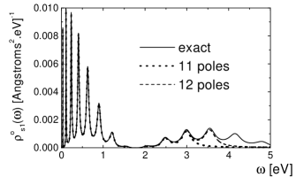
Figure 1: Partial contribution of conduction states with $m=1$ to the local density of states, and approximation using a summation of a finite number of contributions from poles in Eqs. (7), (8), as a function of energy for $W=15\hbar^{2}/(2m_{e}^{*}r_{0})$ and $r=0.14\ r_{0}$.

In Fig. 1 we compare the contribution to the exact $\rho_{s}^{0}$ of the states with angular momentum projection $m=1$, with the corresponding expression using the partial summation in Eq. (7). We have taken an effective mass $m_{e}^{*}=0.38\ m_{e}$ where $m_{e}$ is the electron mass cro ; euc . As in recent experiments man2 , we have taken $r_{0}=63.5$ Å, so that the fourth state (ordered in increasing energy) with $m=1$ falls at $\epsilon_{F}$ note . Finally we took $W=15\hbar^{2}/(2m_{e}^{*}r_{0})\simeq 2.37\$eVÅ in order that the width of this state would be $\delta_{4}^{1}=0.0213$ eV, similar to that reported in some experiments cro . The point of observation $r=0.14r_{0}$ was taken at the maximum of $J_{1}(\gamma_{4}^{1}r)$. One can see that the result in Fig 1 is consistent with the fact expected from previous studies with potentials that vanish except in a finite region cal : the discrete sum Eq. (7) reproduces the low-energy part of $G_{s}^{0}$.

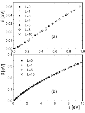
Figure 2: Width of the energy levels as a function of energy, for (a) $0<\epsilon_{n}^{m}<1$ eV and (b) $0<\epsilon_{n}^{m}<10$ eV.

In Fig. 2 we represent $\delta_{n}^{m}$ as a function of $\epsilon_{n}^{m}$. As a first approximation, $\delta_{n}^{m}/\epsilon_{n}^{m}$ is a constant, independent of $m$ and $n$. In any case, $\delta_{n}^{m}$ seems to depend on $n$ and $m$ only through $\epsilon_{n}^{m}$. This result is surprising. For a given confining potential $W$, one would naively expect that $\delta_{n}^{m}$ increases with the radial part of the kinetic energy, being rather independent of the angular part. However, as $m$ increases, the weight of the wave functions near the border of the corral ($r\sim r_{0}$) also increases and compensates the decay in radial velocity.

To study the effects of changes in the magnitude of the confining potential, we started form a situation with $\epsilon_{4}^{1}=\epsilon_{F}$ for rigid walls ($W\rightarrow+\infty$). As $W$ decreases, $\epsilon_{4}^{1}$ decreases slightly, its width $\delta_{4}^{1}$ increases and the position $r_{M}$ of the maximum of $\rho_{s}^{0}(r,\theta,\epsilon)$ for $\epsilon=\epsilon_{4}^{1}$ deviates from its value $0.138r_{0}$ for $W\rightarrow+\infty$ towards larger values. These changes are illustrated in Table 1. The change in $\epsilon_{4}^{1}$ can be interpreted, in a first approximation, as a small increase of the effective mass. In fact, using known properties of the Bessel functions abra , it can be shown that for $W\rightarrow\infty$, the effective mass increases by a factor $1+\hbar^{2}/(m^{*}_{e}r_{0}W)$. Fitting the lowest energies of a circular corral with a model with hard walls, gives $m_{e}^{*}=0.38\ m_{e}$ cro ; note . For moderate $W$, it seems that $\delta^{1}_{4}\sim 1/W$, however for large $W$, $\delta^{m}_{n}\sim 1/W^{2}$ . In contrast to $\delta_{4}^{1}$, $r_{m}$ is only weakly dependent on $W$ (see Table 1).

$W\ \left[\frac{\hbar{{}^{2}}}{2m^{*}r_{0}}\right]$	$\delta_{4}^{1}\ [meV]$	$\epsilon_{4}^{1}\ [meV]$	Maximum[% $r_{o}$]
0.1	171.4	364.8	14.81
1	100.2	381.3	14.74
5	51.0	393.1	14.60
7	41.2	396.1	14.55
10	31.3	400.7	14.48
12	26.6	403.1	14.44
15	21.3	406.4	14.39
18	17.4	409.3	14.34
$\infty$	0	441.1	13.80

Table 1: Variation of the energy $\epsilon_{4}^{1}$, its width $\delta_{4}^{1}$ and the position of the maximum of $\rho(r,\theta,\epsilon_{4}^{1})$ as a function of the confining potential $W$.

What happens with $\epsilon_{n}^{m}$ and $\delta_{n}^{m}$ if the size of the corral is changed? We expect that $W$ remains constant, independent of $r_{0}$. If $r_{0}$ is increased by a factor $f$, changing variables in the Schrödinger equation (1), to $\rho=r/f$, one realizes that (except for normalization) the following equality holds for the wave functions of given projection, position, energy and parameters of the potential:

$$\varphi_{m}(r,\theta,\epsilon,fr_{0},W)\equiv\varphi_{m}(\frac{r}{f},\theta,f^{2}\epsilon,r_{0},fW).$$ (10)

Then, increasing $r_{0}$ by a factor $f$ one expects, as a first approximation, a radial dilation by a factor $f$ of the corresponding wave function, a compression of the energy levels $\epsilon$ by a factor of $f^{2}$, and for large $W$, that the widths $\delta_{i}$ remain approximately constant.

III The many-body problem

In this section, we explain the model and approximations used to describe the electronic structure of a system composed of a quantum corral and a magnetic impurity inside it. Basically we consider surface states, described inside the corral by a Green function $G_{s}^{0}$ like that discussed in the previous section, hybridized with one localized $d$ orbital with an important on-site repulsion $U$ rap ; por ; hal ; ali2 . We also include an hybridization of the $d$ orbital with bulk states. We are neglecting the degeneracy of the $d$ level, which we believe is not important for the essential physics, and other $s,p$ orbitals brought by the impurity which might affect the magnitude of $dI/dV$ near the site impurity.

The Hamiltonian can be written as:

$$H = \sum_{j\sigma}\varepsilon_{j}s_{j\sigma}^{\dagger}s_{j\sigma}+\sum_{j\sigma}\varepsilon_{j}^{b}b_{j\sigma}^{\dagger}b_{j\sigma}+E_{d}\sum_{i\sigma}d_{i\sigma}^{\dagger}d_{i\sigma}+$$ (11)

$$+U\sum d_{\uparrow}^{\dagger}d_{\uparrow}d_{\downarrow}^{\dagger}d_{\downarrow}+\sum_{j\sigma}V_{s}\lambda[\varphi_{j}(R_{i})d_{\sigma}^{\dagger}s_{j\sigma}+\text{H.c.}]+$$

$$+\sum_{j\sigma}V_{b}^{j}[d_{\sigma}^{\dagger}b_{j\sigma}+\text{H.c.}].$$

where $s_{j\sigma}^{\dagger}$ ($b_{j\sigma}^{\dagger}$) are creation operators for an electron in the $j^{th}$ surface (bulk) conduction eigenstate in the absence of the impurity but including the corral. The impurity is placed at the two-dimensional position $R_{i}$ on the surface, and we assume that the hybridization of the impurity $d$ orbital with the surface state $j$ is proportional to its normalized wave function at that point $\varphi_{j}(R_{i})$. We write the proportionality constant as $V_{s}\lambda$, where $V_{s}$ is an energy (representing the hybridization in a tight binding model wei ; ali2 ) and $\lambda=2.38$ Å is the square root of the surface per Cu atom of a Cu(111) surface.

At sufficiently low temperature, the differential conductance $dI/dV$ when the STM tip is at position $R_{t}$ is proportional to the density of the mixed state schi ,

$$f_{\sigma}(R_{t})=\lambda\sum_{j}\varphi_{j}(R_{t})s_{j\sigma}+qd_{\sigma},$$ (12)

$$\frac{dI(V)}{dV}\sim\rho_{f}(\epsilon_{F}+eV)=-\frac{1}{\pi}\mathop{\rm Im}G_{f}^{\sigma}(\epsilon_{F}+eV),$$ (13)

where $G_{f}^{\sigma}(\omega)=\langle\langle f_{\sigma};f_{\sigma}^{\dagger}\rangle\rangle_{\omega}$ is the Green function of $f_{\sigma}(R_{t})$, and $q(R_{t})$ is the ratio between the tunneling matrix elements tip-impurity and tip-surface, and is significant only for very small $R_{t}-R_{i}$, due to the rapid decay of the wave functions for $d$ states.

Using the equations of motion

$$(\omega-\epsilon_{j})\langle\langle s_{j\sigma};s_{j\prime\sigma}^{\dagger}\rangle\rangle_{\omega} = \delta_{jj\prime}+V_{s}\lambda\overline{\varphi}_{j}(R_{i})\langle\langle d_{\sigma};s_{j\prime,\sigma}^{\dagger}\rangle\rangle_{\omega},$$

$$(\omega-\epsilon_{j})\langle\langle s_{j\sigma};d_{\sigma}^{\dagger}\rangle\rangle_{\omega} = V_{s}\lambda\overline{\varphi}_{j}(R_{i})\langle\langle d_{\sigma};d_{\sigma}^{\dagger}\rangle\rangle_{\omega},$$

$$(\omega-\epsilon_{j\prime})\langle\langle d_{\sigma};s_{j\prime\sigma}^{\dagger}\rangle\rangle_{\omega} = V_{s}\lambda\varphi_{j\prime}(R_{i})\langle\langle d_{\sigma};d_{\sigma}^{\dagger}\rangle\rangle_{\omega},$$ (14)

$G_{f}^{\sigma}$ is expressed in terms of the Green function for the $d$ electrons $G_{d}^{\sigma}(\omega)=\langle\langle d_{\sigma};d_{\sigma}^{\dagger}\rangle\rangle_{\omega}$, and the unperturbed conduction electron Green function for surface states $G_{s}^{0}$ . We drop the superscript $\sigma$ in the following because of the spin independence of the problem. The difference in $G_{f}$ between the results with and without impurity becomes:

$$\Delta G_{f}=\left(V_{s}\lambda^{2}G_{s}^{0}(R_{t},R_{i},\omega)+q\right)\times$$

$$\times\left(V_{s}\lambda^{2}G_{s}^{0}(R_{i},R_{t},\omega)+q\right)G_{d},.$$ (15)

where

$$G_{s}^{0}(R_{1},R_{2},\omega)=\sum_{j}\frac{\varphi_{j}(R_{1})\overline{\varphi}_{j}(R_{2})}{\omega-\epsilon_{j}}.$$ (16)

We assume that $G_{s}^{0}$ is known from the one-body problem. For the circular corral, it has been discussed in the previous section.

The remaining task is to calculate $G_{d}$ using a many-body approach. The most accurate calculation would be to use the Wilson renormalization group wrg . However, the particular structure of the one-body problem, and the lack of continuous symmetries in the general case renders its application very difficult. We have used perturbation theory up to second order in $U$ yos ; hor . Near the symmetric case $E_{d}+U/2=\epsilon_{F}$, the theory is quantitatively correct up to $U\sim 8\Delta$, where $\Delta$ is the resonant level width sil . Out of the symmetric case, interpolative self-consistent schemes lev ; kaj still work for moderately large values of $U$ dots ; pc . In particular, the persistent current in small rings with quantum dots practically coincides with exact results pc . Here we assume a situation in which the effective one-particle $d$ level $E_{d}^{eff}=E_{d}+U\langle d_{\sigma}^{\dagger}d_{\sigma}\rangle$ is very near the Fermi level. This is justified by first-principle calculations llois and allows us to avoid selfconsistency.

Then:

$$[G_{d}(\omega)]^{-1}=[G_{d}^{0}(\omega)]^{-1}-\Sigma(\omega),$$ (17)

where $G_{d}^{0}$ is $G_{d}$ for $U=0$ and $E_{d}$ replaced by $E_{d}^{eff}$, and $\Sigma(\omega)$ is the self-energy up to second order in $U$ evaluated from a Feynmann diagram involving the analytical extension of the time ordered $G_{d}^{0}$ to Matsubara frequencies yos ; hor :

$$\Sigma(i\omega_{l},T) = U^{2}T\sum_{m}G_{d}^{0}(i\omega_{l}-i\nu_{m})\chi(i\nu_{m}),$$ (18)

$$\chi(i\nu_{m}) = -T\sum_{n}G_{d}^{0}(i\omega_{n})G_{d}^{0}(i\omega_{n}+i\nu_{m}),$$ (19)

where $\omega_{n}=(2n+1)\pi T$ and $\nu_{m}=2n\pi T$.

From the equation of motion of $G_{d}$ for $U=0$ and using Eqs. (14) we obtain

$$G_{d}^{0}(\omega)=\frac{1}{\omega-E_{d}^{eff}+i\delta_{b}-(V\lambda)^{2}G_{s}^{0}(R_{i},R_{i},\omega)},$$ (20)

where we have replaced

$$\text{Im}\sum_{i}\frac{|V_{b}^{i}|^{2}}{\omega+i\eta-\epsilon_{i}}=-\delta_{b}$$ (21)

assuming that the $V_{b}^{i}$ and the bulk density of states are featureless near $\epsilon_{F}$ and can be replaced by a constant. The real part of the sum can be absorbed in $E_{d}^{eff}$.

From the discussion of section II, and previous works cal , we know that $G_{s}^{0}(R_{i},R_{i},\omega)$ can be expanded as a sum of contributions from discrete poles. In particular, for the circular corral, $G_{s}^{0}(\omega;r,\theta,r^{\prime},\theta^{\prime})$ is given by Eqs. (7) and (8). For other shapes of the corral, the results of the previous section suggest that within errors of a few percent:

$$G_{s}^{0}(\omega,R_{1},R_{2})\simeq\sum_{j}\frac{\varphi_{j}^{c}(R_{1})\overline{\varphi}_{j}^{c}(R_{2})}{\omega-\epsilon_{j}+i\delta_{F}\epsilon_{j}/\epsilon_{F}},$$ (22)

where now $\varphi_{j}^{c}(R)$ are the discrete eigenstates of the hard wall corral and $\epsilon_{j}$ are their energies, calculated with a slightly renormalized mass. $\delta_{F}$ is the width of the resonance at the Fermi level. In practice we cut off the sum in Eq. (22) at an energy $\sim 3\epsilon_{F}$, retaining $N$ poles. Then, $G_{d}^{0}(\omega)$ can be expressed as a sum of $N+1$ poles and residues at these poles notepol Denoting the poles of $G_{d}^{0}(\omega)$ by $r_{l}-i\delta_{l}$ and their residues by $a_{l}$, we can write:

$$G_{d}^{0}(\omega)=\sum_{l=1}^{N+1}\frac{a_{l}}{\omega-r_{l}+i\delta_{l}}.$$ (23)

This is the retarded Green function. In order to evaluate perturbative diagrams, like Eqs. (18), (19), one needs the analytical extension of the time ordered Green function to imaginary frequencies $\omega\rightarrow i\omega_{n}$ mahan ; note2 :

$$G_{d}^{0}(i\omega_{n})=\sum_{l}\frac{a_{l}+\overline{a_{l}}+(a_{l}-\overline{a_{l}})\text{sgn}(\omega_{n})}{2\left[i\omega_{n}+i\delta_{l}\text{sgn}(\omega_{n})-r_{l}\right]},$$ (24)

where $\overline{a_{l}}$ is the complex conjugate of $a_{l}$ and sgn$(x)$ is the sign of $x$. Here and in what follows, the origin of energies has been placed at the Fermi energy $(\epsilon_{F}=0)$ for simplicity.

Using standard methods mahan , the sums over Matsubara frequencies, Eqs. (18), (19) can be transformed into integrals over branch cuts. The first integral can be done analytically in terms of the digamma function $\Psi(z)$ abra . A lengthy but straightforward algebra after analytical continuation back to real $\omega$ leads to:

$$\Sigma(\omega) = \frac{U^{2}}{\pi}\int_{-\infty}^{\infty}dy\ [\frac{1}{e^{y/T}-1}G_{d}^{0}(\omega-y)\mathop{\rm Im}\chi(y)+$$ (25)

$$+\frac{1}{e^{y/T}+1}\text{Im}G_{d}^{0}(-y)\ \chi(\omega+y)],$$

where

$$\chi(\omega) = -\frac{i}{2\pi}\ \sum_{lm}\left(A_{lm}(\omega)-B_{lm}(\omega)\right)\Psi_{l}(0)+$$ (26)

$$+\left(\overline{B_{lm}}(-\omega)-\overline{A_{lm}}(-\omega)\right)\overline{\Psi_{l}}(0)+$$

$$-\left(B_{lm}(\omega)+A_{lm}(-\omega)\right)\Psi_{l}(\omega)-$$

$$-\left(\overline{B_{lm}}(-\omega)+\overline{A_{lm}}(\omega)\right)\overline{\Psi_{l}}(-\omega),$$

with

$$A_{lm}(\omega) = \frac{a_{l}\ a_{m}}{\omega+r_{l}-r_{m}-i\delta_{l}+i\delta_{m}},$$

$$B_{lm}(\omega) = \frac{a_{l}\ \overline{a_{m}}}{\omega-r_{l}+r_{m}+i\delta_{l}+i\delta_{m}},$$

$$\Psi_{l}(\omega) = \Psi\left(\frac{1}{2}+\frac{\delta_{l}+i(r_{l}-\omega)}{2\pi T}\right).$$ (27)

Summarizing, our approximation for the Green function of the $d$ electrons $G_{d}$ consist in the following steps: we first decompose the unperturbed Green function $G_{d}^{0}$ given by Eq. (20), and (7) or (22) into a sum of poles, Eq. (23). Then, the self-energy $\Sigma(\omega)$ is calculated using Eqs. (25), (26) and (27), and finally $G_{d}$ is obtained from Eq. (17). The change in $dI/dV$ after adding the impurity can then be evaluated using Eqs. (13) and (15).

IV Results

IV.1 The elliptical corral

The line shape of the change in differential conductance after adding the impurity, $\Delta dI/dV$ has been reported for the elliptical corral with eccentricity $e=0.5$ and semimajor axis of $71.3$ Å with a Co impurity placed at the left focus man . Comparison with our results determines the value of $V_{s}$ which leads to the observed line width $\sim 0.009$ eV. We took $U=1\$eV and assumed a situation near the symmetric case, for which the Hartree-Fock $E_{d}^{eff}$ level is near $\epsilon_{F}$ llois . We shifted $E_{d}^{eff}$ so that the minimum of $\Delta dI/dV$ as a function of energy lies near the experimental position. $E_{d}^{eff}$ might be calculated using self-consistent interpolative approaches (lev ; kaj ; dots ; pc ), but we avoided them here. We have taken two values for the level width of the conduction states at $\epsilon_{F}$, $\delta_{F}=0.02$ eV, suggested by some experiments cro and $\delta_{F}=0.04$ eV, which leads to the observed ratio $\sim 1/8$ between the intensity in $dI/dV$ at the mirage ($-R_{i}$) and at the impurity ($R_{i}$) rap . For $\delta_{F}=0.04$ eV and $\delta_{b}=0$, we obtain that $V_{s}=0.68$ eV and $q\sim 0.03$, leads approximately to the observed line shape. They also explain the line shape when the impurity is placed on a clean surface ali2 . We then decrease the value of $V_{s}$ by a factor of $\sqrt{2}$ to $V_{s}=0.48$ eV and increase the resonant level width of the impurity to $\delta_{b}=0.032$ eV in such a way that the width of the Kondo peak in the impurity density of states $\rho_{d}(\omega)$ (not shown) is the same as before. This conditions implies approximately the same contribution from bulk and surface states to the Kondo resonance, as assumed in previous studies aga . As shown in Fig. 3, and in agreement with previous calculations wil , both sets of parameters lead to very similar results except for a scale factor. This factor is approximately $V_{s}^{2}$, as expected from Eq. (15)

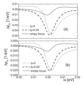
Figure 3: Change in the spectral density of the $f$ state, proportional to $\Delta dI/dV$ (see Eqs. (13), (15)) as a function of frequency at the impurity site for two values of $q$ and at the other focus, for two sets of parameters (a) $V_{s}=0.68$ eV, $\delta_{b}=0$, $E_{d}^{eff}=0.015$ eV (b) $V_{s}=0.48$ eV, $\delta_{b}=0.032$ eV, $E_{d}^{eff}=0.007$ eV. In both cases $\delta_{F}=0.04$ eV, $U=1$ eV, $T=0$.

The decrease in the intensity of the resonance at the mirage point with respect to the impurity position can be understood from Eqs. (15) and (22) and is a consequence of the destructive interference of the $42^{th}$ state of the ellipse (which lies at the Fermi level and is even under reflection through the minor axis $\sigma$) with other states which are odd under $\sigma$ (like states 32, 35, and 51): all terms contribute to the same sign to the dominant imaginary part of the sum in Eq. (22) for $R_{1}=R_{2}$, while there is a partial cancellation for $R_{1}=-R_{2}$. This interference decreases with decreasing $\delta_{F}$ and the intensity at the mirage point increases. For $\delta_{F}=0.02$ eV, $V_{s}$ should be decreased slightly to $0.63$ eV to keep the same width of the resonance, for $\delta_{b}=0$. Taking $V_{s}=0.45$ eV and increasing $\delta_{b}$ from zero to $\delta_{b}=0.035$ eV to keep the width of $\rho_{d}(\omega)$ (as above), the result for $\Delta\int d\omega\rho_{f}(\omega)(-\partial f(\omega)/\partial\omega)\sim\Delta dI/dV$ is shown in Fig. 4 for two different temperatures. At $T=0$, in comparison with the previous results for $\delta_{F}=0.04$ eV, the intensity at the mirage increased to nearly $60\%$ of that at the impurity position. At the Kondo temperature, the resonances at both positions broaden and the amplitude at the minima decrease more than $50\%$ of the zero temperature result. Most of the broadening is due to the effect of the derivative of the Fermi function, $-\partial f(\omega)/\partial\omega$. In fact, $\Delta\rho_{f}(\omega)$ at the impurity looses only $\sim 1/3$ of the intensity and broadens very little as $T$ is increased from $0$ to $0.005\ eV$.

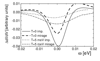
Figure 4: Change in differential conductance at both foci for two temperatures. Parameters are $V_{s}=0.45$ eV, $\delta_{F}=0.02$ eV, $\delta_{b}=0.035$ eV, $E_{d}^{eff}=0.007$ eV, $U=1$ eV, $q=0.02$.

If $\delta_{F}$ is further reduced, the space dependence of $\Delta\rho_{f}(\omega)$ is almost exactly that of the conduction eigenstate at $\epsilon_{F}$ and therefore the intensities at both foci are practically the same. However, the shape of the resonance strongly changes, and two positive contributions to $\Delta\rho_{f}(\omega)$ appear at both sides of $\epsilon_{F}$. This has been shown before for $\delta_{b}=0$, ali2 and is a consequence of the splitting of the Kondo peak in the impurity density of states $\rho_{d}(\omega)$ rap ; wil . This splitting of the Kondo peak into two peaks at both sides of the Fermi energy, which was obtained first in perturbation theory rap ; ali2 and later by exact calculation of a reduced Hamiltonian plus embedding in the rest of the system wil has been recently confirmed by numerical Wilson renormalization group calculations in a simpler system with U(1) symmetry cor . As shown in Fig. 5, this effect remains for $\delta_{b}\neq 0$, although the split peaks in $\rho_{d}(\omega)$ do not reduce to two delta functions for $\delta_{F}=0$ in this case (see Fig. 6). In Fig. 6 we also show the temperature dependence of $\rho_{d}(\omega)$ for the parameters of Fig. 4.

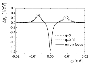
Figure 5: $\Delta\rho_{f\sigma}\sim\Delta dI/dV$ as a function of frequency for $\delta_{F}=0.001$ eV and other parameters as in Fig. 4.

So far, the experiments were done at very small temperatures ($T\cong 4$ K $\ll T_{K}\cong 50$ K), and there is no appreciable difference with the $T=0$ results. A study of the temperature dependence would confirm that the resonance is due to a many-body effect. In general (including other situations discussed below), the scale of the $T$ dependence is determined by $T_{K}$, which in turn is given by half of the with of the peak in the impurity spectral density $\rho_{d}(\omega)$. As can be seen comparing Figs. 4 and 6, for moderate $\delta_{F}$ (like $\delta_{F}=0.02$ eV), this width is larger than the width of the dip in the conduction electron spectral density $\rho_{c}(\omega)$ or in $\rho_{f}(\omega)$.

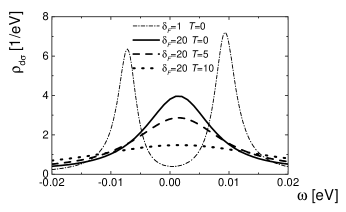
Figure 6: Impurity spectral density for several values of $\delta_{F}$ and $T$ indicated in meV inside the figure. Other parameters as in Fig. 4

The essential features of the space dependence of $\Delta dI/dV$ are very similar to that discussed previously rap ; wil and will not be reproduced here. Essentially it reflects the electron density of the conduction state at $\epsilon_{F}$, somewhat blurred out of the impurity position for $\delta_{F}\gtrsim 0.03$ eV.

In the following we use the four set of parameters which lead to a reasonable line shape at the impurity site ($\delta_{F}=0.02$ eV or $\delta_{F}=0.04$ eV, $\delta_{b}=0$ or $\delta_{b}\neq 0$) to study other situations for which the voltage dependence of $\Delta dI/dV$ has not been reported. We first consider an elliptical corral with the same eccentricity but semimajor axis reduced from $a=71.3$ Å to $a=64.6$ Å. In this case, the conduction state 35 (instead of 42) of the ellipse falls at $\epsilon_{F}$. The electronic density of this state $\left|\varphi_{35}(R)\right|^{2}$, has maxima at $R=\pm 0.4a$, displaced from the foci $R=\pm 0.5a$. Studying the negative interference at the mirage point, one expects a stronger mirage at $R_{t}=0.4a$ if the impurity is placed at $R_{i}=-0.4a$ rap . We studied two cases, with the impurity at one focus or at one maximum of $\left|\varphi_{35}(R)\right|^{2}$ for the four set of parameters mentioned above (actually, from the discussion of the previous section, one would expect a $10\%$ reduction of $\delta_{F}$, with respect to the larger ellipse, but we neglect it). For $R_{i}=-0.5a$ (impurity on focus), the resonance narrows with respect to the previous case. This is mainly due to the fact that the effective hybridization of the state at the Fermi level is proportional to $\left|\varphi_{35}(R_{i})\right|^{2}$ which is approximately $60\%$ of $\left|\varphi_{42}(R_{i})\right|^{2}$ of the larger ellipse. The total width is near $0.005$ eV for $\delta_{b}=0$ , and near $0.007$ eV for $\delta_{b}\neq 0$ (see Fig. 7 (a)). The intensity of the depression at the other focus $R_{t}=0.5a$ is roughly half of that at $R_{t}=0.4a$ at the extremum of $\varphi_{35}(R_{i})$ near that focus. In particular for $\delta_{F}=0.02$ eV (not shown), the dip in $\Delta\rho_{f}(\omega)$ at $R_{t}=0.4a$ is slightly more pronounced than that at the impurity position $R_{t}=R_{i}=-0.5a$.

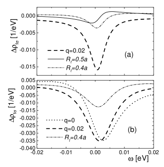
Figure 7: $\Delta\rho_{f\sigma}\sim\Delta dI/dV$ as a function of frequency at several points for an ellipse with $a=64.6$ Åand two impurity positions: (a) $R_{i}=-0.5a$ and (b) $R_{i}=-0.4a$. Other parameters as in Fig 4.

When the impurity is placed at one extremum of $\varphi_{35}(R)$, $R_{t}=0.4a$, the peak broadens with respect to the larger ellipse to $\sim 0.015$ eV for $\delta_{b}=0$, or $0.012$ eV for $\delta_{b}\neq 0$, due to the $\sim 20\%$ larger effective hybridization with the state at $\epsilon_{F}$ (see Fig. 7 (b)). As expected rap , the intensity at the mirage point $R_{t}=0.4a$, compared to the impurity point is larger in the smaller ellipse.

While the intensity of the mirage is closely related with the hybridization of the impurity with the state at $\epsilon_{F}$, the width of the peak in the impurity spectral density and hence $T_{K}$ depends on the effective hybridization with the impurity of all conduction states. For example, if in the ellipse of the original experiments one suppresses artificially the hybridization with the main odd states 32, 35, and 51, the width in $\rho_{d}(\omega)$ is reduced to roughly half its value for realistic $\delta_{F}$, while the magnitude of $\Delta dI/dV$ at the mirage point increases substantially, reaching almost the same magnitude as in the focus occupied by the impurity. The width in $\Delta dI/dV$ is less sensitive to the parameters as that of $\rho_{d}(\omega)$. As expected, this sensitivity is decreased for increasing $\delta_{F}$.

IV.2 The circular corral

In this section we study the voltage and space dependence of $\Delta dI/dV$ for a circular corral, for conditions corresponding to recent experiments man2 : a radius $r_{0}\sim 63.5$ Å, such that the degenerate $37^{th}$ and $38^{th}$ conduction eigenstates lie at the Fermi energy. In contrast to the elliptical corral, we do not use the approximate expression (22) for the conduction electron Green’s function, but the correct expansion given by Eqs. (7) and (8). The width of the resonant states is determined by the potential scattering at the boundary $W$, and its value at the Fermi energy $\delta_{F}$ is given in Table 1.

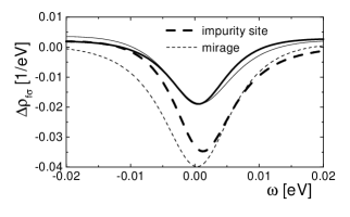
Figure 8: $\Delta\rho_{f\sigma}\sim\Delta dI/dV$ as a function of frequency for $R_{t}=R_{i}=0.146r_{0}$ (dashed line) and $R_{t}=-0.18r_{0}$ (solid line) for the circular corral. The thinner lines are the results using the approximate expression (22) changing $R_{i}$ to $0.138\ r_{0}$ and $R_{t}=-R_{i}$. Parameters are $W=7\hbar^{2}/(2m_{e}^{*}r_{0})$, $V=0.48$ eV, $\delta_{b}=0.032$ eV, $E_{d}^{eff}=0.01$ eV and $q=0.02$.

In Fig 8 we show $\Delta\rho_{f\sigma}\sim\Delta dI/dV$ for an impurity placed at a distance $0.146\ r_{0}$ to the center (corresponding to a maximum of the conduction density of states, see Table 1), for $W=7\hbar^{2}/(2m_{e}^{*}r_{0})$, and other parameters similar to Figs. 3(b) or 7. As in previous cases, an intense resonance is observed not only at $R_{i}$ but also near $-R_{i}$. The maximum of the absolute value of $\Delta\rho_{f\sigma}$ for the mirage is slightly displaced towards $0.18r_{0}$.We also show in Fig 8 the results using the approximation for the unperturbed conduction electron Green’s function $G_{s}^{0}$ based on the wave functions for the hard wall, Eq. (22). The resonance is broader in this case. This is due to the fact that with decreasing $W$, not only the maximum in real space of the conduction density of states shifts, but also the spectral weight of the resonance at $\epsilon_{F}$ near this maximum decreases, leading to a smaller effective hybridization. When $W$ is increased so that $\delta_{F}\sim 0.02\$eV, the intensity at $-R_{i}$ increases. Also when $\delta_{b}=0$ is taken, increasing $V_{s}$ the resonances broaden by $\sim 20\%$. These changes are qualitatively similar to those reported for the smaller ellipse.

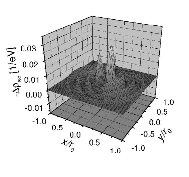
Figure 9: Conduction electron density of states at $\epsilon_{F}$ as a function of position. Other parameters as in Fig. 8.

The space dependence of the conduction density of states is shown in Fig. 9. The two clear minima near $\pm R_{i}$ can be seen, one of them corresponding to the impurity and the other to the mirage, in agreement with experiments man2 . The addition of the impurity breaks the degeneracy of the states with $m=\pm 1$ at $\epsilon_{F}$. If the zero line of the angular variable $\theta$ is aligned with the impurity, the wave function which hybridizes with the impurity has an angular dependence proportional to $\cos\theta$, and the remaining one, proportional to $\sin\theta$ does not hybridize. This has led to the proposal man2 that two independent and simultaneous mirages can be observed placing two impurities at the same distance from the center and forming an angle of $90$ degrees. While this seems in agreement with experiment, the conduction states with even $m$ (which lie out of $\epsilon_{F}$), introduce a small interaction between both channels.

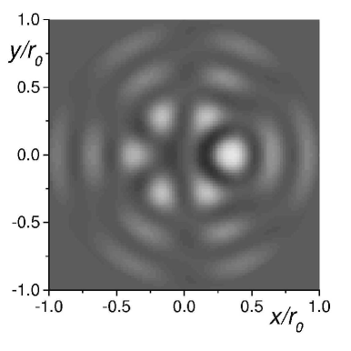
Figure 10: Contour plot of the conduction electron density of states at $\epsilon_{F}$ as a function of position for a smaller corral (see text). Parameters are $W=15\hbar^{2}/(2m_{e}^{*}r_{0})$, $V=0.45$ eV, $\delta=0.035$ eV, and $E_{d}^{eff}=0.013$ eV.

To end this section we discuss what happens when $r_{0}$ is slightly reduced in such a way that the degenerate $35^{th}$ and $36^{th}$ conduction eigenstates lie at the Fermi energy. These states have $m=\pm 3$ so that one expects five different mirages as a function of the angle $\theta$, located near $r=0.32r_{0}$, where the eigenstates for a hard wall corral are peaked. Since the value of the wave function at these extrema is nearly 3/4 times smaller than in the previous case, the effective hybridization of the impurity with the states at the Fermi energy is reduced. As a consequence, the Kondo depression observed in the energy dependence of $\Delta dI/dV$ is narrower (with a total width of $\sim$ 0.008 eV for $\delta_{F}\sim 0.02\$eV and $\delta_{b}\neq 0$), and the intensity at the mirages is smaller. In Fig. 10 we show the space dependence of $\Delta\rho_{s\sigma}\sim\Delta dI/dV$ for parameters near those of Fig. 4. A potential $W$ corresponding to harder walls (leading to $\delta_{F}\sim 0.02\$eV) than in Fig. 9 has been chosen in order that the different mirages can be clearly seen. The most intense ones are those for $\theta=\pm 120$ degrees. In addition to the five depressions in $\Delta\rho_{s\sigma}(R_{t})$ corresponding to the mirages, one can see a ring of positive $\Delta\rho_{s\sigma}$ centered at the impurity site at $R_{i}=0.337r_{0}$ and radius smaller than $r_{0}$. The intensity of this ring increases with decreasing $W$ (softer walls) and is therefore also apparent in Fig. 9. We believe that this feature is probably related with the Friedel oscillations which are observed experimentally when the impurity is placed on the clean surface knorr .

V Spin-spin correlations

The conventional view of the Kondo effect for an impurity in an ordinary metal, interprets it in terms of a magnetic screening cloud around the impurity of radius

$$\xi=\hbar v_{F}/T_{K},$$ (28)

where $v_{F}$ is the Fermi velocity. The existence of this cloud is still controversial sor ; barz ; col . Recent theoretical work has shown that the persistent current as a function of flux $j(\Phi)$ in mesoscopic rings with quantum dots changes its shape smoothly as the length of the ring $L$ goes through $\xi$ and that $jL$ is a universal function of $L/\xi$ pc ; aff .

In spite of this controversy, it is interesting to study the effect of the corral on the space dependence of spin-spin correlations. To this end we consider the correlations between the impurity spin ${\bf S}$ and that of the surface conduction states at position $r$, ${\bf s}(r)$

$$\langle{\bf S\cdot s}(r)\rangle=\sum_{j\alpha\beta\gamma\delta}\frac{\lambda^{2}}{4}\overline{\varphi}_{j}(r)\varphi_{j}(r)\langle d_{\alpha}^{\dagger}{\bf\sigma}_{\alpha\beta}d_{\beta}\cdot s_{j\gamma}^{\dagger}{\bf\sigma}_{\gamma\delta}s_{j\delta}\rangle.$$ (29)

For infinite confinement ($W\rightarrow+\infty$, $\delta_{F}=0$), exact numerical results in a reduced basis set show that the space dependence of this function follows closely the probability of the wave function lying at the Fermi level wil . However, as discussed before, this situation is not realistic.

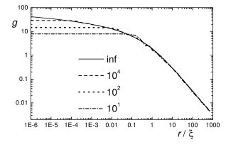
Figure 11: Function $g(r/\xi)$ (see Eq. (34)) for different symmetric limits of integration indicated inside the figure.

In the uncorrelated case $U=0$, using Wick’s theorem and the symmetry of the ground state one has:

$$\langle{\bf S\cdot s}(r)\rangle=-\frac{3}{2}\lambda\left|\sum_{j}\varphi_{j}(r)\langle d_{\sigma}^{\dagger}s_{j\sigma}\rangle\right|^{2}.$$ (30)

The saddle point approximation of the slave boson treatment of the Anderson model colb , or of the $1/N$ expansion of the Kondo model col , lead to a similar expression. Here we use Eq. (30) as an approximation for the finite $U$ problem. This amounts to an infinite partial summation of diagrams which can be separated into two pieces. The expectation value entering Eq. (30) can be related to $G_{d}(\omega)$ without further approximations using equations of motion. At zero temperature this leads to:

$$\langle{\bf S\cdot s}(r)\rangle\cong-\frac{3\lambda^{4}}{2\pi^{2}}\left|\sum_{j}\overline{\varphi}_{j}(R_{i})\varphi_{j}(r)\int^{\epsilon_{F}}d\omega\text{\rm Im}\frac{G_{d}(\omega)}{\omega+i\eta-\epsilon_{j}}\right|^{2}$$ (31)

We believe that the main qualitative features of the problem are retained by this approximation, at least for $r\lesssim\xi$ which is the relevant case for the corrals. To check this, we evaluated this expression for the case of a Kondo impurity in an ordinary three-dimensional metal, assuming (as usual in this case) that plane waves describe the conduction electrons, and (except for a multiplicative constant) $G_{d}(\omega)\sim 1/(\omega-\epsilon_{F}+iT_{K})$ por ; aga , with $T_{K}\ll\epsilon_{F}$. Calling $I(\epsilon_{j})$ the integral entering Eq. (31) and linearizing the spectrum around $\epsilon_{F}=\hbar v_{F}k_{F}$ one has:

$$\sum_{j}\overline{\varphi}_{j}({\bf R}_{i})\varphi_{j}({\bf r})I(\epsilon_{j}) \sim \int d^{3}{\bf k}\exp(i{\bf k}\cdot{\bf r})I(\hbar v_{F}k)$$

$$\sim \frac{k_{F}}{r}\int dk\sin(kr)I(\hbar v_{F}k).$$

Here the vectors are denoted by boldface (${\bf k},{\bf r}$) to distinguish them from their absolute values ($k,r$). Changing variable $z=(k-$ $k_{F})\xi$, and performing the integral in $\omega$ ($I(\hbar v_{F}k)$), we obtain except for a constant:

$$\langle{\bf S\cdot s}(r)\rangle\sim\frac{\sin^{2}(k_{F}r)}{r^{2}}g(r/\xi),$$ (33)

$$g(r/\xi)=\int dz\cos(\frac{zr}{\xi})\frac{\pi|z|/2-\ln(z)}{z^{2}+1}.$$ (34)

$g(0)$ diverges unless one introduces a cutoff at $|z|\cong k_{F}\xi=\epsilon_{F}/T_{K}$. For other values of the argument the integral can be extended to infinity at both sides, and it can be related to tabulated integrals grad . The result is:

$$g(x)=-\pi e^{x}\mathop{\rm Ei}(-x)\text{; }x\neq 0,$$ (35)

where $\mathop{\rm Ei}(x)=\int_{-\infty}^{x}dt\exp(t)/t$ is the integral exponential function. The function $g(r/\xi)$ is represented in Fig.11 for several values of the cutoff in $|$$z$$|$. As seen in the figure, this cutoff only modifies the function for small arguments. There is a crossover for $r\sim\xi$ and for $r\gg\xi$, $g(r/\xi)$ decays linearly with $r$, leading to a $1/r^{3}$ decay of $\langle{\bf S\cdot s}(r)\rangle$. The functional form of $\langle{\bf S\cdot s}(r)\rangle$ is very similar to that of the spin susceptibility suggested by Sorensen and Affleck sor ; barz for $r\lesssim\xi$. However, for $r\gg\xi$ they obtain an exponential decay. Therefore, we expect that the main features of the space dependence of the correlation function are retained by the approximation Eq. (30) for $r\lesssim\xi$.

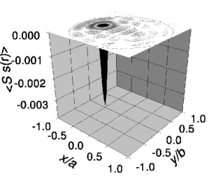
Figure 12: Correlations between the spin of the impurity and that of the conduction electrons as a function of the position of the latter. Other parameters as in Fig. 4.

In Fig. 12, we show the evaluation of Eq. (31) for the elliptical corral, with the parameters of Fig.4 and zero temperature. In contrast to $dI/dV$ or the local spectral density of states near $\epsilon_{F}$ (Fig. 4 and previous calculations for perfect confinement ($\delta_{F}=0$) wil , the spin correlations do not recover substantially at the empty focus, although still faint features related with the conduction state at the Fermi level ($j=42$) are still discernible.. The ratio of the spin correlations at both foci is $\sim 1/170$. Note that from $T_{K}$ and $v_{F}$ for surface electrons in the mirage experiments, one gets $\xi\sim 90$ Å, slightly larger than the distance between foci. As it is clear from the calculation above, for $r\lesssim\xi$ all conduction states (also those at high energies) contribute to the spin-spin correlations. Therefore, the destructive interference near the empty focus is larger than in the case of $dI/dV$, in which mainly unperturbed conduction states near $\epsilon_{F}$ are sampled. The participation of high energy electrons in the formation of the singlet ground state has been stressed recently col .

VI Summary and discussion

We have studied the 2D Green’s function for free electrons, subject to a potential that simulates a continuous circular corral. We disregarded the hybridization with bulk states at the boundary of the corral. In scattering theories, an imaginary part is introduced for the phase shift to take into account this effect in phenomenological way cro ; aga ; fie , and this leads to loss of intensity at the mirage point when an impurity is introduced in the corral. In our theory this loss of intensity comes as a result of quantum interference, as explained in Section IV. Although the density of states is continuous in space and energy, the energy dependence of the Green’s function at low energies can be written as a sum of discrete poles, representing resonant states. This property is expected to persist for more realistic potentials which might include hybridization with bulk states or individual atoms at the boundary at the corral cal . The introduction of a width $\delta_{i}$ of each resonance is the main difference with a calculation assuming a hard wall corral. The energies $\epsilon_{i}$ and the space dependence of the density of states inside corral are well described by the calculation assuming hard walls, but the magnitude of the latter is somewhat overestimated. Our model leads to a width of each resonance $\delta_{i}$, which is to a first approximation, proportional to its energy $\epsilon_{i}$ . We must warn however that at least above the Fermi energy, the surface states have an intrinsic width, even in absence of the corral hub . Thus, while we expect that $\delta_{i}$ can be reduced for example by depositing a second line of atoms at the boundary of the corral, there are probably intrinsic limits to this reduction. Another shortcoming of our one-body calculation is that actually the effective mass depends on energy. Photoemission experiments suggest a flattening of the dispersion above $\epsilon_{F}$ hub . This is also apparent in the comparison of experimental energy levels for a circular corral an those of a hard wall calculation cro and persists in our results for soft boundaries.

The expansion as a sum of discrete poles of the conduction electron Green’s function is a convenient starting point for a perturbative treatment of the Anderson model that describes the physics when a magnetic impurity is introduced inside the corral. The line shape of the change in differential conductance $\Delta dI/dV$ and the relative intensity at points distant from the impurity (where a “mirage” of the impurity is observed man ) is very sensitive to $\delta_{i}$. This sensitivity is reduced but persists if an important intrinsic width $\delta_{b}$ of the impurity level due to direct hybridization with bulk states is introduced. A smaller $\delta_{i}$ leads to a stronger intensity at the mirage point, and the space dependence tends to that of the conduction state at $\epsilon_{F}$. However, for very small $\delta_{i}$ the line shape (voltage dependence), is strongly distorted and two peaks of positive weight of $\Delta dI/dV$ appears at moderate non-zero voltages. The line shape and its width depend also on the particular conditions of the experiment. This fact includes the case of the clean surface, as observed experimentally man , and calculated before ali2 . A larger width and more intense resonance is expected when the wave function of the conduction state which lies at the Fermi energy has a stronger amplitude at the impurity.

While the space dependence of $\Delta dI/dV$ is determined only by the conduction electron Green’s function in absence of the impurity (see Eqs. (13) and (15)), the voltage dependence is very sensitive to the impurity Green’s function. Most previous theories either assume or fit this line shape por ; aga ; fie or are unable to explain the observed one because $\delta_{i}=0$ was assumed hal . Also while numerical diagonalization with $\delta_{i}=0$ and a reduced basis set show spin-spin correlations which remind the conduction state at the Fermi level wil , we obtain using additional approximations discussed in Section V, that no appreciable projection to the mirage point is present in these correlations. This is due to the fact that the screening of the spin involves conduction states far from the Fermi energy $\epsilon_{F}$, while $\Delta dI/dV$ selects states near $\epsilon_{F}$. These experiments seem unable to settle the still controversial issue of the Kondo cloud sor ; barz ; col . Instead, a crossover as a function of size is expected in mesoscopic rings pc ; aff .

Our many-body theory is able to explain the main features of the space and voltage dependence of $\Delta dI/dV$ in several experiments involving the quantum mirageman ; man2 and predictions for other geometries and experimental conditions were made. While it would be interesting to test this predictions and study the effects of temperature, the theory has some limitations. A real Co atom added to a Cu(111) surface has degenerate localized 3d levels with strong correlations. We have taken only one d orbital with a moderate on-site Coulomb repulsion $U=1$ eV to be able to use the perturbative approach. We believe however that these shortcomings affect quantitative details but do not invalidate our conclusions. Previous results using larger values of $U$ and a different technique led to results very similar to the perturbative ones wil . A Co atom also has extended 4s and 4p electrons, which should have a large hopping to the STM tip when it is near the impurity. This should affect the amplitude of $\Delta dI/dV$ at moderate distances to the impurity. This effect has so far been neglected in the theories of the mirage effect.

References

- (1) D.M. Eigler and E.K. Schweizer, Nature (London) 344, 524 (1990).
- (2) M.F. Crommie, C.P. Lutz, and D.M. Eigler, Science 262, 218 (1993).
- (3) E.J. Heller, M.F. Crommie, C.P. Lutz, and D.M. Eigler, Nature (London) 369, 464 (1994).
- (4) H.C. Manoharan, C.P. Lutz, and D.M. Eigler, Nature (London) 403, 512 (2000).
- (5) H.C. Manoharan, PASI Conference, Physics and Technology at the Nanometer Scale (Costa Rica, June 24 - July 3, 2001).
- (6) S.L. Hulbert, P.D. Johnson, N.G. Stoffel, W.A. Royer, and N.V. Smith, Phys. Rev. B 31, 6815 (1985).
- (7) A.A. Aligia, Phys. Rev. B 64, 121102(R) (2001). (cond-mat/0101082)
- (8) D. Porras, J. Fernández-Rossier, and C. Tejedor, Phys. Rev. B 63, 155406 (2001).
- (9) M. Weissmann and H. Bonadeo, Physica E (Amsterdam) 10, 44 (2001).
- (10) K. Hallberg, A.A. Correa, and C.A. Balseiro, Phys. Rev. Lett. 88, 066802 (2002).
- (11) A.A. Aligia, Phys. Status Solidi (b) 230, 415 (2002). (cond-mat/0110081)
- (12) G. Chiappe and A.A. Aligia, Phys. Rev. B 66, 075421 (2002).
- (13) O. Agam and A. Schiller, Phys. Rev. Lett. 86, 484 (2001).
- (14) G.A. Fiete, J. S. Hersch, E. J. Heller, H.C. Manoharan, C.P. Lutz, and D.M. Eigler, Phys. Rev. Lett. 86, 2392 (2001)..
- (15) N. Knorr, M. A. Schneider, L. Diekhöner, P. Wahl, and K. Kern, Phys. Rev. Lett. 88, 096804 (2002).
- (16) M. Plihal and J.W. Gadzuk, Phys. Rev. B 63, 085404 (2001).
- (17) G. García Calderón, Nucl. Phys. A 261, 130 (1976).
- (18) See for example J.R. Taylor, Scattering Theory: the quantum theory of non-relativistic collisions (Wiley, New York, 1972).
- (19) M. Abramowitz and I.A. Stegun, Handbook of mathematical functions (Dover, New York, 1965).
- (20) A. Schiller and S. Hershfield, Phys. Rev. B 61, 9036 (2000).
- (21) A. Euceda, D.M. Bylander, and L. Kleinman, Phys. Rev. B 28, 528 (1983).
- (22) Experimentally for Å and finite , while we have taken for . Then, actually we have to start with a slightly larger effective mass to reach the experimental condition. However, since the difference is small, practically it does not modify our results and we neglect it.
- (23) O.Újsághy, J. Kroha, L. Szunyogh, and A. Zawadowski, Phys. Rev. Lett. 85, 2557 (2000).
- (24) T.A. Costi, J. Kroha, and P. Wölfle, Phys. Rev. B 53, 1850 (1996).
- (25) K. Yosida and K. Yamada, Prog. Theor. Phys. Suppl. 46, 244 (1970); Prog. Theor. Phys. 53, 1286 (1975); K. Yamada, ibid 53, 970 (1975).
- (26) B. Horvatić, D. Šokčević, and V. Zlatić, Phys. Rev. B 36, 675 (1987).
- (27) R. N. Silver, J. E. Gubernatis, D. S. Sivia, and M. Jarrell, Phys. Rev. Lett. 65, 496 (1990).
- (28) A. Levy-Yeyati, A. Martín-Rodero, and F. Flores, Phys. Rev. Lett. 71, 2991 (1993).
- (29) H. Kajueter and G. Kotliar, Phys. Rev. Lett. 77, 131 (1996).
- (30) A.A. Aligia and C. R. Proetto, Phys. Rev. B 65, 165305 (2002).
- (31) A.A. Aligia, Phys. Rev. B 66, 165303 (2002).
- (32) M. Weissmann and A.M. Llois, Phys. Rev. B 63, 113402 (2001).
- (33) To find numerically the poles of we started form the case (for which poles of lie between two consecutive poles of ) and then increased slowly to the desired value. Doing so, we can trace continuously the position of these poles in the complex plane.
- (34) G.D. Mahan, Many Particle Physics (Plenum, New York, 1981).
- (35) In general, the unperturbed Green’s function (retarded or time-ordered) for electrons can be written as , where labels all one-electron eigenstates in absence of the impurity and the time-ordered = sgn = sgn. Then, for real , Im = sgn. The retarded Green’s functions have the same form removing the sign (sgn) functions.
- (36) P. Cornaglia and C.A. Balseiro, 66, 174404 (2002).
- (37) E.S. Sorensen and I. Affleck, Phys. Rev. B 53, 9153 (1996).
- (38) V. Barzykin and I. Affleck, Phys. Rev. B 57, 432 (1998).
- (39) P. Coleman, cond-mat/0206003
- (40) I. Affleck and P. Simon, Phys. Rev. Lett. 86, 2854 (2001).
- (41) P. Coleman, Phys. Rev. B 29, 3035 (1984).
- (42) I.S. Gradshteyn and I.M. Ryshik, Table of Integrals, Series and Products (Academic Press, New York, 1965).