Low Temperature Properties of the Random Field Potts Chain

Abstract

The random field $q$-States Potts model is investigated using exact groundstates and finite-temperature transfer matrix calculations. It is found that the domain structure and the Zeeman energy of the domains resembles for general $q$ the random field Ising case ($q=2$). This is also the expected outcome based on a random-walk picture of the groundstate. The domain size distribution is exponential, and the scaling of the average domain size with the disorder strength is similar for

$q$ arbitrary. The zero-temperature properties are compared to the equilibrium spin states at small temperatures, to investigate the effect of local random field fluctuations that imply locally degenerate regions. The response to field perturbations (’chaos’) and the susceptibility are investigated. In particular for the chaos exponent it is found to be 1 for $q=2,\ldots,5$. Finally for $q=2$ (Ising case) the domain length distribution is studied for correlated random fields.

I introduction

Adding disorder to random magnets creates new effects one the prime examples being the random field Ising model (RFIM) review ; rfim-rieger . Since the randomness couples directly to the order parameter one has interesting physics in the groundstate (GS) properties rfim-gs ; gs1 ; gs2 ; gs3 , already. With a finite temperature the disordering effects of entropy and local fields compete.

The purpose of this article is to explore the generalization or extension of the one-dimensional RFIM to the one-dimensional random-field Potts model. The 1d RFPM is defined on a chain of $L$ spins (with periodic boundary conditions being used here) where each spin site can be in one of $q$ states. The Hamiltonian is given by

$${\mathcal{H}}=-J\sum_{\langle i,j\rangle}(q\delta_{\vec{\sigma_{i}},\vec{\sigma_{j}}}-1)-\sum_{i}h_{i}(q\delta_{\vec{\sigma_{i}},\vec{\alpha_{i}}}-1)$$ (1)

where $\langle i,j\rangle$ are nearest-neighbour pairs and $\delta_{\sigma,{\sigma}^{\prime}}$ the Kronecker-delta, i.e., $\delta_{\sigma,{\sigma}^{\prime}}=1$ for $\sigma={\sigma}^{\prime}$ and $\delta_{\sigma,{\sigma}^{\prime}}=0$ otherwise . The vector $\vec{\alpha}_{i}$ is a unit vector pointing randomly in one of the $q$ spin directions and $h_{i}$ is the local field strength which is chosen either constant or randomly distributed. In the numerical computations presented below we have used a Gaussian distribution for the random fields with $\langle h_{i}\rangle=0$ and $\langle{h_{i}}^{2}\rangle={h_{r}}^{2},$ such that $h_{r}/J$ is a measure for the strength of the disorder, except at finite $T$ where fields are uniformly distributed between [$-\delta,+\delta$]. In the following we denote the one-dimensional versions of the RFIM and the RFPM with RFIC(random field Ising chain) and RFPC(random field Potts chain).

Our approach is to explore the RFPC by three different techniques. We compute the exact GS by using a shortest path methodgs1 ; gs2 ; gs3 . This is a generalization of an idea that allows to find the GS of the RFIC, and can be understood as the zero-temperature limit of the transfer matrix computation of the equilibrium spin state. This is also employed here, to compare that state with the GS. Finally we resort to a qualitative description in terms of a random-walk (RW) picture of the groundstate. T his is also an extension of the RFIC case, where an earlier paperSchroeder01 presented a RW description of the exact groundstates.

There is rather little work on the RFPC with the exception of trivial field distributions chains ; Binder . Thus it is worth to recapitulate some of the features of the RFIC or the reasons why it still receives some attention. Due to the fact that the model is one-dimensional one could expect that the basic magnetization properties are more or less trivial. It turns out to be so, however, that in particular for binary random field distributions ($h_{i}=\pm h_{r}$) these have very peculiar propertiesBruinsma83 ; Andelman86 . The equation for the local magnetization can be considered as a 1d dynamical system with, for suitable parameters, a multifractal probability distributionBene88 . For the RFPC this is perhaps also the case, generalized to higher dimensions if $q>2$. In this article we omit such considerations for the sake of the equilibrium and groundstate properties.

One of the points of an exact solution for the GS is that it can be investigated how exactly the introduction of a small, finite temperature breaks up the GS. For the RFPC it is more or less trivial that the overlap between the GS and the $T>0$ state stays close to one, contrary to e.g. spin glasses where this question may still be open to a debate. However, it is of interest to study how exactly the GS is modified by the “easy” excitations. These are, as discussed below, related to the almost degenerate regions of the GS. The equilibrium state is also of interest as the asymptotic one for out-of-equilibrium processes. In such one-dimensional systems the domain walls undergo activated dynamics, in particular the RFIC ones perform Sinai walks Bouchaud90 ; LeDoussal .

The structure of the rest of the paper is as follows. First we overview, in section II, the theoretical expectations for the groundstate properties and outline qualitatively the consequences for perturbations from a given GS, whether by temperature or by changing the local fields (by random shifts or by an uniform applied field). Section III is devoted to exact numerical studies of the RFPC. In Section IV the temperature is switched on, and the effect of entropy on the domain structure is analyzed. Section V contains a brief numerical study of the effect of correlated fields. Finally, Section VI finishes the paper with conclusions. The numerical techniques are discussed in the Appendices.

II Random Walks: decomposition of the groundstate

We have earlier presented a way to divide the sequence of random fields $h_{i}$ for the RFIC in such a way so that one can understand the ensuing domain structure Schroeder01 . The idea is to look at trial random walks: start from a test site, and follow the sum of the random fields left/right (an arbitrary choice). Each of such trials constitutes either an absorbing or non-absorbing one. The terms describe the fact that trials are random walks with absorbing boundaries. One boundary results in an excursion of the RW which is such that enough Zeeman energy ($2J$) is accumulated to form a domain, but if the other one is met first the try is finished and a new one is started. Since the RW’s are independent, the GS factorizes. Mathematically such excursions are given by the following rules. An $absorbing$ excursion ($ae$) is a sequence $\mathcal{S}$ of spins starting at some lattice site $i$ and ending at $j\geq i$, with the field sum $|\sum_{i\in{\mathcal{S}}}h_{i}|$ for the first time becoming greater or equal to $2J$. On the other hand a sequence $\mathcal{S^{\prime}}$ of spins from $i$ to $j\geq i$ is a non-absorbing excursion ($nae$) if $0<\bar{\sigma}\sum_{l=i}^{j}h_{l}<2J$ $\forall i<k<j$ ; where $\bar{\sigma}=\pm 1$ is the orientation of the spins within the preceding $absorbing$ excursion.

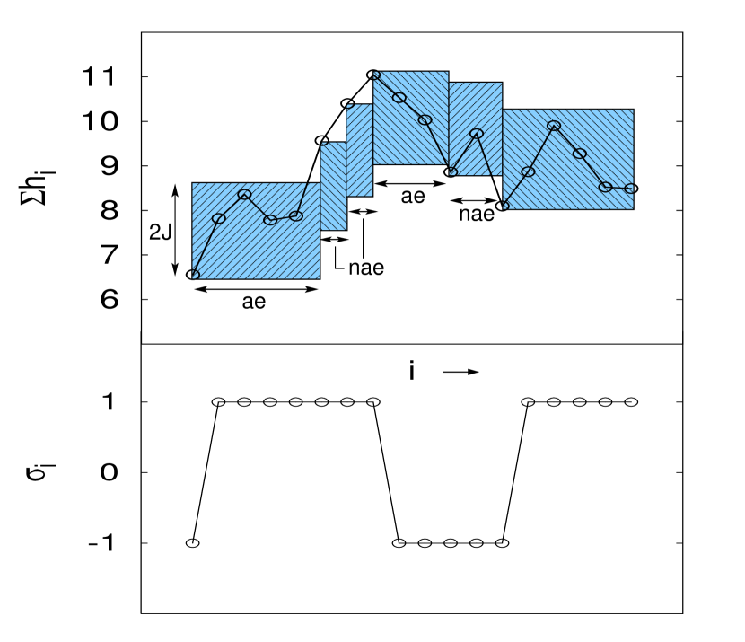
Figure 1: Random walk picture for the RFIC domains. The upper part of the figure shows the field sum $\sum h_{i}$ at each of the spin sites (starting from the left) and the lower part depicts the corresponding domain structure. The random walk starts a $non-absorbing$ (nae) excursion as soon as it leaves the shaded region of height $2J$(for details see text).

As shown in Figure 1 for each domain one has at least one such absorbing RW (it can contain more than one such large fluctuation) and it will be bounded by the next opposite absorbing RW’s on each side. The rules to be followed are: (1) Determine an absorbing excursion ${\mathcal{S}}_{0}$ for a given field configuration. If it starts at site $i_{0}$ and ends at $j_{0}$, and $\bar{\sigma}$ is the sign of its field sum, then $\sigma_{k}=\bar{\sigma}$ $\forall k\in{\mathcal{S}}_{0}$. (2) Starting from $j_{0}+1$ find all non-absorbing excursions until the next absorbing excursion ${\mathcal{S}}_{1}$ (from $i_{1}$ to $j_{1}$) is found, whose field sum is by definition opposite in sign to the preceding one. The sites $k$ belonging to the non-absorbing excursions have the same orientation $\sigma_{k}=\bar{\sigma}$ as those within ${\mathcal{S}}_{0}$. The orientation of the spins at sites $l$ within ${\mathcal{S}}_{1}$ is opposite to the later one, $\sigma_{l}=-\bar{\sigma}$. (3) Starting at $j_{1}+1$ the search (2) for the next absorbing excursion then leads to the overall GS.

This picture explains also, for binary random fields $h_{i}=\pm h$, the degeneracy of the RFIC. For our purposes it is more important to note that for any kind of perturbations it implies that there are three processes, domain wall-shifts, destruction and creation of domains, that follow naturally from the sequence of RW’s. If one changes the local random fields some of the absorbing excursions become non-absorbing, and thus domains are destructed while new ones may ensue if some non-absorbing ones become absorbing. These are in principle easy and in practice cumbersome (since one needs to be concerned with the exact first passage properties of the perturbed field distributions or random walk step length distributions) to compute for each process. Moreover, the normal outcome is that the domain-walls are shifted. The major results that follow for the RFIC from the RW picture concern the domain structure and optimization. The domain magnetic (Zeeman) energy scales linearly with domain size in contrast to the Imry-Ma argumentImry75 . The domain size distribution is exponential, and for $h_{r}\ll 1$ the Imry-Ma result $\langle l_{d}\rangle\sim 1/h_{r}^{2}$ is recovered since both the contributions from the non-absorbing walks and the absorbing ones that contribute to the domain length scale with $1/h_{r}^{2}$. Thus for the RFPC it will be interesting to compare both the domain structure and the Zeeman energy,

$$H_{Z}=\sum_{i\in{\mathcal{D}}}h_{i}(q\delta_{\vec{\sigma_{i}},{\vec{\alpha_{i}}}}-1).$$ (2)

For the Potts model one can use the same thought experiment: assume the spin $\sigma_{i}=q^{\prime\prime}$, and look for “$absorbing$ excursions”. Now, in contrast to the $q=2$-case the general RFPC is more complicated. For each of the other $q^{\prime}\neq q^{\prime\prime}$ one can follow, analogously to the RFIC, the random walk that results from three steps: 1) null step (local field aligned to other direction than $q^{\prime}$ and $q^{\prime\prime}$), 2) positive and 3) negative steps. One has $q-1$ such trial walks, with the elementary step directions being correlated or shared. These follow “partial” sums of local random fields, according to the rules 1) - 3). Thus an analogy of the RFIC results in studying the first passage properties of a $q-1$ dimensional space. Either one of the coordinates is increased, or all of them are decreased ($q^{\prime\prime}$-step) at the same time. One is interested in the first-passage through one of the sides of a hyper-cube in $q-1$ -dimensions, ie. across the plane where $q^{\prime}=2J$. The walk starts in the immediate vicinity of the corner $(0,\dots,0$) of the hyper-cube. The simplest complication that arises over the $q=2$, RFIC case is that for each trial walk that compares any of the spin orientations and the original one there are “empty” steps consisting of local fields aligned with the other $q-2$ possibilities. This implies that the typical domain length might simply scale with $q$, as borne out later by the numerics.

There are two further complications compared to the RFIC, both resulting from the fact that the optimization can not be done as straightforwardly as in the RFIC due to the factorization of the landscape to absorbing and non-absorbing excursions. Namely, for $q>2$ the process is slightly non-local. Consider the $q=3$ case, and assume that spin $i$ has $q^{\prime}=1$. If a large fluctuation is found by following the appropriate partial sum of the $q^{\prime}=2$-orientation, and the next one is of $q^{\prime}=3$-kind, one has to consider whether it is energetically more favorable to create a $2$-domain, a $3$-domain, or both, since the number of domain walls created can be lowered by omitting in this example the $2$-domain. One can also use the argument the other way: if a large $3$-fluctuation exists, it is possible to create a $2$-domain since one of the domain walls is free. The following structure 1 1 1 1 3 3 3 of total energy $E_{i}$, is changed into 1 1 1 2 3 3 3 of energy $E_{f}$ by flipping a single spin $\bf{1}\rightarrow\bf{3}$ (the local random field $h_{i}=h$ directed along $\vec{\alpha}$ = 3 at the flipped site). The latter configuration would be more favourable than the former one if, $E_{f}<E_{i}$, yielding $h>J$. This shows that the minimum Zeeman energy of a domain of length 1 should at least be $J(q-1)$.

III Ground State Properties

III.1 Correlations among the successive domains and the evolution with increasing disorder

As noted above the sequence of domains is complicated due to the joint optimization. The easiest quantity is to compare the probability that the third domain from the original one is of the same orientation as the first one. We calculate the probability $P_{\sigma}(q)$ of finding the every third domain (${\mathcal{D}}_{i+2}$) to be the same or different as the first (${\mathcal{D}}_{i}$) one. In absence of any correlations among the successive domains one should expect the probability ${P}_{\sigma}^{nc}(q)$ of obtaining ${\mathcal{D}}_{i+2}$ same or different with respect to ${\mathcal{D}}_{i}$ to be,

$${P}_{\sigma}^{nc}(q)=\left\{\begin{array}[]{cll}\frac{1}{q-1}&,\mathrm{for}&{\mathcal{D}}_{i}={\mathcal{D}}_{i+2}\\ \\ \frac{q-2}{q-1}&,\mathrm{for}&{\mathcal{D}}_{i}\neq{\mathcal{D}}_{i+2}\end{array}\right.$$ (6)

Figure 2: Left: Probability of obtaining every third domain ${\mathcal{D}}_{i+2}$ same or of different as the first ${\mathcal{D}}_{i}$. The continuous lines represents the no-correlation probability function ${P}_{\sigma}^{nc}(q)$. Inset : The ratio of ${{P}_{\sigma}^{nc}(q)}/{P_{\sigma}(q)}$ means the third domain is the same as the first one. The system size $L=10^{5}$ and the number of configurations 20000.

We carried out computations with the Shortest Path Algorithm (see Appendix A) for $q=$2, 3, 4, 5 states, with the field strength $h_{r}=0.05$. It is easy to see that ${P_{\sigma}(q)}$ deviates some from the ${P}_{\sigma}^{nc}(q)$. Evidently, the system prefers to have the third domain different from the first one. One can put this in two ways: creating a 121 configuration costs more energy, on one hand, and on the other hand as noted before one can add a domain at the expense of a single domain wall between two others (131 becoming 1231).

Figure 3: Evolution of groundstate with increasing disorder strength $h_{r}$ for $q$ = 5.

The evolution of the domain structure with increasing field amplitude $h_{r}$ differs fundamentally from the same phenomena in the RFIC. New domains can be created in-between two earlier ones at a smaller cost ($2J$ instead of $4J$). Figure 3 depicts the evolution of the GS domains for a $q=5$ states sample with identical configuration of the random direction of the local fields but increasing disorder $h_{r}=$ 0.05, 0.07, 0.15. The large domains are split into smaller fragments, mostly at their boundaries.

III.2 Distribution of domain length and Zeeman energy

To compare with the $q=2$ or RFIC case we now used a larger system size of $L$ = 100000, with $n=10^{5}$ samples. Figure 4 shows the numerical results for the accumulated Zeeman energy $H_{Z}$ as a function of domain length $l_{d}$ for different field amplitudes $h_{r}$. It easy to see that all $\langle H_{Z}\rangle$ versus $l_{d}$ curves can be asymptotically (except for the smaller $l_{d}$ region) fitted to a straight line of the formSchroeder01

$$\langle H_{Z}\rangle=qJ+d_{q}h_{r}^{\gamma}l_{d}.$$ (7)

Here the coefficient $d_{q}$ grows roughly logarithmic for $q<15$.

Figure 5 shows the mean domain length $\langle l_{d}\rangle$ for different values of $q$ as a function of the field amplitude $h_{r}$. The data along the x-axis for $q=$ 3, 4, 5 are shifted by factors 2, 4 and 8 respectively. In the limit $h_{r}\ll J$ the data fits quite well with the Imry-Ma scalingImry75 $\langle l_{d}\rangle\sim 1/h_{r}^{2}$. The prefactor of the domain length is (see the inset of Figure 5), except for $q=3$, linearly dependent on $q$. Figure 6 finally shows the scaling plots of the probability distribution P($l_{d}$) of the domain lengths. Apart from the initial part, the distribution decays exponentially. We may therefore conclude that in spite of the slight correlations in the domain structure, the RFPC obeys the same scalings in the GS as the RFIC.

Figure 4: Log-log plot of the mean Zeeman energy as a function of domain length $l_{d}$. The disorder strength $h_{r}=$ 0.20, 0.15, 0.10, 0.09, 0.08, 0.07, 0.06, 0.05, 0.04, 0.03 from top to bottom in all the subplots.

Figure 5: Mean domain length as a function of $h_{r}$. The straight lines are fits to the function $f(x)=ax^{-2}$ where the coefficient $a=$6.99, 6.57, 6.89 and 7.39 respectively for $q$ = 2, 3, 4 and 5. The fit works well for smaller $h_{r}$ but deviates for larger amplitudes. Inset: The average domain length $\langle l_{d}\rangle$ as a function of $q$. The straight line is a linear fit with slope 201.88.

Figure 6: Scaling plot of the domain length probability distribution $P(l_{d})$. The data are shifted by 7, 14, 21 units along the x-axis for $q=$ 3, 4, 5, respectively. Inset: Unscaled plot of $P(l_{d})$ for $q=5$. The labels refer to the disorder strength $h_{r}$.

III.3 Response to constant external field

In the presence of an external field favoring one of the spin orientations via an additional term $h\sum_{i}(q\delta_{\vec{\sigma_{i}},\vec{\alpha_{i}}}-1)$ in the Hamiltonian($\vec{\alpha_{i}}$ arbitrary but fixed and the same for all sites), the magnetization becomes of course non-zero. The ground state magnetization is computed as

$$m_{a}={\frac{1}{N}}\sum_{i=1}^{N}\left(\frac{q\delta_{\vec{\sigma_{i}},\vec{a}}-1}{q-1}\right).$$ (8)

in a particular direction $\vec{a}$ (here $a\in[1,..,q])$ for $q$ different states. Now for a small field strength ($h_{r}\ll J$) in an infinite system one has

$${m}_{\infty}(h)\sim h.$$ (9)

For a finite system the corresponding finite-size scaling relation can be obtained as followsRieger96 ; Bray85 . In the GS the Zeeman Energy of a block of spins of size $L$ is

$$E_{Z}\sim Lh.$$ (10)

Further the random field (variance $h_{r}$) energy of the block is

$$E_{RF}\sim L^{1/2}h_{r}.$$ (11)

For a non-zero $h$ one would expect $m_{L}(h)h^{-1}$ to be a function of the dimensionless ratio of $E_{Z}$ and $E_{RF}$ only, yielding

$$m_{L}(h)=h\tilde{m}(L^{1/2}h/h_{r})$$ (12)

with

$$\tilde{m}(x)\sim\left\{\begin{array}[]{cl}\mbox{const.}&\mbox{for $x\gg 1$}\\ \\ 1/x&\mbox{for $x\ll 1$}\end{array}\right.$$ (16)

Eq. (12) can once again be written as,

$$m_{L}(h)=L^{-1/2}\bar{m}(L^{1/2}h/h_{r})$$ (17)

with $\bar{m}(x)=$ const. for $x\gg 1$ and $\bar{m}(x)=1/x$ for $x\ll 1$.

Figure 7: Ground state magnetisation for $q=$ 2, 3, 4, 5, respectively. The exponent $\nu=1.0$(for all $q$) follows from the fit to $f(x)=bx^{\nu}$, which is also verified by the data collapse according to Eq. (16).

The system is subjected to a constant external field $h$ in a fixed direction $\vec{a}=1$ to evaluate $m_{a}(S,h)$ for a sample $S$ with some given realization of random fields. To start, $h=0.0001$, and the GS magnetization is computed. Then the field is increased after averaging 1000 samples, until saturation. Here $h_{r}=0.1$, $L\in\{5000,10000,20000,40000,80000\}$ while $h$ is in the interval [0.0001, 0.03]. For smaller systems one has to use higher values of $h_{r}$, since otherwise a single domain may percolate.

III.4 Chaos Exponent

A slight variation of the random fields in each sample gives rise to “chaos”. In the case of the RFIC or RFIM in general this has already been studiedChaos ; Alava98 . There the general behavior is such that for small amplitudes $\delta$ of the local perturbation the overlap between the new and the old GS remains considerable, and the difference is a smooth function of $\delta$. This is easy to see if one considers the RW factorization of the GS: a variation of the local fields gives rise to a new RW, in superposition with the original one. In the limit $\delta\rightarrow 0$ this has only minute effects except for barely absorbing walks and barely non-absorbing ones that can be affected if $\delta$ is large enough.Thus the average overlap $q$ is linear for the RFIC in $\delta$. Next we look at the chaos properties in the RFPC.

Figure 8: Scaling plot of the overlap correlation function $C_{\delta}(r)$ versus $r\delta$. Data are averaged over 1000 samples for each perturbation strength $\delta$ with fixed system size $L=10^{5}$ and the disorder strength is fixed at $h_{r}=0.05$.

To modify the initial random fields $h_{i}$ at each site $i$ they are replaced by ${h_{i}}^{{}^{\prime}}=h_{i}+\delta{\tilde{h}}$. As before, $h_{i}$ and also $\tilde{h}$ follow Gaussian distributions and the parameter $\delta$ measures the strength of the perturbation. Denoting ${\vec{\sigma}_{i}^{0}}$ and ${\vec{\sigma}_{i}^{\delta}}$ to be the unperturbed and perturbed ground state at site $i$ respectively, the ground state overlap correlation function up to a distance $r$ is defined by

$$C_{\delta}(r)={\left[{\frac{1}{N}}\sum_{i=1}^{N}{\Delta({\vec{\sigma}_{i}^{0}},{\vec{\sigma}_{i+r}^{0}})}{\Delta({\vec{\sigma}_{i}^{\delta}},{\vec{\sigma}_{i+r}^{\delta}})}\right]}_{av}$$ (18)

with

$$\Delta(\sigma,{\sigma}^{\prime})=2\delta_{\sigma,{\sigma}^{\prime}}-1.$$ (19)

In the limit $N\rightarrow\infty$ one would expect a scaling form

$$C_{\delta}(r)\sim\tilde{c}(r/\xi(\delta))$$ (20)

with

$$\xi(\delta)\propto\delta^{-1}.$$ (21)

In Figure 8 we show the results of our calculation of the GS overlap correlation function $C_{\delta}(r)$. $r$ is varied from 4 up to 160 for each perturbation strength $\delta$. The obtained data collapse agrees quite well with the argument above.

IV Domains at finite temperature

IV.1 Changes with the introduction of a finite temperature

For $T>0$ we calculated the expectation values $\langle\sigma_{i}\rangle$ using the transfer matrix technique Bruinsma83 ; Crisanti93 as described in Appendix B. The domains start “melting”, i.e. the overlap with the GS, $\langle\sigma_{i}\sigma_{i,GS}\rangle$, decreases, as the temperature is switched on from $T=0$. The effect of temperature is similar to a random field perturbation in the sense that both should play a role in particular where the fluctuations in the random landscape (absorbing/almost absorbing walks) make it the easiest. On the other hand the effect of temperature is not limited to those regions, only. Next we compare the finite temperature and GS configurations to illuminate the $T>0$ physics.

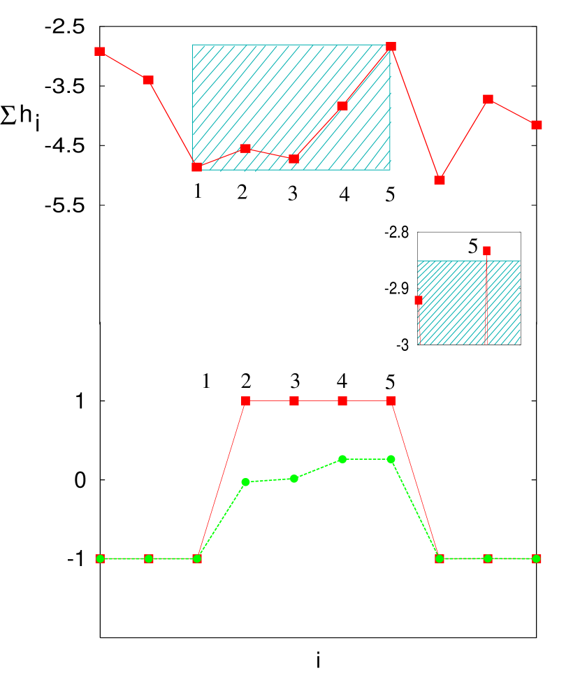
Figure 9: Destruction of a GS domain for $T>0$ in the RFIC. The upper part of the figure shows the field sum $\sum_{i}h_{i}$ in the neighbourhood of spin $i=1,...,5$, the lower part the corresponding ground state and a $T>0$ state. The reason why this domain melts at relatively low temperature is indicated in the middle part: The field sum of spin 5 is just outside the shaded area(see text).

In Figure 9 we represent the destruction of a domain for a system of size of $L$= 400 and $h_{r}$ = 0.7, as the temperature is raised to 0.2 from $T=0$. The random field distribution is uniform in the interval $[-1,1]$. The zero temperature domain from $i$ = 2 to $i$ = 5 is due to a single absorbing excursion, depicted by the large shaded region in the upper part of the Figure 9. The inset in the middle part shows the sensitive region at $i$ = 5, where the field sum just crosses the absorbing boundary. As the temperature is increased from zero, the entropy gives weight to states where the whole region or much of it is flipped, to the $\sigma=-1$ state instead of +1.

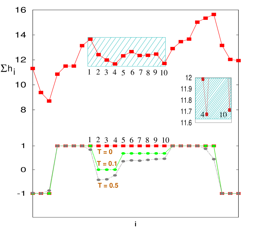
Figure 10: Creation of a fluctuation for $T>0$ (RFIC). The upper part of the figure shows the field sum $\sum_{i}h_{i}$ in the neighbourhood of spin $i=1,...,10$, the lower part the corresponding ground state and two $T>0$ states. The reason why this domain melts at relatively low temperature is indicated in the middle part: The field sum of spin 4 and 10 are very close to the absorbing boundary (see text).

Figure 10 shows the melting of a GS domain at $T=0.1$ for a system of $L$ = 400 and strength of disorder $h_{r}$ = 1.0 (the distribution of local fields is again uniform in [-1,1] ). Now the sum-of-fields random walk in the GS from $i$ = 1 to 10 is actually part of a non-absorbing excursion inside the embedding domain with $\sigma=-1$. It is however susceptible to the introduction of temperature (note the spins $i=$ 4 and 10 where the RW is closest to creating a domain, in the inset).

At a finite temperature the sites 2, 3, 4 form a “new domain” with $\sigma=-1$. This new domain contains only one part of the RF fluctuation, from 1 to 4.

To further investigate the melting of a GS domains at finite temperatures, an overview of the GS and equilibrium configurations at finite temperatures is shown in Figure 11. The calculations for each temperature including the GS are carried out for the same local field configuration. The thick dotted line corresponds to the GS whereas the continuous lines represents the melted configurations with the gradual increase in temperature.

Figure 11: GS of the $q$-States Random field Potts model and equilibrium states for $T>0$. The GS domains are represented by a thick dotted line. The range of temperature goes up to $T=0.7$. Between $T=0.25$ and $T=0.7$ $\Delta T=0.05$. The system size is restricted to $L=400$ and $h_{r}=0.5$

In general, for very low temperatures there are only a few segments of spins, which differ from their respective GS orientations Schroeder01 , growing with increasing temperature in height and width. At high temperatures $(T\gg J$ and $T\gg h_{r})$ the expectation value $\langle\sigma\rangle$ of each spin finally fluctuates around the mean value $1/q$.

IV.2 Domains at $T>0$

To construct a domain structure at any finite temperature we focus to the melting of individual $q$ states. It is easy to calculate the contribution for each of $q$ states to the resultant melting by taking a single state in the diagonal matrix, in the transfer matrix calculation, and keeping the others zero. The maximum of these contributions will give rise to a definite local spin state ($\sigma_{i}=1,....q)$. Figure 12(a) represents the GS (straight bold line) and melted $\langle\sigma_{i}\rangle$ at finite temperatures for $q=3$. Figures 12(b), (c), (d) shows the components (for each $q$) of probability $P(\sigma_{i}=1,2,3)$ at $T\geq 0$ of individual spins $\langle\sigma_{i}\rangle$ at sites $i$. Consider the 1st segment of domain in (a). It is evident that the melted domain approaches the state $q=3$ as confirmed by the behavior of the same segment in Figures (b), (c) and (d). To analyze the melting process quantitatively we investigate the probability distributions of lengths of the melted segments and the melting rates $\frac{\Delta m_{i}}{\Delta T}$, where $m_{i}=\langle\sigma_{i}\rangle$ for each of $q=$2, 3, 4, 5.

Figure 12: The GS of RFPC with $q=3$ and equilibrium states ($\langle\sigma_{i}\rangle$ is the thermal expectation value of the spin value at site $i$) for $T>0$. Within the interval $0.1\leq T\leq 0.45$ the temperature is raised by $\Delta T=0.05$. (b), (c), and (d) shows components of melting probabilities for $q=1\dots 3$.

We also compute the finite temperature distribution of domain lengths. The simulations are for different temperatures with a system of fixed $L=300$ and disorder strength $h_{r}=0.7$. The distribution of local random fields is uniform in [-1,1]. The disorder, temperature, and system size are restricted by the fact that one has to compute products of $L(q\times q)$ transfer matrices. One also prefers to avoid Gaussian disorder instead of one with a bounded support. It is clear from Figure 13, that except for the initial part, the probability distribution $P(l_{T})$ varies exponentially with $l_{T}$, similarly to GS domains. With an increasing temperature the decay in the tail becomes faster, indicating that correlations diminish as expected.

Figure 13: Probability distribution of finite $T$ domains $P(l_{T})$ for $q$ = 2, 3, 4, 5. The data are averaged over $1065$ samples.

We define the probability distribution of melting rates $\frac{\Delta m_{i}}{\Delta T}$ as,

$$P(\frac{\Delta m_{i}}{\Delta T})=\frac{N(\frac{\Delta m_{i}}{\Delta T})}{{nL}},$$ (22)

with

$$\Delta m=|\sigma(T+\Delta T)-\sigma(T)|,$$ (23)

where $n$ is the number of samples. We measure the change in magnetisation $m_{i}$ for each spin $\sigma_{i}$ when the temperature changes by $\Delta T$. For counting we use the resolution $\delta=0.001$, for which $N(\frac{\Delta m}{\Delta T})$ is actually the number of spins $\sigma_{i}$ with $\frac{\Delta m_{i}}{\Delta T}\in[\frac{\Delta m}{\Delta T}-\frac{\delta}{2},\frac{\Delta m}{\Delta T}+\frac{\delta}{2}]$.

Figure 14: Probability distribution $P(\frac{\Delta m}{\Delta T})$ at constant field $h_{r}=0.7$.

Figure 14 shows the distribution $P(\frac{\Delta m}{\Delta T})$ at different temperatures for $q=$2, 3, 4, 5; $\Delta T=0.05$ is the same for all temperatures and $10^{5}$ configurations. The data points for $\frac{\Delta m}{\Delta T}$ are not shown as in this regime we observe a strong maximum at $\frac{\Delta m}{\Delta T}\rightarrow 0$. For $q=2$ there is a small but distinct peak in the curve for $T=0.2$ which gradually diminishes for higher values of $q$.

IV.3 Finite temperature lengthscales

Finally we investigate how the local regions of the magnetization evolve at finite $T$Schroeder01 . We calculate the average length $l_{m}(l_{m}=\langle l_{T}\rangle)$ from the finite temperature configurations. Figure 15 represents how this lengthscale changes with temperature, if one first scales away the $T=0$ dependence on the field. Note that the temperature is restricted so that $T\geq 0.09$. A further collapse with the right combination of $h$ and $T$ makes it possible to observe an universal scaling function for $l_{m}$ so that

$$l_{m}=l_{d}F(\frac{h^{\nu}}{T}),$$ (24)

where the scaling function $F\rightarrow 1$ as $T\rightarrow 0$. The exponent

$$\nu\cong 2/3$$ (25)

does not change with $q$, and thus one has the same scaling for $q>2$ as for the RFIC. The implication is basically the same: one has per each domain a number of “easy” excitations that allow the magnetization to change a lot from the GS. The presence of such almost degenerate regions is not affect by the exact value of $q$.

Figure 15: Scaling plot of the average $T>0$ domain length for different $h_{r}$. The data are shifted along the y-axis by -0.1 and -0.2 units for $q=$3, 4 respectively. $L=300$ and the data are averaged over 50000 configurations.

V RFIC with correlated random fields

We have already seen that for an uncorrelated random field distribution the average domain length asymptotically follows the Imry-Ma argument, i.e. $\langle l_{d}\rangle\sim 1/h_{r}^{-2}$. This should change for spatially correlated random fields. Now we obtain an exponent $\gamma$ with $\langle l_{d}\rangle\sim 1/h_{r}^{-\gamma}$ where $\gamma$ approaches 2 as the spatial correlations decrease. Consider a power-law correlation function of the form

$$\langle h_{i}h_{i+r}\rangle\sim r^{-\rho}.$$ (26)

To use an analogy of the Imry-Ma argument, the random field energy of a domain of length $l_{d}$ is expressed as

$$E_{RF}\propto\sqrt{\sum_{i,j=1}^{l_{d}}h_{i}h_{j}}.$$ (27)

Making use of the correlation function (21) we readily obtain,

$$E_{RF}\simeq\sqrt{h_{r}^{2}\left(\frac{l_{d}^{2-\rho}}{1-\rho}\right)}$$ (28)

with $0<\rho<1$. The domain wall energy is as usual

$$E_{DW}\simeq J$$ (29)

To create domains, in the GS, $E_{RF}$ and $E_{DW}$ are of the same order of magnitude, thus

$$l_{d}\simeq h_{r}^{-\gamma}$$ (30)

where the exponent

$$\gamma=\frac{2}{2-\rho}.$$ (31)

for $\rho<1$. For $\rho>1$ this Imry-Ma type argument predicts the irrelevance of the correlations in the disorder, i.e. $\rho=2$.

Figure 16: Scaling exponent $\gamma$ of $p(l_{d})=h_{r}^{-\gamma}P(h_{r}^{\gamma}l_{d})$ against $\rho$. $\rho$ is the exponent of the correlated random field distribution (see text).

We computed the probability distribution $P(l_{d})$ on a large system of size $L=65536$, with the local, correlated, Gaussian random fields generated by the Noise Construction AlgorithmPang95 . Statistical averaging was performed over $10^{5}$ samples. As in the case of uncorrelated fields $P(l_{d})$ is again exponential for all values of $\rho$ we studied. The disorder $h_{r}$ was varied for each value of $\rho$, to calculate the exponent $\gamma$ from the data collapse of $P(l_{d})$ versus $l_{d}$. $\gamma$ deviates significantly from the predicted value as $\rho$ approaches unity, but finally approach the value 2 for $\rho\rightarrow\infty$. The deviation might be due to logarithmic corrections to the Imry-Ma prediction (31) close to the critical value $\rho=2$. The same properties can also be verified for the RFPC, if the random field magnitudes and their directions obey the same correlations.

VI Conclusions

It is a fortunate fact that one can solve numerically, but exactly, for the groundstates of the RFPC. For the RFIM one has access to powerful graph optimization methods that work in $d$ arbitrary, but for $q>2$ it can actually be shown that the problem is NP-complete for $d>1$ Preissmann97 . Here we have used this to study the Potts chains, augmented with random walk considerations and with transfer matrix calculations.

As it is already known that the RFIC groundstate is, essentially, separable to independent regions and what the consequences are it is most natural to compare the $q>2$ behavior to the RFIC physics. It turns out that essentially all more general scaling behaviors, whether pertaining to the GS or to the finite temperature states, follow similar laws. This is true, in groundstates, for the Zeeman energy, for the form of the domain distribution, and for the average domain length. At $T>0$ we have demonstrated that the change from the GS configurations follows a similar course for $q$ arbitrary. Finally also for GS chaos the value of $q$ has no essential importance.

There are of course slight differences since the local domain structure has correlations due to the “decorations” of large domains with smaller ones that utilize the fact that only one domain wall needs to be created if e.g. induced by increasing the disorder strength. These are of secondary importance for the scaling properties.

The greatest deviations from the expected behavior we observed in the case of the RFIC with correlated fields, where the scaling exponent of the domain length with disorder strength does not seem to take the expected value $\gamma=2$ (but is slightly less) for weakly correlated fields. This may be due to corrections to scaling, or to the detailed properties of a RW picture, similarly to the uncorrelated case, when the walks are fractional Brownian motions.

In the case of the RFPC it is possible to propose a number of topics to study. Eg. the generalizations of the multifractal magnetization distributions of the RFIC seem mathematically interesting. Also the detailed properties of the “melting” of the GS might merit further study.

Appendix A

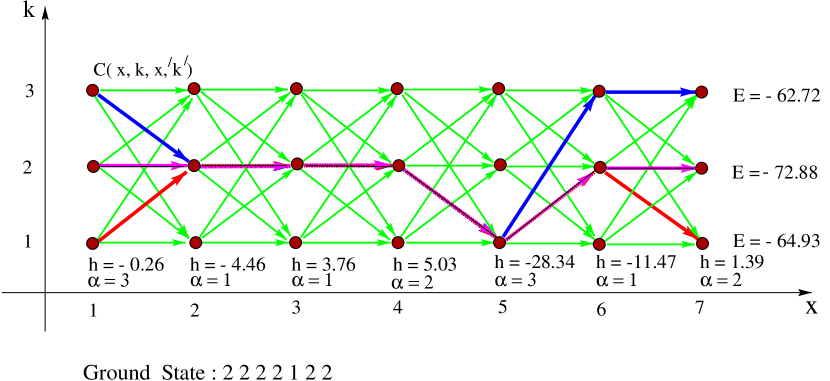
Figure 17: The graph corresponding to the Shortest Path Method for the RFPC problem.

The ground state of $q$-State RFPC can be calculated exactly by mapping onto a shortest path problem on an acyclic graph. The graph $G(L,q)$ corresponding to a $q$-State RF Potts chain of length $L$ consists of ($L$+1)$\times q$ nodes which we consider to be arranged like presented in figure 1 and denoted by ($x,k$) with $x=1,....,L$ and $k=1,....,q$. Each node ($x,k$) is connected to all of its right neighbours, i.e. to all nodes ($x+1,k^{\prime}$) with $k^{\prime}=1,....,q$ by a directed one-way edge with cost

$$c_{(x,x+1,{k},{k}^{\prime})}=-J(q\delta_{\vec{k},\vec{k^{\prime}}}-1)-h_{x+1}(q\delta_{\vec{k},\vec{\alpha}}-1).$$ (32)

Fixing the spin at $x=$ 0 to be in state $k$ the groundstate of RFPC then corresponds to a shortest path from ($1,k$) to ($L,k$) in $G$($L,k$). To apply periodic boundary conditions it is necessary to solve $q$ shortest path problems, one for each of the $q$ (with $(q,q)$ spins at sites $x=$ 1 and $x=L$+1) possible states. One of these shortest paths with minimum energy gives rise to the optimal groundstate.

Since the underlying graph (Fig. 17) is acyclic no cycle, in particular none with negative weight, can occur and Dijkstra’s algorithm for finding the shortest path in a weighted graph can be applied although not all edge weights are positive. The running time of this algorithm is linear both in number $n$ of the nodes and in the number $m$ of the edges, thus the overall complexity to find the groundstate of the RFPC with periodic boundary condition is $\mathcal{O}$($q^{2}L$).

Appendix B

For temperature $T>0$ we generalize the Transfer Matrix Method Crisanti93 for the $q$-States RFPC. The calculation of the partition function ${\mathcal{Z}}_{N}$ can be reduced to the problem of finding the product of $N$ random matrices:

$${\mathcal{Z}}_{N}=\sum_{\{\sigma\}}exp(-\beta{\mathcal{H}}{\sigma})=Tr\left(\prod_{i=1}^{N}{{\bf L}^{(i)}}\right)$$ (33)

where

$${\bf L}^{(i)}_{j,k}=\left[\begin{array}[]{c}\exp[\beta J(q\delta_{\vec{\sigma_{j}},{\vec{\sigma_{k}}}}-1)+\beta h_{i}(q\delta_{\vec{\sigma_{j}},{\vec{\alpha_{i}}}}-1)]\end{array}\right]_{q\times q},$$ (34)

Here ($j,k=1,...,q$).

Using this expression of partition function the expectation value $\langle\sigma_{r}\rangle$ for each spin can be expressed as,

$$\langle\sigma_{r}\rangle=\frac{\sum_{\{\sigma\}}\sigma_{r}exp{(-\beta{\mathcal{H}})}}{{\mathcal{Z}}_{N}}$$ (35)

It is easy to see from Eq. (23) that

$$\langle\sigma_{r}\rangle=\frac{{Tr\left[\left(\prod_{i=1}^{N}{\bf L}^{(i+r-1)}\right){\bf S}\right]}}{Tr\left(\prod_{i=1}^{N}{\bf L}^{(i+r-1)}\right)}$$ (36)

with ${\bf{S}}_{ij}=i.\delta_{ij}$.

The only computational effort consists in calculating the product of $N$ $q\times q$ transfer matrices. Since the elements of ${\bf L}^{(i)}$ become very small for low temperatures, arbitrarily small temperatures can not be considered. However, the admissible temperature interval is sufficient for our investigations.

References

- (1) See e.g. Spin Glasses and Random Fields, ed. A. P. Young, (World Scientific, Singapore, 1997) for a review.
- (2) H. Rieger and A. P. Young, J. Phys. A 26, 5279, (1993); H. Rieger, Phys. Rev. B 52, 6659 (1995).
- (3) J.-C. Anglès d’Auriac and N. Sourlas, Europhys. Lett., 39, 473 (1997); S. Bastea and P. M. Duxbury, Phys Rev. E. 58, 4261 (1998); A. K. Hartmann and U. Nowak, Eur. Phys. J. B 7, 105 (1999); A. A. Middleton and D. S. Fisher, Phys. Rev. B 65, 134411 (2002) and references therein.
- (4) H. Rieger, Frustrated Systems: Ground State Properties via Combinatorial Optimization, Lecture Notes in Physics 501, p.122 (Springer Verlag Heidelberg, 1998).
- (5) M. Alava, P. Duxbury, C. Moukarzel and H. Rieger, Combinatorial optimization and disordered systems, in: “Phase transition and Critical Phenomena” vol. 18 (eds. C. Domb and J. L. Lebowitz), p. 141 (Academic Press, Cambridge, 2000).
- (6) A. K. Hartmann and H. Rieger, Optimization algorithms in physics (Wiley, Berlin 2002)
- (7) G. Schröder, T. Knetter, M. J. Alava and H. Rieger, Eur. Phys. J. B 24, 101 (2001).
- (8) H. Nishimori, Phys. Rev. B 28, 4011 (1983); R. Riera, C.M. Chaves, and R.R. dos Santos, Phys. Rev. B 31, 3093 (1985); J.F. Fontanari, W.K. Theumann, and D.R.C. Dominguez, Phys. Rev. B 39, 7132 (1989).
- (9) For the RF Potts model in more general context, see: D. Blankschtein, Y. Shapir, and A. Aharony, Phys. Rev. B 29, 1263 (1984); K. Eichhorn and K. Binder, J. Phys. Cond. Mat. 8, 5209 (1996).
- (10) R. Bruinsma and G. Aeppli, Phys. Rev. Lett. 50, 1494 (1983).
- (11) David Andelman, Phys. Rev. B 34, 6214 (1986).
- (12) J. Bene and P. Szépfalusy, Phys. Rev. A 37, 1703 (1988).
- (13) For a review on anomalous and Sinai diffusion see J. P. Bouchaud and A. Georges, Phys. Rep. 195, 127(1990).
- (14) Daniel S. Fisher, Pierre Le Doussal, and Cécile Monthus Phys. Rev. E 64, 066107 (2001)
- (15) Y. Imry and S.-K. Ma, Phys. Rev. Lett. 35, 1399 (1975).
- (16) H. Rieger, L. Santen, U. Blasum, M. Diehl, M. Jünger, and G. Rinaldi, J. Phys. A: Math. Gen. 29, 3939 (1996).
- (17) A. J. Bray and M. A. Moore 1985 Heidelberg Colloquium on Glassy Dynamics and Optimization eds. L. van Hemmen and I. Morgenstern (Heidelberg: Springer); 1986 Advances on Phase Transition and Disorder Phenomena eds. G. Busiello and L. Deces (World Scientific, Singapore).
- (18) T. Aspelmeier, A. J. Bray, and M. A. Moore, cond-mat/0207300; P. E. Jönsson, H. Yoshino, and P. Nordblad, Phys. Rev. Lett. 89, 097201, (2002); A. Billoire and E. Marinari, cond-mat/9910352.
- (19) M. Alava and H. Rieger, Phys. Rev. E 58, 4284 (1998).
- (20) N.-N. Pang, Y.-K. Yu and T. Halpin-Healy, Phys. Rev. E 52, 3 (1995).
- (21) J. C. Anglès d’Auriac, M. Preissmann and A. Seb, Math. Comput. Model. 26, 1 (1997).
- (22) A. Crisanti, G. Paladin, A. Vulpiani, Products of Random Matrices in Statistical Physics, Springer Series in Solid-State Sciences 104, (Springer-Verlag, Heidelberg, 1993).