Correlations in the low-temperature phase of the two-dimensional $XY$ model

Abstract

Monte Carlo simulations of the two-dimensional $XY$ model are performed in a square geometry with fixed boundary conditions. Using a conformal mapping it is very easy to deduce the exponent $\eta_{\sigma}(T)$ of the order parameter correlation function at any temperature in the critical phase of the model. The temperature behaviour of $\eta_{\sigma}(T)$ is obtained numerically with a good accuracy up to the Kosterlitz-Thouless transition temperature. At very low temperatures, a good agreement is found with Berezinskii’s harmonic approximation. Surprisingly, we show some evidence that there are no logarithmic corrections to the behaviour of the order parameter density profile (with symmetry breaking surface fields) at the Kosterlitz-Thouless transition temperature.

The two-dimensional classical $XY$ model is very famous in statistical physics, both for fundamental reasons, as describing for example classical Coulomb gas or fluctuating surfaces, and because of its relevance for the description of real systems, e.g. Helium super-fluid films. The model undergoes a standard temperature-driven paramagnetic to ferromagnetic phase transition in $d>2$, characterised e.g. by a power-law divergence of the correlation length near criticality, $\xi\sim|t|^{-\nu}$, (see e.g. Ref. [1]) while it exhibits a rather different behaviour in two dimensions, where the existence of a low-temperature phase with conventional long range order is precluded by the Mermin-Wagner theorem [2]. Indeed there is no spontaneous magnetisation at any nonzero temperature in one or two-dimensional isotropic systems with short range interactions and having a continuous symmetry group, for example $O(n)$ spin models for $n\geq 2$, since order would otherwise be destroyed by spin wave excitations [3]. Such systems can however display a low-temperature phase with topological order and the defect-mediated transition is governed by unbinding of topological defects. At low temperature, the system is partially ordered, apart from the topological defects (vortices in the case of the $2d$ $XY$-model) which appear in pairs, in increasing number with increasing temperature. At the transition temperature, the pairs are broken and the system becomes completely disordered. The low-temperature regime was investigated by Berezinskii [3] in the harmonic approximation and the mechanism of unbinding of vortices was studied by Kosterlitz and Thouless [4, 5] using approximate renormalization group methods. For reviews, see e.g. Refs. [6, 7, 8, 9].

This very peculiar topological transition is characterised by essential singularities when approaching the critical point from the high temperature phase, $\xi\sim{\rm e}^{b_{\xi}t^{-\nu}}$, $\chi\sim{\rm e}^{b_{\chi}t^{-\nu}}$, while in the low-temperature phase, there is a line of critical points and the order parameter correlation function decays algebraically with an exponent $\eta_{\sigma}(T)$ which depends on the temperature. Consider a square lattice with two-components spin variables $\vec{\phi}_{w}=(\cos\theta_{w},\sin\theta_{w})$ with continuous $O(2)$ symmetry, located at the sites $w$ of a lattice $\Lambda$ of linear extent $L$, and interacting through the usual nearest-neighbour interaction

$$-\frac{H}{k_{B}T}=K\sum_{w}\sum_{\mu}\vec{\phi}_{w}\cdot\vec{\phi}_{w+\hat{\mu}}=K\sum_{w}\sum_{\mu}\cos(\theta_{w}-\theta_{w+\hat{\mu}}),$$ (1)

where $\mu$ labels the directions and $\hat{\mu}$ is a unit vector in the $\mu-$direction. The low-temperature or spin-wave behaviour is obtained in the harmonic approximation, after expanding the cosine, which should be justified at sufficiently low temperature where existence of order, at least at short range, is assumed:

$$-\frac{H}{k_{B}T}\simeq-\frac{H_{0}}{k_{B}T}-\frac{1}{2}K\sum_{w}\sum_{\mu}(\theta_{w}-\theta_{w+\hat{\mu}})^{2}.$$ (2)

Within this approximation, the two-point correlator becomes

$$\langle\vec{\phi}_{w_{1}}\cdot\vec{\phi}_{w_{2}}\rangle \simeq Z_{\beta}^{-1}\prod_{w}\int\frac{d\theta_{w}}{2\pi}\cos(\theta_{w_{1}}-\theta_{w_{2}})\times e^{-\frac{1}{2}K\sum_{w}\sum_{\mu}(\theta_{w}-\theta_{w+\hat{\mu}})^{2}}$$ (3)

$$\simeq |w_{1}-w_{2}|^{-1/2\pi K},$$

hence $\eta(T)=T/2\pi$. The low-temperature phase thus has the characteristic features of a critical phase with local scale invariance, i.e. conformal invariance (invariance under rotation, translation and scale transformations, short-range interactions, isotropic scaling). Conformal invariance is known as a powerful framework for the description of two-dimensional critical systems [10]. In the case of the $XY$ model, the central charge is $c=1$ in agreement with the continuous variation of critical exponents in the low-temperature phase. The scaling dimensions $x_{n,m}$ of the primary operators ${\cal O}_{n,m}$ depend on a parameter $\rho$ (called compactification radius),

$$x_{n,m}=\frac{1}{2}(n^{2}/\rho^{2}+m^{2}\rho^{2}).$$ (4)

The spin operator is identified to the conformal operator ${\cal O}_{1,0}$ and the vortex operator to ${\cal O}_{0,1}$ [10]. This is coherent with the picture according to which in the high-temperature phase, the vortices are unbounded and produce the disordering of the system, the vortex chemical potential playing the rôle of a relevant operator. Then vortices and anti-vortices begin to bind, decreasing their relevance when the temperature decreases to become marginal at $T_{\rm KT}$, where the condensation of defects occurs. There, $x_{0,1}$ must be 2 (for the RG eigenvalue $y=d-x_{0,1}$ to vanish), implying that $\rho=2$. Hence at the KT transition, the exponent of the spin-spin correlation function decay takes the value predicted by Kosterlitz and Thouless, $\eta_{\sigma}(T_{\rm KT})=2x_{1,0}=1/4$. The corresponding values in the critical phase below $T_{\rm KT}$ would in principle easily be deduced from equation (4), but the dependence of $\rho$ on the temperature is not known. Unfortunately, not much is known in the intermediate regime between the spin wave approximation at low temperature and the Kosterlitz-Thouless results at the topological transition and in fact the precise determination of the critical behaviour of the two-dimensional $XY$ model in the critical phase remains a challenging problem. Many results were obtained using Monte Carlo simulations (see e.g. Refs. [11, 12, 13, 14, 15, 16]) at $T_{\rm KT}$ or high-temperature series expansions [17], but the analysis was made difficult due to the existence of logarithmic corrections, e.g. $\chi\sim\xi^{2-\eta_{\sigma}}(\ln\xi)^{-2r}$ in the high-temperature regime, or $\langle\vec{\phi}_{w_{1}}\cdot\vec{\phi}_{w_{2}}\rangle\simeq|w_{1}-w_{2}|^{-\eta_{\sigma}}(\ln|w_{1}-w_{2}|)^{\eta_{\sigma}/2}$ at $T_{\rm KT}$ exactly [8] and the value of $\eta_{\sigma}$ at $T_{\rm KT}$ was a bit controversial as shown in table 1 of reference [16]. The resort to large-scale simulations was then needed in order to confirm this picture [15].

In the following, we use a rather different approach which does not require so extensive simulations. Assuming that the low-temperature phase exhibits all the characteristics of a critical phase with conformal symmetry, we simply use the covariance law of $n-$point correlation functions under the mapping of a two-dimensional system confined inside a square onto the half-infinite plane. The scaling dimensions are then obtained through a simple power-law fit where the shape effects are encoded in the conformal mapping. This is the crucial point, since then even very small systems are well adapted to such fits, apart from irrelevant lattice effects. We note that mappings inside a square and various other geometries have been considered already, e.g. the moments of the magnetization [18] and structure factors [19] in the Ising model have been calculated in square systems.

The order parameter correlation function in a square system, $\langle\vec{\phi}_{w_{1}}\cdot\vec{\phi}_{w_{2}}\rangle$, should in principle lead to the determination of critical exponents, but practically, it is not of great help since strong surface effects occur which modify the large-distance power-law behaviour. The correlation function is supposed to obey a scaling form which reproduces the expected power-law behaviour in the thermodynamic limit, for example $\langle\vec{\phi}_{w_{1}}\cdot\vec{\phi}_{w_{2}}\rangle=|w_{1}-w_{2}|^{-\eta_{\sigma}}f_{\rm sq.}(w_{1}/L,w_{2}/L)$, where $f_{\rm sq.}$ encodes shape effects in a very complicated manner. Conformal invariance provides an efficient technique to avoid these shape effects, or at least, enable to include explicitly the shape dependence in the functional expression of the correlators through the conformal covariance transformation under a mapping $w(z)$:

$$\langle\vec{\phi}_{w_{1}}\cdot\vec{\phi}_{w_{2}}\rangle=|w^{\prime}(z_{1})|^{-x_{\sigma}}|w^{\prime}(z_{2})|^{-x_{\sigma}}\langle\vec{\phi}_{z_{1}}\cdot\vec{\phi}_{z_{2}}\rangle$$ (5)

with $\eta_{\sigma}=2x_{\sigma}$. In the semi-infinite geometry $z=x+iy$ (the free surface being defined by the $x$ axis), the two-point correlator is fixed up to an unknown scaling function (apart from some asymptotic limits implied by scaling). Fixing one point $z_{1}$ close to the free surface ($z_{1}=i$) of the half-infinite plane, and leaving the second point $z_{2}$ explore the rest of the geometry, the following behaviour is expected: $\langle\vec{\phi}_{z_{1}}\cdot\vec{\phi}_{z_{2}}\rangle_{\frac{1}{2}\infty}\sim(y_{1}-y_{2})^{-x_{\sigma}}\psi(\omega),$ where the dependence on $\omega={y_{1}y_{2}}/{\mid z_{1}-z_{2}\mid^{2}}$ of the universal scaling function $\psi$ is constrained by the special conformal transformation [20]. In order to get a functional expression of the correlation function inside the square geometry $w$, one simply has to use the mapping $w(z)$ which realizes the conformal transformation of the half-plane $z=x+iy$ ($0\leq y<\infty$) inside a square $w=u+iv$ of size $L\times L$ ($-L/2\leq u\leq L/2$, $0\leq v\leq L$) with free boundary conditions along the four edges. This is realized by a Schwarz-Christoffel transformation [21]

$$w(z)={L\over 2{\rm K}}{\rm F}(z,k),\quad z={\rm sn}\left({2{\rm K}w\over L}\right).$$ (6)

Here, $F(z,k)$ is the elliptic integral of the first kind, ${\rm sn}\ \!(2{\rm K}w/L)$ the Jacobian elliptic sine, ${\rm K}=K(k)$ the complete elliptic integral of the first kind, and the modulus $k$ depends on the aspect ratio of $\Lambda$ and is here solution of $K(k)/K(\sqrt{1-k^{2}})=\frac{1}{2}$. Using the mapping (6), the local rescaling factor in equation (5) is obtained, $w^{\prime}(z)=\frac{L}{2{\rm K}}[(1-z^{2})(1-k^{2}z^{2})]^{-1/2}$, and inside the square, keeping $w_{1}$ fixed, the two-point correlation function becomes (see e.g. Ref. [22])

$$\langle\vec{\phi}_{w_{1}}\cdot\vec{\phi}_{w}\rangle_{\rm sq.}\sim{\underbrace{\left(\Im[z]./\sqrt{|1-z^{2}|.|1-k^{2}z^{2}|}\right)}_{\kappa(w)}}^{-x_{\sigma}}\psi(\omega),$$ (7)

with $z(w)$ given by equation (6). This expression is correct up to a constant amplitude determined by $\kappa(w_{1})$ which is kept fixed, but the function $\psi(\omega)$ is still varying with the location of the second point, $w$. In order to cancel the rôle of the unknown scaling function, it is more convenient to work with a density profile $m(w)$ in the presence of symmetry breaking surface fields $\vec{h}_{\partial\Lambda}$ on the boundary $\partial\Lambda$ of the lattice $\Lambda$. This one-point correlator scales in the half-infinite geometry $m(z)=\langle\vec{\phi}_{z}\cdot\vec{h}_{\partial\Lambda(z)}\rangle_{\frac{1}{2}\infty}={\rm const\times}y^{-x_{\sigma}}$and it maps onto

$$m(w)=\langle\vec{\phi}_{w}\cdot\vec{h}_{\partial\Lambda(w)}\rangle_{\rm sq.}={\rm const\times}[\kappa(w)]^{-x_{\sigma}}$$ (8)

where the function $\kappa(w)$ defined in equation (7) again comes from the mapping.

The application of the simple power-law in equation (8) requires a relatively precise numerical determination of the order parameter profile of the $2d$ $XY$ model confined inside a square with fixed boundary conditions playing the rôle of ordering surface fields $\vec{h}_{\partial\Lambda(w)}$. In practice, no magnetic field is applied, but the symmetry is broken by keeping the boundary spins of the square fixed, e.g. $\vec{\phi}_{w}=(1,0),\forall w\in\partial\Lambda$ during the Monte Carlo simulations (in principle no update of these spins is performed). In the low-temperature phase, local Metropolis updates of single spins are known to suffer from the critical slowing down, since the system contains arbitrarily large clusters in which the spin orientations are strongly correlated. Statistically independent configurations can be obtained by local iteration rules only after a long dynamical evolution which needs a huge number of MC steps, sometimes beyond nowadays computers capability. The resort to cluster update algorithms (like Wolff algorithm) is more convenient. The central idea of cluster algorithms is the identification of clusters of sites using a bond percolation process connected to the spin configuration. The spins of the clusters are then independently updated. A cluster algorithm is particularly efficient if the percolation threshold coincides with the transition point of the spin model, which guarantees that clusters of all sizes will be updated in a single MC sweep. The percolation process associated to Ising or Potts models is the random graph model of the Fortuin-Kasteleyn representation and its threshold is known to coincide with the critical point of the spin model. For the $XY$ model, the bonds are introduced in the Wolff algorithm through the definition of Ising variables defined by the sign of the projection of the spin variables along some random direction. The percolation threshold for these bonds coincides with the Kosterlitz-Thouless point [23], which guarantees the efficiency of the Wolff cluster updating scheme [13] at $T_{\rm KT}$. In the low-temperature phase, this algorithm could be less efficient, but nevertheless preferable to a local updating. When one uses particular boundary conditions, with fixed spins along some surface as required here, the Wolff algorithm should become less efficient, since close to criticality the unique cluster will often reach the boundary and no update is made in this case. To prevent this, we use the symmetry properties of the Hamiltonian (1). Even when the cluster reaches the fixed boundaries $\partial\Lambda(w)$, it is updated, and the order parameter profile is then measured with respect to the common new direction of the boundary spins, $m(w)=\langle\vec{\phi}_{w}\cdot\vec{\phi}_{\partial\Lambda}\rangle_{\rm sq.}$. The new configuration reached would thus correspond - after a global rotation of all the spins of the system to re-align the boundary spins in the $(1,0)$ direction - to a a new configuration of equal total energy and thus the same statistical weight as the one actually produced. This technique eventually leads to a new update at each iteration: when the cluster does not touch the boundaries, all the spins belonging to the cluster are updated, and in the other case the situation becomes equivalent to an update of all the spins but those inside the cluster. At a percolation threshold, interior and exterior of a percolating cluster are both large and intricated and the algorithm has short time correlations. After averaging over the ‘production sweeps’, one gets a characteristic smooth profile.

  

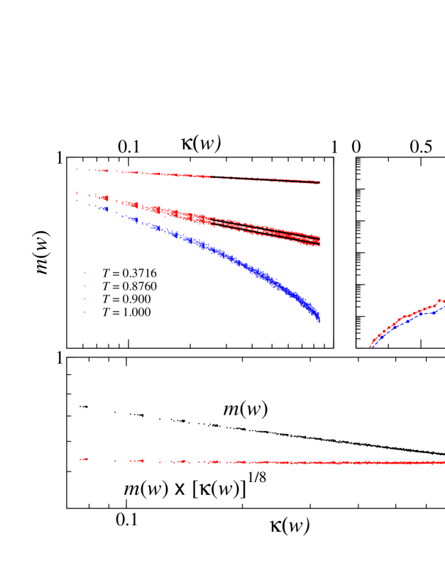
Fig. 1.–: Monte Carlo simulations of the $2d$ $XY$ model inside a square $100\times 100$ spins ($10^{6}$ MCS/spin after cancellation of $10^{6}$ for thermalization, cluster update algorithm). Top: on the left, the figure shows the rescaled order parameter density against the rescaled distance on a log-log scale at different temperatures below the Kosterlitz-Thouless transition temperature and slightly above. On the right, we show a plot of the $\chi^{2}$ per d.o.f. of the power-law fits as a function of the temperature for $L=48$ and $100$. The sharp change of behaviour is a signature of the location of the Kosterlitz-Thouless transition, above which the functional expression (8) of the density profile is no longer correct. Bottom: plot of the density profile $m(w)$ with symmetry breaking surface field and of the rescaled quantity $m(w)\times[\kappa(w)]^{1/8}$ vs $\kappa(w)$ on a log-log scale (exactly at the Kosterlitz-Thouless transition temperature). The rescaled profile remains constant with a very good accuracy, indicating the absence of logarithmic correction for this quantity.

  

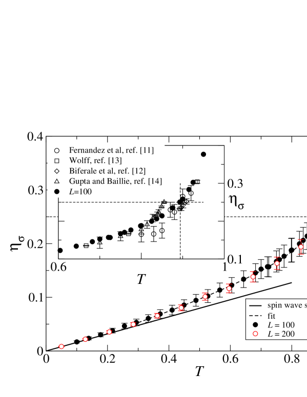
Fig. 2.–: Correlation decay exponent of the $2d$ $XY$ model as a function of the temperature. The insert shows a comparison with other results (in the vicinity of the KT point) found in the literature.

A log-log plot of $m(w)$ with respect to the reduced variable $\kappa(w)$ is shown in figure 1 at two different temperatures below $T_{\rm KT}\simeq 0.893(1)$ (the value of $T_{\rm KT}$ is taken according to reference [14]), roughly at $T_{\rm KT}$, and one temperature slightly above. The first message of the plot is the confirmation of the functional form of equation (8). One indeed observes a very good data collapse of the $L^{2}$ points onto a single power-law master curve (a straight line on this scale). The next information is the rough confirmation of the value of the critical temperature, since above $T_{\rm KT}$, the master curve is no longer a straight line, indicating that the corresponding decay in the half-infinite geometry differs from a power-law as it should in the high-temperature phase. One should nevertheless mention that this is not a technique adapted to a precise determination of $T_{\rm KT}$, since at $T=0.9$ for example, the master curve is hardly distinguishable from a straight line. One can for example compute the $\chi^{2}$ per d.o.f. as a function of temperature. It has a very small value, indicating the high quality of the fit, in the low-temperature phase and then increases significantly above $T_{\rm KT}$ when the behaviour of the density profile is no longer algebraic. The change of behaviour in the curve gives an approximate location of the Kosterlitz-Thouless transition temperature, and the larger the system size, the better this estimate. This is illustrated in figure 1.

It is tempting to study the rôle of logarithmic corrections exactly at the Kosterlitz-Thouless point. For that purpose, we produce data at a temperature $T=T_{\rm KT}$ and, assuming that logarithmic corrections should affect the density profile with symmetry breaking surface field in the half-infinite geometry, we make a plot of $m(w)\times[\kappa(w)]^{1/8}$ vs $\kappa(w)$. Surprisingly, this leads very accurately to a constant, as shown in figure 1. This is a clear evidence that the order parameter profile with fixed boundary conditions displays a pure algebraic decay at the Kosterlitz-Thouless transition point. The decay exponent, if not fixed, but determined numerically, leads to a quite good result (for example for a size $L=100$, we get $\eta_{\sigma}(T_{\rm KT})=0.250(28)$).

It is thus possible to obtain the scaling dimension $x_{\sigma}(T)$ or the two-point correlation function exponent $\eta_{\sigma}(T)=2x_{\sigma}(T)$, in the whole critical region $T\leq T_{\rm KT}$ as shown in figure 2. The most interesting result obtained here is perhaps the fact that the values of the exponent $\eta$ are very easy to obtain, in spite of the reputed difficulty of this problem from MC studies. For example the results obtained with a system of size as small as $48\times 48$ are already very satisfying, and to get 10 values of $T$ ($10^{5}$ MCS/spin for thermalization $+10^{6}$ MCS/spin for computation) corresponds to a quite reasonable amount of 11 hours of CPU time on a standard PC with 733 MHz processor (the algorithm is more efficient at $T_{\rm KT}$ than below) . For the largest size considered here, $L=200$, a simulation at the Kosterlitz-Thouless temperature needs 18 hours ($10^{6}+10^{6}$ MCS/spin) which is also very fast compared to today’s standard extensive simulations where the natural time unit is the CPU-year. We mention here that we do not reach the accuracy of the very precise numerical determination of the magnetic scaling dimension (using transfer matrix techniques) by Blöte and Nienhuis [24].

Once the values of these scaling dimensions are known, we can deduce numerically the temperature-behaviour of the compactification parameter $\rho$, and thus perhaps conjecture the numerical values of other scaling dimensions associated to different operators. Up to the authors knowledge, such an approach has not yet been done and it could be promising for a better understanding of the critical phase of the Kosterlitz-Thouless transitions. From the numerical data, $\eta_{\sigma}(T)$ is easily expanded close to the KT point $T\to T_{\rm KT}^{-}$, showing a leading square root behaviour [5],

$$\eta_{\sigma}\sim\frac{1}{4}-0.231(T_{\rm KT}-T)^{1/2}-0.050(T_{\rm KT}-T)^{3/2},$$ (9)

shown as a fit in figure 2 and from which it is easy to write the first terms of an expansion of the compactification radius, $\rho\simeq 2[1+0.462(T_{\rm KT}-T)^{1/2}+0.320(T_{\rm KT}-T)+\dots]$ when $T\to T_{\rm KT}^{-}$. This leads in principle to an approximate value of the other scaling dimensions through equation 4.

***

BB would like to thank Christophe Chatelain for stimulating discussions and Dragi Karevski for a critical reading of the manuscript.

References

- [1] M. Hasenbusch and T. Török, J. Phys. A 32, 6361 (1999).
- [2] N.D. Mermin and H. Wagner, Phys. Rev. Lett. 22, 1133 (1966).
- [3] V.L. Berezinskii, Sov. Phys. JETP 32, 493 (1971).
- [4] J.M. Kosterlitz and D.J. Thouless, J. Phys. C 6, 1181 (1973).
- [5] J.M. Kosterlitz, J. Phys. C 7, 1046 (1974).
- [6] J.M. Kosterlitz and D.J. Thouless, Prog. Low Temp. Phys 78, 371 (1978).
- [7] D.R. Nelson, in Phase Transitions and Critical Phenomena, ed. by C. Domb and J.L. Lebowitz, Academic Press, London 1983, p. 1.
- [8] C. Itzykson and J.M. Drouffe, Statistical field theory, Cambridge University Press, Cambridge 1989, vol. 1.
- [9] Z. Gulácsi and M. Gulácsi, Adv. Phys. 47, 1 (1998).
- [10] M. Henkel, Conformal Invariance and Critical Phenomena, Springer, Heidelberg 1999.
- [11] J.F. Fernández, M.F. Ferreira and J. Stankiewicz, Phys. Rev. B 34, 292 (1986).
- [12] L. Bifferale and R. Petronzio, Nucl. Phys. B 328, 677 (1989).
- [13] U. Wolff, Nucl. Phys. B 322, 759 (1989).
- [14] R. Gupta and C.F. Baillie, Phys. Rev. B 45, 2883 (1992).
- [15] W. Janke, Phys. Rev. B 55, 3580 (1997).
- [16] R. Kenna and A.C. Irving, Nucl. Phys. B 485 [FS], 583 (1997).
- [17] P. Butera and M. Comi, Phys. Rev. B 50, 3052 (1994).
- [18] T.W. Burkhardt and B. Derrida, Phys. Rev. B 32, 7273 (1985).
- [19] P. Kleban, G. Akinci, R. Hemtschke and K.R. Brownstein, J. Phys. A 19, 437 (1986).
- [20] J. L. Cardy, Nucl. Phys. B 240 [FS12], 514 (1984).
- [21] M. Lavrentiev and B. Chabat, Méthodes de la théorie des fonctions d’une variable complexe, Mir, Moscou 1972, Chap. VII.
- [22] C. Chatelain and B. Berche, Phys. Rev. E 60, 3853 (1999).
- [23] I. Dukovski, J. Machta and L.V. Chayes, Phys. Rev. E 65, 026702 (2002).
- [24] H.W.J. Blöte and B. Nienhuis, J. Phys. A 22, 1415 (1989).