Resistance of a domain wall in the quasiclassical approach

Abstract

Starting from a simple microscopic model, we have derived a kinetic equation for the matrix distribution function. We employed this equation to calculate the conductance $G$ in a mesoscopic F’/F/F’ structure with a domain wall (DW). In the limit of a small exchange energy $J$ and an abrupt DW, the conductance of the structure is equal to $G_{2d}=4\sigma_{\uparrow}\sigma_{\downarrow}/(\sigma_{\uparrow}+\sigma_{\downarrow})L$. Assuming that the scattering times for electrons with up and down spins are close to each other we show that the account for a finite width of the DW leads to an increase in this conductance. We have also calculated the spatial distribution of the electric field in the F wire. In the opposite limit of large $J$ (adiabatic variation of the magnetization in the DW) the conductance coincides in the main approximation with the conductance of a single domain structure $G_{1d}=(\sigma_{\uparrow}+\sigma_{\downarrow})/L$. The account for rotation of the magnetization in the DW leads to a negative correction to this conductance. Our results differ from the results in papers published earlier.

I Introduction

In ferromagnetic metals not only the charge of the electron but also the spin plays an important role in transport phenomena. A famous example is the observation of the giant magnetoresistance in magnetic multilayers, which can be explained in terms of a spin dependent electronic scattering.

The presence of a domain wall (DW) in a ferromagnet can also change transport properties and this has been observed in a number of experiments. At the first glance, experimental data seems to contradict to each other. In Refs. [1, 2, 3, 4] it was found that the resistance of ferromagnetic wires and films decreases when increasing the external magnetic field, whereas in Refs. [5, 6] the resistance at zero magnetic field was found to be smaller than the one measured at high magnetic fields.

In order to give a quantitative description of these experiments not only the DW contribution to the magnetoresistance (MR) should be taken into account but also other mechanisms, as the anisotropic magnetoresistance, which arises due to the spin-orbit scattering [7, 8, 9], size effects and the Lorentz contribution inside the domains. The main experimental difficulty in determining the DW contribution is to exclude the other effects. For example in Ref.[1] the negative MR observed in Co films was interpreted in terms of DW scattering. However in Ref.[3] it was claimed that the predominant contributions to the observed magnetoresistance of Co films can be explained by a specific micromagnetic structure, which consists of stripe-domains with magnetization out-of-the-film plane. In addition, the films show closure caps at the surfaces with magnetization in plane and parallel to the current. Thus, the resistivity anisotropy might play a fundamental role.

Understanding the details of these experiments is an interesting task. However, before taking into account all material specific characteristics of the experiments one should be able to describe general properties of electron scattering on domain walls. In this paper, we do not try to give an explanation of all these experiments, but solve an idealized model that may capture the most general features of transport in the presence of a DW. We calculate the resistance of a ferromagnetic wire with a DW and restrict ourself to the case when the magnetization of the ferromagnetic structure remains always perpendicular to the current. This assumption simplifies the situation because in this case anisotropic effects do not contribute to the change of the resistance.

The DW contribution to the conductance has been considered in several theoretical works, in which different approaches have been used. For example in Refs. [10, 11] quantum effects (weak localization) were taken into account. It was shown that a DW contributes to the decoherence of electrons leading to a decrease of the resistance. These effects may be important at very low temperatures when localization effects start playing a noticeable role.

At higher temperatures the weak localization effects are not important and one may try to describe the magnetoresistance in terms of classical motion. In recent works, Refs. [12, 13], an increase of the resistance due to a DW was predicted on the basis of a Boltzmann equation. However, the collision term describing scattering of conduction electrons on impurities was introduced phenomenologically.

The classical DW resistance was calculated also in Ref. [14]. In that work, it was shown that the DW resistance could be both negative and positive depending on the difference between the momentum relaxation times $\tau_{\uparrow,\downarrow}$ for the different spin directions. However, the classical Drude expression for the resistivity was used, in which the relaxation times $\tau_{\uparrow,\downarrow}$ were introduced again as phenomenological parameters.  In Refs.[15, 16] the resistance of a DW located in a point contact was calculated.

The purpose of this paper is to derive a proper kinetic equation for the distribution function from a microscopic model and to calculate the DW resistance on its basis. We employ a standard approach based on microscopic equations for the quasiclassical Green’s functions in the Keldysh technique. Assuming that the impurity scattering potential $u_{s}$ is spin dependent, we derive the kinetic equation for the matrix (in the Nambu and spin space) distribution function. As a result we come to the kinetic equation for the ditribution function $f$ that is a $2\times 2$ matrix in the spin space. The impurity scattering potential which enters the collision integral is also a matrix and this makes the equation considerably more complicated than the standard one that could be written for a spin independent scattering.

Throughout this article we assume that the magnetization remains always perpendicular to the current. First we solve the derived kinetic equation in two simplest cases: a single domain and two domain structure with an abrupt DW (i.e. the width of the DW equals zero). In the case of a finite DW width we solve the kinetic equation assuming the potentials $u_{\uparrow}$ and $u_{\downarrow}$ do not differ much from each other. Even in this limit, it is hard to obtain analytical formulae for an arbitrary width of the DW. Two different limiting cases naturally arise and this allows us to obtain a solution for the distribution function. The first limit corresponds to a sharp DW (to a small exchange energy $J$ ). The second limit corresponds to a smooth DW ( to a large $J$ ). We note that only the second limit was analyzed in Refs. [12, 13, 17]. As in Refs. [12, 13, 17] we obtain that the DW increases the resistance of the system. However our formulae for the contribution of the DW to the resistance differ essentially from those presented in Refs. [12, 13, 17].

The paper is organized in the following way. In the next section we introduce the model and derive the kinetic equation for the distribution function in a ferromagnetic wire  neglecting quantum effects. We start from the microscopic Hamiltonian (2)  with different scattering rates at impurities for spin-up and spin down-electrons. In the subsequent sections we  calculate the conductance of the system in the diffusive  limit. In section III A we consider the case of a sharp DW when $J\ll D/w^{2},$ where $D$ is the diffusion coefficient, $w$ is the width of the DW and $J$ is the exchange field acting on the electron spin. In section III B we calculate the conductance of a “slowly” varying DW, i. e. we consider the case $D/w^{2}\ll J$. It turns out that in the first case the conductance is always smaller than in the adiabatic case. In the last section we summarize our results.

II Kinetic Equation

In this section we derive the kinetic equation for the matrix distribution function $\hat{f}$ starting from equations for the quasiclassical Green functions. The function $\hat{f}$ is a $2\times 2$ matrix in the spin space. We assume that the impurity scattering rate depends on the spin directions but, for simplicity, we neglect such spin-flip processes as the spin-orbit interaction or the scattering by magnetic impurities. So, in our model each impurity scattering vertex is a matrix that does not commute with $\hat{f}$ and therefore the elastic collision integral has a nontrivial form. This fact has been ignored in Refs. [12, 17], where the collision integral was written phenomenologically.

Using the derived kinetic equation we calculate the conductance of a mesoscopic structure which consists of two reservoirs and a ferromagnetic wire (or film) connecting the reservoirs (see Fig. 1). A domain wall is assumed to be present in the ferromagnet. We consider the diffusive limit, which means that the mean free path is the shortest length (apart from the Fermi wave length) in the problem. We solve the kinetic equation assuming the smallness of the parameter $\beta$, defined as

$$\beta=\frac{\sigma_{\uparrow}-\sigma_{\downarrow}}{\sigma_{\uparrow}+\sigma_{\downarrow}}$$ (1)

where $\sigma_{\uparrow,\downarrow}$ are conductivities for different spin directions. A precise relation between the conductivities $\sigma_{\uparrow,\downarrow}$, as well as the diffusion coefficients $D_{\downarrow,\uparrow}$, the corresponding scattering rates will become clear below.

The assumption $\beta\ll 1$ is valid for ferromagnets with the exchange energy $J$ much smaller than the Fermi energy. We will consider two limiting cases: a) $J<<D_{\uparrow,\downarrow}/w^{2}$ and b) $J>>D_{\uparrow,\downarrow}/w^{2}$, where $D_{\uparrow,\downarrow}$ is the diffusion coefficient for electrons with up and down spins, $w$ is the width of the DW. The case a) corresponds to a sharp DW. The conductance in this case is smaller than the conductance of the structure without the domain wall. A finite width of the domain wall leads to a positive correction to the conductance. The second case corresponds to a smooth (compared to the magnetic length $\sqrt{D/J}$ ) DW. In the limit of a large $w$ the conductance of the structure is close to that of a structure without a DW. With decreasing the width of the DW, the conductance of the structure decreases. Our results significantly differ significantly from the results obtained in other works, where either the collision term was oversimplified [12, 17], or the kinetic equation was not treated in a correct way [13].

We choose the Hamiltonian of the ferromagnet in a simple standard form

$$H=\sum_{s,s^{\prime}}\int dr\{\psi_{s}^{+}(r)[-\nabla^{2}/2m+eV(r)-J{\bf n}\cdot{\bf\hat{\sigma}}]\psi_{s^{\prime}}(r)\}+H_{imp}\;.$$ (2)

where $V(r)$ is a smoothly varying (over the wave length $\lambda_{F}$) electric potential, $J$ is the exchange energy, ${\bf n}$ is the unit vector directed along the magnetization orientation. The term $H_{imp}(r)$ describes the interaction of electrons with impurities and we assume that it depends on the spin direction. The origin of this dependence can be either the band structure or the intrinsec spin dependence of the impurity scattering potential [12]. If the magnetization is aligned along the z-axis, this interaction can be written as

$$H_{imp}=\sum_{i}\int dr\{\psi_{\uparrow}^{+}(r)u_{\uparrow}(r-r_{i})\psi_{\uparrow}(r)+\psi_{\downarrow}^{+}(r)u_{\downarrow}(r-r_{i})\psi_{\downarrow}(r)\}\;.$$ (3)

As in Ref.[18], we introduce new operators

$$\psi_{n,s}=\left\{\begin{array}[]{c}\psi_{s},n=1\\ \psi_{\overline{s}}^{+},n=2\end{array}\right.\;.$$ (4)

In terms of the operators $\psi_{n,s}$ and in the case of an arbitrary angle $\alpha$ between the magnetization vector and the $z$-axis the Hamiltonian (3) can be written as

$$\begin{array}[]{lcl}H_{imp}&=&\sum_{i,n,s}\int dr\psi_{n,s}^{+}(r)\{\hat{\tau}_{3}\otimes\hat{\sigma}_{0}u_{+}(r-r_{i})+(\hat{\tau}_{0}\otimes\hat{\sigma}_{3}\cos\alpha+\hat{\tau}_{3}\otimes\hat{\sigma}_{2}\sin\alpha)u_{-}(r-r_{i}).\}\psi_{n,s}(r)\}\\ &=&\sum_{i,n,s}\int dr\psi_{n,s}^{+}(r)u_{+}\hat{\tau}_{3}\{1+\lambda\check{n}\}\psi_{n,s}\;,\end{array}$$ (5)

where $u_{\pm}=(u_{\uparrow}\pm u_{\downarrow})/2$, $\lambda=u_{-}/u_{+}$ and the matrix $\check{n}$ is defined as $\check{n}=\hat{\tau}_{3}\otimes\hat{\sigma}_{3}\exp[-i\alpha\hat{\tau}_{3}\otimes\hat{\sigma}_{1}]$.

Introducing the operators $\psi_{n,s}$, Eq. (4), leads to an increase of the size of matrix Green functions written below. One has to deal not only with spin space but also with the Nambu one. Actually, this is not necessary if one consideres non-superconducting metals only. However, this extension of the size would become important if the metal wire we consider were in contact with a superconductor. Although we do not consider any superconductivity in the present work, we keep at the moment the Nambu space explicitly having in mind a possible generalization for the superconductivity.

Now we define the Green functions in the Keldysh technique

$$G_{nn^{\prime}}^{ss^{\prime}}(t_{i},t_{k}^{\prime})=(1/i)<T_{C}(\psi_{n,s}(t_{i})\psi_{n^{\prime}s^{\prime}}^{+}(t_{k}^{\prime}))>\;.$$ (6)

where $T_{C}$ means the time ordering along the Keldysh contour $C$. In a standard way we define the retarded (advanced) $G^{R(A)}$ and Keldysh Green function $G$ as well as a matrix ${\bf G}$ composed of the matrices $G^{R(A)}$ and $G$ (see e. g. Ref.[19]). One can obtain an equation for the matrix ${\bf G}$ in the usual way by summing the ladder diagrams in the cross technique [21] (we neglect all crossed diagrams). This equation has the form

$$(i\partial_{t}-H-{\bf\Sigma_{imp}}){\bf G}=1\;$$ (7)

where $H=[-(1/2m)\nabla^{2}+V(t)]\hat{\tau}_{3}\otimes\hat{\sigma}_{0}-J\hat{\tau}_{3}\mbox{$\check{n}$}$, and the self-energy term ${\bf\Sigma_{imp}}$ is given by

$${\bf\Sigma_{imp}}=n_{imp}\check{u}<{\bf G}>\check{u}\;.$$ (8)

Here $\check{u}=u_{+}(1+\lambda\check{n})$, $<{\bf G}>=\nu\int d\xi_{p}\int d\Omega/4\pi\cdot{\bf G}$ and $n_{imp}$ is the concentration of impurities. In the quasiclassical approach the density of states $\nu$ is written in the main approximation with respect to the parameter $J/\epsilon_{F}$, where $\epsilon_{F}$ is the Fermi energy. In this case $\nu$ is the same for both spin-up and spin-down electrons. Notice that the r.h.s of Eq. (8) is a product of matrices, which in a general case do not commute.

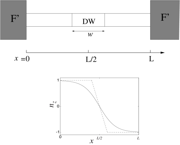
FIG. 1.: Upper Figure: The geometry considered in this article. The domain wall (DW) is situated in the middle of the ferromagnetic wire. Lower Figure: The $z$-component ($n_{z}(x)$) of the magnetization in the F-wire. The solid line corresponds to a Bloch-like wall as calculated by Landau and Lifshitz. The dashed line corresponds to a linear DW

In order to obtain an equation for the quasiclassical Green functions, we follow the standard way (see for example [19] ): we write the equation conjugate to Eq. (7), multiply both equations by $\hat{\tau}_{3}$ and subtract from each other. Then, we integrate the final equation over the variable $\xi_{p}=v_{F}(p-p_{F})$ and obtain

$$\hat{\tau}_{3}\partial_{t}{\bf g}+\partial_{t}{\bf g}\hat{\tau}_{3}+i(eV(t){\bf g}-{\bf g}eV(t))+(v_{F}\nabla){\bf g}+iJ[\mbox{$\check{n}$},{\bf g}]=-(1/2\tau)(\mbox{$\check{m}$}<{\bf g}>\mbox{$\check{m}$}{\bf g}-{\bf g}\mbox{$\check{m}$}<{\bf g}>\mbox{$\check{m}$})\;.$$ (9)

We have introduced the quasiclassical Green function in the usual way

$${\bf g}=(i/\pi)\hat{\tau}_{3}\int d\xi_{p}{\bf G}$$ (10)

The matrix $\check{m}$ is equal to $\mbox{$\check{m}$}=1+\lambda\mbox{$\check{n}$}$ and $\tau^{-1}=\nu n_{imp}|u_{+}|^{2}$ is the mean momentum relaxation rate. The elements of the matrix ${\bf g}$ are $\mbox{$\check{g}$}^{R(A)}$ and $\check{g}$

$${\bf g}=\left(\begin{array}[]{cc}\mbox{$\check{g}$}^{R}&\mbox{$\check{g}$}\\ 0&\mbox{$\check{g}$}^{A}\end{array}\right)$$ (11)

Eq.(9) is valid in a rather general case. In particular, it can be employed in the case of a superconductor-ferromagnet structure when the superconducting condensate penetrates into the ferromagnet. We use Eq.(9) for a normal case, i.e. for F/S structures when one can neglect the penetration of the condensate into the ferromagnet F or for F/F’ structures. In order to obtain the kinetic equation for the distribution function in the normal case, we represent the Keldysh component in the usual form [19]

$$\mbox{$\check{g}$}=\mbox{$\check{g}$}^{R}\cdot\mbox{$\check{f}$}-\mbox{$\check{f}$}\cdot\mbox{$\check{g}$}^{A}$$ (12)

where $\mbox{$\check{g}$}^{R(A)}=\pm\hat{\tau}_{3}\otimes\hat{\sigma}_{0}$ and $\check{f}$ is a 4$\times$4 matrix, whose elements are the components of the distribution function in the Nambu and spin space. This matrix can be represented in the form

$$\mbox{$\check{f}$}=\mbox{$\hat{f}$}_{0}\hat{\tau}_{0}+\mbox{$\hat{f}$}_{3}\hat{\tau}_{3}\;.$$ (13)

The components $\mbox{$\hat{f}$}_{0}$ and $\mbox{$\hat{f}$}_{3}$ are matrices in spin space. In the absence of spin-dependent interactions they are diagonal and related to the distribution functions for electrons $n$ and holes $p$ as follows: $\mbox{$\hat{f}$}_{0}=(1-(n_{s}+p_{\overline{s}}))\cdot\hat{\sigma}_{0}$; $\mbox{$\hat{f}$}_{3}=-(n_{s}-p_{\overline{s}})\cdot\hat{\sigma}_{0}.$ Taking into account Eqs.(10-13), one can easily get from Eq.(9) the kinetic equation for the matrix distribution function

$$\hat{\tau}_{3}(v_{F}\nabla)\mbox{$\check{f}$}+iJ\hat{\tau}_{3}\left[\mbox{$\check{n}$},\mbox{$\check{f}$}\right]=-(1/2\tau)\left[\mbox{$\check{m}$}^{2}\mbox{$\check{f}$}+\mbox{$\check{f}$}\mbox{$\check{m}$}^{2}-2\mbox{$\check{m}$}<\mbox{$\check{f}$}>\mbox{$\check{m}$}\right]\;.$$ (14)

According to all previous definitions we can write

$$\tau_{\uparrow,\downarrow}=\frac{\tau}{(1\pm\lambda)^{2}},$$ (15)

and hence define $\sigma_{\uparrow,\downarrow}$ and $D_{\uparrow,\downarrow}$ without using any phenomenological approach.  In our model the conductivities $\sigma_{\uparrow,\downarrow}$  are equal to: $\sigma_{\uparrow,\downarrow}=e^{2}\nu D_{\uparrow,\downarrow}=e^{2}\nu D(1\pm\lambda)^{-2},$  where $D=v^{2}\tau/3$.  Note that in the absence of superconductivity the distribution function has diagonal in the Nambu- space, and therefore one can take the component (1,1) of Eq. (14) and obtain

$$(v_{F}\nabla)\mbox{$\hat{f}$}+iJ\left[\mbox{$\hat{n}$},\mbox{$\hat{f}$}\right]=-(1/2\tau)\left[\mbox{$\hat{m}$}^{2}\mbox{$\hat{f}$}+\mbox{$\hat{f}$}\mbox{$\hat{m}$}^{2}-2\mbox{$\hat{m}$}<\mbox{$\hat{f}$}>\mbox{$\hat{m}$}\right]\;,$$ (16)

where all matrices are now $2\times 2$ matrices in the spin space. In particular, $\mbox{$\hat{m}$}=1+\lambda\mbox{$\hat{n}$}$ and $\mbox{$\hat{n}$}=\hat{\sigma}_{3}\exp[-i\alpha\hat{\sigma}_{1}]$. Note that the left-hand side of Eq. (16) coincides with the left-hand side of the well known kinetic equation derived for a magnetic material (see for example Ref. [20], where the kinetic equation is presented for a dynamic case in the absence of scattering by impurities). The solution $\hat{f}$ of this equation coincides with the component (1,1) of the distribution function $\check{f}$, which satisfies Eq. (14). Since in this article normal materials (no superconductors) are considered, we will analyze Eq. (16). One can exclude the spatial dependence of the matrices $\hat{n}$ and $\hat{m}$ performing an unitary transformation defined by

$\displaystyle\hat{f}=\hat{U}\cdot\hat{\tilde{f}}\cdot\hat{U}^{+},\;\;\hat{U}=\hat{\sigma}_{0}\cos\alpha/2+i\hat{\sigma}_{1}\sin\alpha/2\;.$

In this case one obtains an equation for the distribution function $\hat{\tilde{f}}$

$$(v_{F}\nabla)\mbox{$\hat{\tilde{f}}$}+i(v_{F}/2)\alpha^{\prime}(x)\left[\hat{\sigma}_{1},\mbox{$\hat{\tilde{f}}$}\right]+iJ\left[\mbox{$\hat{\sigma}_{3}$},\mbox{$\hat{\tilde{f}}$}\right]=-(1/\tau)\left[\mbox{$\hat{\tilde{f}}$}-<\mbox{$\hat{\tilde{f}}$}>+\lambda\left[\hat{\sigma}_{3},\mbox{$\hat{\tilde{f}}$}-<\mbox{$\hat{\tilde{f}}$}>\right]+\lambda^{2}\left(\mbox{$\hat{\tilde{f}}$}-\hat{\sigma}_{3}<\mbox{$\hat{\tilde{f}}$}>\hat{\sigma}_{3}\right)\right]\;.$$ (17)

The left-hand side of this equation differs from the one derived in Ref.[13]. In the latter there is an additional term of the form $(\alpha^{\prime}(x)/4m)[\hat{\sigma}_{1},(\partial F/\partial x)]_{+}$ which, as we have shown, does not appear in the quasiclassical approach. Moreover, due to this term the kinetic equation of Ref. [13] violates the particle number conservation and therefore leads to wrong results. Notice also, that the collision term ( right-hand side of Eq. (17) ) after the unitary rotation may not be diagonal in spin space. This fact was ignored in Refs. [12, 17]. We will see in the next sections that in the case $(D/w^{2})\ll J$, it is convenient to work with Eq.(17), while in the opposite case it is easier to solve the kinetic equation in its original form Eq. (16). We assume that the system is diffusive (this implies the condition $J\tau<<1$) . In this case one can expand the distribution function $\hat{f}$   in spherical harmonics and consider only the first two of them

$$\mbox{$\hat{f}$}=\mbox{$\hat{s}$}+\mu\mbox{$\hat{a}$}\;,$$ (18)

where $\mu=\cos\theta$  and $\theta$  is the angle between $v_{F}$  and the $x$ -axis. Using Eqs. (16) and (18), one obtains two equations for the functions $\hat{s}$  and $\hat{a}$

$$v_{F}\partial_{x}\mbox{$\hat{s}$}+iJ\left[\mbox{$\hat{n}$},\mbox{$\hat{a}$}\right] = -(1/2\tau)\left(\mbox{$\hat{m}$}^{2}\mbox{$\hat{a}$}+\mbox{$\hat{a}$}\mbox{$\hat{m}$}^{2}\right)$$ (19)

$$(v_{F}/3)\partial_{x}\mbox{$\hat{a}$}+iJ\left[\mbox{$\hat{n}$},\mbox{$\hat{s}$}\right] = -(1/2\tau)\left(\mbox{$\hat{m}$}^{2}\mbox{$\hat{s}$}+\mbox{$\hat{s}$}\mbox{$\hat{m}$}^{2}-2\mbox{$\hat{m}$}\mbox{$\hat{s}$}\mbox{$\hat{m}$}\right)\;.$$ (20)

In the second equation we have performed an averaging over the angle $\mu$ . The boundary conditions at the interfaces with the reservoirs are given by imposing the continuity of the symmetric part $\mbox{$\hat{s}$}(x)$  of the distribution function (we assume a perfect contact of the F wire with the reservoirs)

$$\mbox{$\hat{s}$}(L)=\tanh\frac{\epsilon}{2T}\hat{\sigma}_{0}\;$$ (21)

and

$$\mbox{$\hat{s}$}(0)=\tanh\frac{\epsilon+eV}{2T}\hat{\sigma}_{0}\;.$$ (22)

Once we determine the distribution function $\hat{f}$, we can calculate the current density using the following expression

$$j=-\frac{1}{4}e\nu\frac{v_{F}}{3}\int d\epsilon{\rm Tr}\mbox{$\hat{a}$}\;.$$ (23)

In the next sections we determine the resistance of a domain wall with a finite width. Here on the basis of Eq.(16), the conductance of a F’/F/F’ mesoscopic system is calculated in the simplest cases: a single domain in the ferromagnetic wire and a two-domain structure in the F wire with an abrupt domain wall (i.e., $w=0,$  see Fig.1). In this case (the magnetization is parallel or antiparallel to the z-axis), both parts of the distribution function $\hat{s}$  and $\hat{a}$  are proportional to $\hat{\sigma}_{0,3}$.  Therefore the commutator on the left hand side is equal to zero.  From Eq. (19) we find

$$\mbox{$\hat{a}$}=-\mbox{$\hat{m}$}^{-2}v_{F}\partial_{x}\mbox{$\hat{s}$}\;.$$ (24)

We substitute this expression into equation (20). Taking into account that the right-hand side is zero, we obtain after integration

$$\mbox{$\hat{s}$}=\mbox{$\hat{s}$}(0)+\mbox{$\hat{m}$}^{2}\hat{I}x/D\;,$$ (25)

The integration constant or, in other words, the “partial current” per unit energy $I$  is found from the boundary condition (22)

$$\mbox{$\hat{I}$}=-\frac{D}{L}\mbox{$\hat{m}$}^{-2}F_{-}\hat{\sigma}_{0}\;,$$ (26)

where $\mbox{$\hat{m}$}^{-2}=[1+\lambda^{2}-2\lambda\mbox{$\hat{n}$}]/(1-\lambda^{2})$ and $F_{-}=\tanh\frac{\epsilon+eV}{2T}-\tanh\frac{\epsilon}{2T}$.   Substituting this expression into Eq. (23), we find the current and the differential conductance $G=\left.dI/dV\right|_{V=0}$

$$G_{1d}=(2\sigma/L)(1+\lambda^{2})/(1-\lambda^{2})^{2}=G_{\uparrow}+G_{\downarrow}$$ (27)

Here $G_{\uparrow,\downarrow}=\sigma_{\uparrow,\downarrow}/L$, and $\sigma=e^{2}\nu D$.  Thus, the conductance has the usual form. We note that in terms of $\lambda$ the conductivities $\sigma_{\uparrow,\downarrow}$ are given by $\sigma_{\uparrow,\downarrow}=\sigma/(1\pm\lambda)^{2}$, and hence the coefficient $\beta$ defined in Eq. (1) is related to $\lambda$ via the relation $\beta=-2\lambda/(1+\lambda^{2})$.

Let us consider the same system with two domains in the F wire and with an abrupt DW located in the middle of the wire. In this case $\alpha=0$  in the interval $0<x<L/2$ and   $\alpha=\pi$  in the interval $L/2<x<L.$ Eqs. (19-20) are solved in the same way as for the single domain case. For the symmetric part of the distribution function we obtain

$$\mbox{$\hat{s}(x)$}=\left\{\begin{array}[]{cr}\hat{\sigma}_{0}\tanh\frac{\epsilon+eV}{2T}+\mbox{$\hat{m}$}^{2}(0)\mbox{$\hat{I}$}x/D&{\ 0<x<L/2}\\ s(L/2)+\mbox{$\hat{m}$}^{2}(\pi)\mbox{$\hat{I}$}(x-L/2)/D&{\ L/2<x<L}\end{array}\right.\;,$$ (28)

where $\mbox{$\hat{m}$}^{2}(0)=\mbox{$\hat{m}$}^{2}|_{\alpha=0}$ . The integration constant again is found from the boundary condition (22). We get for $\hat{I}$

$$\mbox{$\hat{I}$}=\hat{\sigma}_{0}DF_{-}/(1+\lambda^{2})L$$ (29)

and for the conductance

$$G_{2d}=(2\sigma/L)/(1+\lambda^{2})=4G_{\uparrow}G_{\downarrow}/(G_{\uparrow}+G_{\downarrow})$$ (30)

This result has been obtained earlier (see Ref. [2] and references therein). In the next section we calculate $G$ for the case when the magnetization (or the vector ${\bf n}$) rotates in the y-z plane over a finite length $w$.

III Conductance of a domain wall

The problem of calculating the conductance for a system with a finite width of a DW is rather complicated. In order to simplify it, we make an assumption that the scattering times $\tau_{\uparrow,\downarrow}$  are close to each other, i.e.

$$\lambda\ll 1\;.$$ (31)

This condition is met in ferromagnets with an exchange energy $J$ smaller than the Fermi energy. We consider again the system shown in Fig. 1. The total length of the ferromagnetic wire is $L$. A Bloch-like DW is situated in the region $(L-w)/2<x<(L+w)/2$ and separates two domains with opposite magnetizations. Thus, the effective width of the DW is $w$. It is not easy to obtain the exact solution of Eqs.(19,20). However one can assume that condition (31) is satisfied and expand the functions $\hat{s}$ and $\hat{a}$ up to terms proportional to $\lambda^{2}$. We distinguish two cases: a) $J\ll D/w^{2}$, which corresponds to a sharp DW; and b) $J\gg D/w^{2}$.

A Small exchange energy

If the exchange field is weak ($J\ll D/w^{2}$ ) or the DW wall is very sharp, one can easily solve Eqs. (19,20) for an arbitrary form of the DW. We assume that the DW width exceeds the mean free path but is smaller than the magnetic length $\xi_{J}=\sqrt{D/J}$ . In this case, we expand the solution of Eqs. (19,20) in the small parameters $Jw^{2}/D$  and $\lambda$ . In the zero order approximation, we get

$$\mbox{$\hat{a}$}_{0}=-l\partial_{x}\mbox{$\hat{s}$}_{0}$$ (32)

and

$$D\partial_{x}\mbox{$\hat{s}$}_{0}=\hat{I}_{0};\text{ \ \ \ \ }\mbox{$\hat{s}$}_{0}=\hat{\sigma}_{0}\tanh\frac{\epsilon+eV}{2T}+\mbox{$\hat{I}$}_{0}x/D\;,$$ (33)

where the ‘partial current’ is found from the boundary condition (22) and is equal to

$$\hat{I}_{0}=-\hat{\sigma}_{0}DF_{-}/L$$ (34)

In the first approximation we find from Eq.(19)

$$\mbox{$\hat{a}$}_{1}=-l\partial_{x}\mbox{$\hat{s}$}_{1}-2\lambda\mbox{$\hat{n}$}(x)\mbox{$\hat{a}$}_{0}$$ (35)

The solution of Eq. (20) for the symmetric part $\mbox{$\hat{s}$}_{1}$  has the form

$$\mbox{$\hat{s}$}_{1}=\hat{I}_{1}x/D+2\lambda\hat{I}_{0}\int_{0}^{x}dx_{1}\mbox{$\hat{n}$}(x_{1})/D$$ (36)

This and next corrections should satisfy zero boundary conditions. Therefore we find for $\hat{I}_{1}$

$$\hat{I}_{1}=-2\lambda\hat{I}_{0}<\mbox{$\hat{n}$}>_{L}$$ (37)

where $<(...)>_{L}=1/L\int_{0}^{L}(...)dx.$  As it follows from Eq.(23), the first correction does not contribute to the current. The zero order correction leads to the expression for the conductance given by Eq. (30) if we expand it in the small parameter $\lambda$  (the case of an abrupt DW). In order to find a correction to the conductance due to a finite width of the DW, one has to find the second order corrections. One can see from Eq.(23) that only components of $\mbox{$\hat{a}$}_{2}$  or $\mbox{$\hat{s}$}_{2}$  proportional to $\hat{\sigma}_{0}$  contribute to the current. Therefore we take the trace in the spin space from Eq.(19) and Eq.(20) and find easily

$$\mbox{${\rm Tr}$}\mbox{$\hat{a}$}_{2}=-(l/D)\mbox{${\rm Tr}$}\hat{I}_{2}$$ (38)

and

$$\mbox{${\rm Tr}$}\mbox{$\hat{s}$}_{2}=-(2\lambda)^{2}\mbox{${\rm Tr}$}\hat{I}_{0}<\mbox{$\hat{n}$}>_{L}\left[\int_{0}^{x}dx_{1}\mbox{$\hat{n}$}(x_{1})-<\mbox{$\check{n}$}>x\right]/D\;,$$ (39)

where

$$\mbox{${\rm Tr}$}\hat{I}_{2}=-(1/2)\mbox{${\rm Tr}$}_{\hat{\sigma}}\hat{I}_{0}\lambda^{2}\left[1-4<\mbox{$\hat{n}$}>_{L}^{2}\right]\;.$$ (40)

Using Eqs.(34) and Eqs.(40) we obtain the expression for the conductance which can be represented in the form

$$G=G_{2d}\left[1+(2\lambda)^{2}\frac{1}{2}\mbox{${\rm Tr}$}\,<\mbox{$\hat{n}$}>_{L}^{2}\right]$$ (41)

This formula determines the conductance of the system under consideration for the case when the precession frequency $J$  is smaller than the inverse time of diffusion of an electron through the DW. One can see that in the case of a DW with a finite width the conductance is larger than in the case of a sharp DW (cf. Eq. (30)), but smaller than the conductance in the single domain case (cf. Eq. (27)) . Note that Eq. (41) has been obtained in the limit of small $\lambda$. Therefore the conductance $G_{2d}$ should be expanded in $\lambda$ (see Eq. (30)) and terms of order higher than $\lambda^{2}$ should be neglected. There is an interesting consequence from the result of Eq. (41). Let us consider the case of two DWs separating three regions of length $d$ with homogeneous magnetization. For simplicity we assume that the shapes of the DWs are described by a piece-wise linear function, which is characterized by a wave vector ${\bf Q}=(w/\pi,0,0)$. If one defines the chirality vector as $\delta{\bf v_{ch}}={\bf n}(x)\times{\bf n}(x+\delta x)$, where ${\bf n}(x)$ is the unit vector directed along the local magnetization, two cases should be distinguished: a) the DWs have different chirality. In this case ${\rm Tr}<\hat{n}>^{2}_{L}=(2/L^{2})(d^{2}+16(w^{2}/\pi^{2}))$. Thus we see that an additional DW will decreases the conductance of the system. b) the chiriality vectors have different signs. In this case ${\rm Tr}<\hat{n}>^{2}_{L}=(2/L^{2})d^{2}$, and hence the contributions of both DWs to the conductance cancel each other. This result can be generalized easily for an arbitrary number of DWs

Now we calculate the spatial distribution of the electric field in the ferromagnetic wire showed in Fig. 1. The electric potential $V(x)$  is given by the expression (see, for example, Ref. [19])

$$V(x)=(1/4)Tr\hat{\sigma}_{0}\int d\epsilon\mbox{$\hat{s}$}$$ (42)

According to Eqs. (33) and (39) the electric field $E(x)=-\partial_{x}V(x)$  in the ferromagnetic wire is given by

$$E(x)=(V/L)\{1+(2\lambda)^{2}[<\cos\alpha>_{L}(<\cos\alpha>_{L}-\cos\alpha)+<\sin\alpha>_{L}(<\sin\alpha>_{L}-\sin\alpha)]\}\;.$$ (43)

For example, if we consider the structure of the Bloch wall which has been calculated by Landau and Lifshitz [22]

$$\cos\alpha=\tanh[(x-L/2)/w];\text{ \ \ }\sin\alpha=\cosh^{-1}[(x-L/2)/w]$$ (44)

we obtain

$$E(x)-E_{0}=E_{0}(2\lambda)^{2}(\pi w/L)\left\{(\pi w/L)-\cosh^{-1}[(x-L/2)/w]\right\}\;,$$ (45)

where $E_{0}=(V/L).$ In Fig.2 we plot the dependence $E(x)$ given by Eq.  (45). One can see that in the region of the DW the electric field decreases; this means an increase in the local conductivity.

In the next section we consider the case of a strong exchange field or of a wide wall, i.e. the case $w\gg\xi_{J}$ .

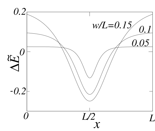
FIG. 2.: The spatial distribution of the electrical field in the F-wire for different values of $w/L$. Here $\Delta\tilde{E}=(E(x)-E_{0})/(2\lambda)^{2}$.

B Large Exchange Energy

Now we consider the case with a large exchange energy or a slow variation of the direction of the magnetization within the DW ($w\gg\sqrt{D/J}$). In this case, the problem becomes more complicated because we cannot neglect the commutator on the left hand side in Eqs. (19,20) and cannot find a solution of these equations even for the case of small $\lambda$. Therefore we simplify the problem assuming that the shape of the DW is described by a piece-wise linear function (see Fig. 1)

$$\mbox{$\hat{n}$}=\left\{\begin{array}[]{cr}\hat{\sigma}_{3}&{\rm in\;region\;I}\\ \hat{\sigma}_{3}\exp[-i(\pi/w)(x-(L-w)/2)\hat{\sigma}_{1}]&{\rm within\;the\;DW}\\ -\hat{\sigma}_{3}&{\rm in\;region\;III.}\end{array}\right.$$ (46)

Obviously the results for other shapes of the DW like that given by Eq. (44) will differ from ours only by a numerical factor. We again expand the solution in the small parameter $\lambda$, i.e. $\mbox{$\hat{a}$}=\mbox{$\hat{a}$}_{0}+\mbox{$\hat{a}$}_{1}+\mbox{$\hat{a}$}_{2}+...$. The zeroth order terms can be obtained easily as before and they are given by Eqs.(32,33). The first correction $\mbox{$\hat{a}$}_{1}$ is given again by Eq. (35) and the first correction for the symmetric part $\mbox{$\hat{s}$}_{1}$ obeys the equation

$$D\partial_{xx}^{2}\mbox{$\hat{s}$}_{1}-iJ[\mbox{$\hat{n}$}(x),s_{1}]=2\lambda\hat{I}_{0}\partial_{x}\mbox{$\hat{n}$}\;.$$ (47)

This equation can be solved for the case of $\mbox{$\hat{n}$}(x)$ given by Eq.(46) with the help of an unitary transformation (a rotation in the spin space). We do not need to find the second order corrections $\mbox{$\hat{a}$}_{2}$ and $\mbox{$\hat{s}$}_{2}$, since the sought correction to the conductance can be expressed in terms of $\mbox{$\hat{s}$}_{1}.$ Indeed, let us write the equation for $\mbox{${\rm Tr}$}\mbox{$\hat{s}$}_{2}$ which follows from Eq.(20)

$$\mbox{${\rm Tr}$}\{D\partial_{x}\mbox{$\hat{s}$}_{2}+(v_{F}/3)[\lambda^{2}\mbox{$\hat{a}$}_{0}+2\lambda\mbox{$\hat{n}$}\mbox{$\hat{a}$}_{1}]-\mbox{$\hat{I}$}_{2}\}=0\;,$$ (48)

where $\mbox{$\hat{I}$}_{2}$ is the integration constant which is related to $\mbox{$\hat{a}$}_{2}:$ $\mbox{${\rm Tr}$}\hat{\sigma}_{0}\mbox{$\hat{a}$}_{2}=-l\mbox{$\hat{I}$}_{2}/D$. We integrate this equation from $0$ to $L$ taking into account the boundary conditions at $x=0$ and $x=L$: $\mbox{$\hat{s}$}_{2}=0.$ After simple transformations we obtain

$$\mbox{${\rm Tr}$}\{\mbox{$\hat{I}$}_{2}-3\lambda^{2}\mbox{$\hat{I}$}_{0}\}/D=2\lambda\mbox{${\rm Tr}$}\hat{\sigma}_{0}\{\int_{0}^{L}dx\mbox{$\hat{s}$}_{1}(x)\mbox{$\hat{n}$}(x)\};.$$ (49)

As before, the correction to the conductance is determined by $\mbox{$\hat{I}$}_{2}.$ We see that in order to find this correction, one has to solve Eq. (47) for $\mbox{$\hat{s}$}_{1}.$ This equation can be solved with the help of the unitary transformation

$$\mbox{$\hat{s}$}_{1}=\hat{U}\cdot\mbox{$\hat{S}$}\cdot\hat{U}^{+},\;\;\hat{U}=\hat{\sigma}_{0}\cos\alpha/2+i\hat{\sigma}_{1}\sin\alpha/2\text{\ \ \ }$$ (50)

This rotation transforms the vector $\hat{n}$ into $\mbox{$\hat{N}$}=\hat{\sigma}_{3}.$ Performing the $U$-transformation, we obtain instead of Eq.(49)

$$\mbox{${\rm Tr}$}\hat{\sigma}_{0}\{\mbox{$\hat{I}$}_{2}-3\lambda^{2}\mbox{$\hat{I}$}_{0}\}/D=2\lambda\partial_{x}\alpha\mbox{${\rm Tr}$}_{\hat{\sigma}}\hat{\sigma}_{2}<\mbox{$\hat{S}$}(x)>\;.$$ (51)

After the $U$-transformation Eq.(47) acquires the form (in the region of the DW)

$$\partial_{xx}^{2}\mbox{$\hat{S}$}-(Q^{2}/2)(\mbox{$\hat{S}$}-\hat{\sigma}_{1}\mbox{$\hat{S}$}\hat{\sigma}_{1})+iQ(\hat{\sigma}_{1}\partial_{x}\mbox{$\hat{S}$}-\partial_{x}\mbox{$\hat{S}$}\hat{\sigma}_{1})-iJ[\mbox{$\hat{N}$},\mbox{$\hat{S}$}]=2\lambda\hat{\sigma}_{2}\mbox{$\hat{I}$}_{0}Q/D\;,$$ (52)

where $Q=\partial_{x}\alpha$ and $\mbox{$\hat{N}$}=\hat{\sigma}_{3}$. This equation is valid in the region of the DW, whereas in the regions I and III we have to set $Q=0$ and to take into account that in the region III $\mbox{$\hat{N}$}=-\hat{\sigma}_{3}.$ The matrix $\hat{S}$ should be represented as a sum: $\mbox{$\hat{S}$}=S_{1}\hat{\sigma}_{1}+S_{2}\hat{\sigma}_{2}+S_{3}\hat{\sigma}_{3}.$ The components $S_{k}$ are given by a linear combination of the eigen-functions of Eq. (52). They obey zero boundary conditions at $x=0$ and $x=L$ and should be matched at $x=L_{1}=(L-w)/2$ and $x=L_{2}=(L+w)/2$. The eigen-values of Eq.(52) ($S_{k}\sim\exp(\kappa x))$ are determined by the equation

$$\kappa^{2}(\kappa^{2}+Q^{2})^{2}=(\kappa^{2}-Q^{2})/\xi_{J}^{2}\;,$$ (53)

where $\xi_{J}^{-2}=2J/D.$ In a general case a solution of Eq. (52) has a cumbersome form. We represent here the form of a solution for $\mbox{${\rm Tr}$}\hat{\sigma}_{2}\mbox{$\hat{S}$}(x)$ in the region of the DW which we are interested in:

$$\mbox{${\rm Tr}$}\hat{\sigma}_{2}\mbox{$\hat{S}$}(x)\cong-2\lambda\mbox{${\rm Tr}$}_{\hat{\sigma}}\mbox{$\hat{I}$}_{0}(\xi_{J}^{2}Q/D)\mathop{\rm Im}[\exp(-(1+i)(x-L_{1})/\xi_{J}\text{\ }\sqrt{2})\text{\ }+\exp((1+i)(x-L_{2})/\xi_{J}\text{\ }\sqrt{2})]\;.$$ (54)

We dropped terms of the higher order in the parameter $Q\xi_{J}$ $\sim\xi_{J}/w.$ Using this expression and Eq. (51), we readily get the expression for the current and for the conductance $G$

$$G=G_{1d}\left(1-\frac{\pi^{2}\xi_{J}^{3}}{Lw^{2}}\lambda^{2}\right)\;,$$ (55)

where $G_{1d}$ is the conductance for a homogenous magnetized wire (see Eq. (27)). Again terms of order higher than $\lambda^{2}$ should be neglected. Note that $G_{1d}$ is always larger than the conductance in the case of a two domain wire $G_{2d}$ (see Eq. (30)). Eq. (55) shows that the DW decreases the conductance compared to the conductance $G_{1d}$ of a single domain F wire. Our result is sketched in Fig. 3. We see that within our approach a DW with a finite width is always a source of resistance.

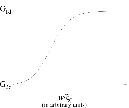
FIG. 3.: Schematical representation of the conductance as a function of the width $w$ of the DW. In the intermediate region (dashed line) the curve is extrapolated from our results.

IV Conclusion

Using a simple microscopic model (equal density-of-states but different impurity scattering times $\tau_{\uparrow,\downarrow}$ for electrons with spin up and down), we have derived the kinetic equation for the matrix distribution function. The derivation has been performed by a standard method on the basis of microscopic equations for the quasiclassical Green functions in the Keldysh technique. This equation can be applied to the studies of transport in, for example, ferromagnets with a non-homogeneous magnetization.

We have employed this equation to calculate the conductance $G$ in a mesoscopic F’/F/F’ structure. We have assumed that the parameter $\lambda=(\tau_{\downarrow}-\tau_{\uparrow})/$ $2(\tau_{\downarrow}+\tau_{\uparrow})$ is small and the length of the F wire $L$ is shorter than the spin energy relaxation length. Two different limits appear which are determined by the product of the exchange energy $J$ and the diffusion time $\tau_{w}=w^{2}/D$ of electrons through the DW. In the limit $\tau_{w}J\ll 1$ and a very thin DW the conductance of the structure (per the unit cross-section area) is equal to $G_{2d}=4\sigma_{\uparrow}\sigma_{\downarrow}(\sigma_{\uparrow}+\sigma_{\downarrow})/L$. The account for a finite width of the DW leads to an increase in the conductance by a normalized amount of the order ($\lambda w/L)^{2}.$ We have also calculated in this limit the spatial distribution of the electric field in the F wire. The electric field has a minimum in the center of the DW which corresponds to an enhanced local conductivity. In the other limit $\tau_{w}J>>1$ (adiabatic variation of the magnetization in the DW) the conductance coincides in the main approximation with that of a single domain structure $G_{1d}=(\sigma_{\uparrow}+\sigma_{\downarrow})/L$. The account for rotation of the magnetization in the DW leads to a negative correction to the conductance of the order -$\lambda^{2}(\tau_{w}J)^{-3/2}(w/L).$ Our results differ from those published earlier [12, 13, 17] because in the latter works the collision term was written phenomenologically. In particular the matrix character of the impurity vertex was not taken into account.

We would like to thank SFB 491 for financial support.

REFERENCES

- [1] J. F. Gregg, W. Allen, K. Ounadjela, M. Viret, M. Hehn, S. M. Thompson, and J. M. D. Coey, Phys. Rev. Lett. 77, 1580 (1996).
- [2] U. Ebels, A. Radulescu, Y. Henry, L. Piraux, and K. Ounadjela, Phys. Rev. Lett. 84, 983 (2000).
- [3] U. Rudiger, J. Yu, L. Thomas, S. S. P. Parkin, and A. D. Kent, Phys. Rev. B 59, 11914 (1999).
- [4] R. Danneau, P. Warin, J. P. Attane, I. Petej, C. Beigne, C. Fermon, O. Klein, A. Marty, F. Ott, Y. Samson, and M. Viret, Phys. Rev. Lett. 88, 157201 (2002).
- [5] T. Taniyama, I. Nakatani, T. Namikawa, and Y. Yamazaki, Phys. Rev. Lett. 82, 2780 (1999).
- [6] U. Rudiger, J. Yu, S. Zhang, and A. D. Kent, Phys. Rev. Lett. 80, 5639 (1998).
- [7] J. Smit, Physica 16, 612 (1951).
- [8] L. Berger, Physica 30, 1141 (1964).
- [9] R. I. Potter, Phys. Rev. B 10, 4626 (1974).
- [10] G. Tatara and H. Fukuyama, Phys. Rev. Lett. 78, 3773 (1997).
- [11] Yuli Lyanda-Geller, I. L. Aleiner, and Paul M. Goldbart, Phys. Rev. Lett. 81, 3215 (1998).
- [12] P. M. Levy and S. Zhang, Phys. Rev. Lett. 79, 5110 (1997).
- [13] E. Simanek, Phys. Rev. B 63, 224412 (2001).
- [14] R. P. van Gorkom, A. Brataas, and G. E. W. Bauer, Phys. Rev. Lett. 83, 4401 (1999).
- [15] L. R. Tagirov, B. P. Vodopyanov, and K. B. Efetov, Phys. Rev. B 63, 104428 (2001).
- [16] P. Bruno, Phys. Rev. Lett. 83, 2425 (1999).
- [17] V. K. Dugaev, J. Barnas, A. Lusakowski, and L. A. Turski, cond-mat/0201338 .
- [18] F. S. Bergeret, A. F. Volkov, and K. B. Efetov, Phys. Rev. B 64, 134506 (2001).
- [19] A. I. Larkin and Y. N. Ovchinnikov, in Nonequilibrium Superconductivity, edited by D. N. Langenberg and A. I. Larkin (Elservier, Amsterdam, 1984).
- [20] A. Abrikosov, Fundamentals of the theory of Metals (North-Holland, Holland, 1988).
- [21] A. Abrikosov, L. Gorkov, and I. Dzyaloshinski, Methods of Quatum Field Theory in Statistical Physics (Dover Publications, New York, 1963).
- [22] L. D. Landau and E. M. Lifshitz, Phys. Z. Sowjetunion 8, 153 (1935).