Effect of initial correlations on short–time decoherence

Abstract

We study the effect of initial correlations on the short–time decoherence of a particle linearly coupled to a bath of harmonic oscillators. We analytically evaluate the attenuation coefficient of a Schrödinger cat state both for a free and a harmonically bound particle, with and without initial thermal correlations between the particle and the bath. While short–time decoherence appears to be independent of the system in the absence of initial correlations, we find on the contrary that, for initial thermal correlations, decoherence becomes system dependent even for times much shorter than the characteristic time of the system. The temperature behavior of this system dependence is discussed.

Environment induced decoherence plays a fundamental role in many areas, ranging from quantum cosmology [1] and the theory of quantum measurement [2] to quantum information and quantum computing [3]. Experimental investigations of the decoherence process have recently been reported in Refs. [4, 5, 6]. Environmental decoherence can be defined as ”… the (irreversible) loss of quantum coherence of a quantum system due to its coupling to an environment” [7]; it manifests itself in the dynamical suppression of interference phenomena [8, 9]. A simple way to quantify the destruction of coherence is thus to consider the superposition of two localized wave packets (Schrödinger cat state) and to look at the decay of the interference term, as measured for instance by the attenuation coefficient [see Eq. (20) below]. An important characteristic of decoherence is that it occurs on a very fast time scale, usually much shorter than the energy dissipation scale. We note that the short–time limit of decoherence has recently attracted a renewed interest in the literature [10, 11, 12, 13, 14]. Interestingly, Braun, Haake and Strunz [12, 13] have identified a new regime of fast decoherence beyond the usual Golden Rule regime. In this limit of large separations between the wave packets (interaction-dominated decoherence), quantum decoherence appears independent of both the system and the heat bath.

Most studies of environment induced decoherence make use of the simplified assumption that the system and the bath are initially uncorrelated [15]. Then, the initial composite density operator for system plus bath can be factorized into a product of a system operator and a bath operator. However, in the general, and more realistic case, initial correlations can be present and the latter might affect the decoherence process, especially at very short times as first pointed out by Romero and Paz [16]. In fact, as recently shown by Ford, Lewis and O’Connell [10, 11], initial thermal conditions can dramatically modify the decoherence rate. They find that the decoherence time for an unbound particle becomes independent of the strength of the dissipation when it is initially at the same temperature as the bath. Our aim in this paper is to complement the discussion of the effect of initial thermal correlations on short–time decoherence by analytically comparing the attenuation factor of a free particle with that of a harmonic oscillator, with and without thermal initial correlations. As our main tool, we shall employ the by now standard model of a system linearly coupled to a bath of harmonic oscillators. This model is exactly solvable and the exact reduced density operator of the quantum system is conveniently obtained within a path integral approach [17]. This model has been extensively used in decoherence studies for the case of factorizable initial conditions, building up on the work of Caldeira and Leggett [18]. It has been extended later on to correlated thermal initial conditions by Hakim and Ambegaokar for a free particle [19] and by Morais Smith and Caldeira for a harmonically bound particle [20, 21] (see also the work of Grabert and collaborators [22]). In the following we shall use the exact results derived by Morais Smith and Caldeira [21] to compute the time evolution of the superposition of two Gaussian wave packets separated by a distance $2a$ and of width $b$, $\psi(x)=c_{1}\exp[-(x-a)^{2}/4b^{2}]+c_{2}\exp[-(x+a)^{2}/4b^{2}]$. The corresponding initial density operator, $\rho_{S}(x,y,0)=\psi(x)\psi^{*}(y)$, is given by

$$\rho_{s}(x,y,0) = |c_{1}|^{2}\exp\Big{[}-\frac{(x-a)^{2}+(y-a)^{2}}{4b^{2}}\Big{]}$$ (1)

$$+ |c_{2}|^{2}\exp\Big{[}-\frac{(x+a)^{2}+(y+a)^{2}}{4b^{2}}\Big{]}$$ (2)

$$+ c_{1}c_{2}^{*}\exp\Big{[}-\frac{(x-a)^{2}+(y+a)^{2}}{4b^{2}}\Big{]}$$ (3)

$$+ c_{1}^{*}c_{2}\exp\Big{[}-\frac{(x+a)^{2}+(y-a)^{2}}{4b^{2}}\Big{]}\ .$$ (4)

We calculate the short–time limit of the attenuation coefficient for a harmonically bound particle with and without initial thermal correlations and compare the obtained results with those of a free particle. We find that for initial decorrelation, the attenuation coefficient is identical for both the free particle and the linear oscillator, that is to say, decoherence is independent of the nature of the system. On the other hand, for initial thermal correlations, we find that the attenuation coefficient acquires a system dependent part, even for times much smaller than the characteristic time of the system. This shows that in the presence of initial thermal correlations decoherence is system dependent. At very high temperature, this system dependence turns out to be negligibly small. However, in the opposite limit of low temperature, it becomes increasingly important.

The model. We consider a particle of unit mass, moving in an external potential $V(x)$ and linearly coupled through its position to a set of independent harmonic oscillators with mass $m_{i}$ and frequency $\omega_{i}$. The composite Hamiltonian is written in the form

$$H = \frac{p^{2}}{2}+V(x)+\sum_{i}x\,C_{i}x_{i}+\sum_{i}\left(\frac{p^{2}_{i}}{2m_{i}}+\frac{1}{2}m_{i}\omega_{i}^{2}x_{i}^{2}\right)$$ (6)

$$+\sum_{i}x^{2}\frac{C_{i}^{2}}{2m_{i}\omega_{i}^{2}}\ ,$$

where the $C_{i}$’s are coupling constants. In the limit of infinitely many oscillators, the bath is entirely characterized by the spectral density function,

$$I(\omega)=\frac{\pi}{2}\sum_{i}\frac{C_{i}^{2}}{m_{i}\omega_{i}}\,\delta(\omega-\omega_{i})=2\gamma\omega\,\theta(w-\omega_{c})\ ,$$ (7)

where the last equality defines Ohmic damping with damping coefficient $\gamma$. Here $\omega_{c}$ is a cutoff frequency that will be replaced by infinity in all convergent integrals. The reduced density operator $\rho_{S}(t)$ of the system at time $t$ is obtained after tracing out the bath degrees of freedom. In coordinate representation it reads

$$\rho_{S}(x,y,t)= \int dx^{\prime}dy^{\prime}d{\bf R}d{\bf R^{\prime}}d{\bf Q^{\prime}}\,K(x,{\bf R},t;x^{\prime},{\bf R^{\prime}},0)$$ (9)

$$\times K^{*}(y,{\bf R},t;y^{\prime},{\bf Q^{\prime}},0)\langle x,{\bf R^{\prime}}|\rho(0)|y^{\prime},{\bf Q^{\prime}}\rangle\ .$$

Here ${\bf R}$, ${\bf R^{\prime}}$ and ${\bf Q^{\prime}}$ collectively denote the coordinates of the bath, $K$ is the propagator and $\rho(0)$ the initial density operator of the composite system. If we assume that at $t=0$ the system and the bath are uncoupled and that the latter is in thermal equilibrium, then the initial density operator can be written as $\rho_{0}(x^{\prime},{\bf R^{\prime}};y^{\prime},{\bf Q^{\prime}})=\rho_{S}(x^{\prime},y^{\prime},0)\rho_{eq}({\bf R^{\prime}},{\bf Q^{\prime}})$, where $\rho_{S}(x^{\prime},y^{\prime},0)$ describes the initial state of the system and $\rho_{eq}({\bf R^{\prime}},{\bf Q^{\prime}})$ is the equilibrium density operator of the bath. On the other hand, if the system and the bath are initially coupled and in thermal equilibrium with each other, $\rho(0)$ cannot be factorized into a product of a system and a bath operator anymore. Instead, we have $\rho_{0}(x^{\prime},{\bf R^{\prime}};y^{\prime},{\bf Q^{\prime}})=\rho_{S}(x^{\prime},y^{\prime},0)\rho_{eq}(x^{\prime},y^{\prime},{\bf R^{\prime}},{\bf Q^{\prime}})$, where $\rho_{eq}(x^{\prime},y^{\prime},{\bf R^{\prime}},{\bf Q^{\prime}})$ is now the equilibrium density operator of the composite system. We shall refer to these two cases as (i) uncorrelated initial conditions and (ii) thermal initial conditions, respectively. We mention that other correlated initial conditions have also been considered (see Refs. [20, 21, 22]). The integrals over ${\bf R}$, ${\bf R^{\prime}}$ and ${\bf Q^{\prime}}$ in Eq. (9) can now be performed exactly, yielding

$$\rho_{S}(q,\xi,t)=\int dq^{\prime}d\xi^{\prime}\,J(q,\xi,t;q^{\prime},\xi^{\prime},0)\,\rho_{S}(q^{\prime},\xi^{\prime},0)\ ,$$ (10)

where we have introduced the center of mass and relative coordinates $q=(x+y)/2$ and $\xi=x-y$. The dynamics of the particle is completely determined by the propagating function $J(q,\xi,t;q^{\prime},\xi^{\prime},0)$. Equation (10) can be considered as the full solution of the master equation describing the time evolution of the dissipative particle with (and without) thermal initial conditions. In the diagonal case $\xi=0$, the propagator $J$ is given by (we put $\hbar\!=\!k_{B}\!=\!1$ throughout the paper),

$$J(q,0,t;q^{\prime},\xi^{\prime},0)= \frac{N(t)}{2\pi}\,\exp\Big{[}i\Big{(}\alpha(t)\,q^{\prime}\xi^{\prime}-N(t)\,q\xi^{\prime}\Big{)}\Big{]}$$ (12)

$$\times\exp\Big{[}-\Big{(}\varepsilon\,q^{\prime 2}+\Delta(t)\,\xi^{\prime 2}\Big{)}\Big{]}\ ,$$

with

$$\alpha(t) = K(t)+\gamma-2\varepsilon E(t)\ ,$$ (13)

$$\Delta(t) = C(t)-\varepsilon E(t)^{2}\ ,$$ (14)

$$\mbox{and }\hskip 28.45274pt\varepsilon = \frac{\beta}{2\kappa}\ .$$ (15)

The exact expressions for the coefficients $K(t)$, $N(t)$, $C(t)$ and $E(t)$ have been derived in Ref. [21] for a linear oscillator with frequency $\omega_{0}$ initially in thermal equilibrium with a heat bath at inverse temperature $\beta=1/T$. They are reproduced in the appendix for completeness. Remarkably, the form of the propagating function (12) remains the same for uncorrelated initial conditions, as well as for a free particle. The case of uncorrelated initial conditions is recovered by setting $\varepsilon$ to zero and keeping only the first double integral in $C_{\omega}(t)$, Eq. (25), [$K(t)$ and $N(t)$ being unchanged], while the unbound particle is obtained by letting the frequency $\omega_{0}$ go to zero [21]. The quantity $\kappa$ that appears in Eq. (9) is equal to the variance of the position $\langle x^{2}\rangle_{eq}$ in equilibrium [see Eq. (36) in appendix A]. The factor $\varepsilon$ ($=1/2\lambda$ in the notation of [21]), which stems from the initial thermal correlations, will turn out to be important in the following discussion. Its asymptotic behavior at high ($T\!\gg\!\omega_{0}$) and low temperature ($T\!\ll\!\omega_{0}$) is respectively given by $\varepsilon\sim(\beta\omega_{0})^{2}/2\ll 1$ and $\varepsilon\sim\beta\omega_{0}\gg 1$. The diagonal density operator of the system at time $t$ can then be easily obtained by combining Eqs. (1), (10) and (12). We find

$$\rho_{S}(q,0,t) \sim \exp\Big{[}-\frac{2b^{2}(Nq-a\alpha)^{2}+a^{2}(1+8b^{2}\Delta)\varepsilon}{\sigma^{2}}\Big{]}$$ (16)

$$+ \exp\Big{[}-\frac{2b^{2}(Nq+a\alpha)^{2}+a^{2}(1+8b^{2}\Delta)\varepsilon}{\sigma^{2}}\Big{]}$$ (17)

$$+ 2\exp\Big{[}-\frac{a^{2}(4\Delta+2b^{2}\alpha^{2})+2b^{2}N^{2}q^{2}}{\sigma^{2}}\Big{]}$$ (19)

$$\times\cos\frac{2aNq(1+2b^{2}\varepsilon)}{\sigma^{2}}\ ,$$

where we have defined $\sigma^{2}=(1+8b^{2}\Delta)(1+2b^{2}\varepsilon)+4b^{4}\alpha^{2}$ (for simplicity, we have put $c_{1}$ equal to $c_{2}$). Equation(16) is written as a sum of three terms. The first two terms correspond to two separately propagating wave packets, while the third one, containing the cosine, is an interference term. The attenuation coefficient $a(t)$ is defined as the ratio of the factor multiplying the cosine to twice the geometric mean of the first two terms. It follows from Eq. (16) that

$$a(t)=\exp\Big{[}\frac{-4a^{2}\Delta+a^{2}(1+8b^{2}\Delta)\varepsilon}{\sigma^{2}}\Big{]}\ .$$ (20)

This expression is still exact. The attenuation factor(20) is the measure of decoherence we shall use in what follows to investigate the short–time limit of decoherence. To be more specific, we shall place ourselves in the limit of weak coupling between the system and the bath, $\gamma\ll\omega_{0}$, and assume that the time is small compared to the relaxation time, $\gamma t\ll 1$ and also small compared to the evolution time of the harmonic oscillator, $\omega_{0}t\ll 1$.

Uncorrelated initial conditions. We begin by considering initial decorrelation between the system and the heat bath. Physically, this corresponds to the situation where the system and the bath are isolated prior to their coupling at $t=0$, the system being effectively at zero temperature. In this case $\varepsilon=0$, $\alpha(t)=N(t)$ and $\Delta(t)=C(t)$ (with only the first double integral). In the high–temperature limit, $T\!\gg\!\gamma,\omega_{0}$, we approximate the hyperbolic cotangent in Eq. (37) by $\mbox{\ coth }x\simeq 1/x$. Expanding $\alpha(t)$ and $\Delta(t)$, Eqs. (7) and (8), in lowest order in time, we find that the attenuation coefficient (20) is given by

$$a_{0}^{\scriptscriptstyle{FP}}(t)=\exp\Big{[}-\frac{4a^{2}T\gamma t^{3}}{12b^{4}+8b^{2}T\gamma t^{3}+3t^{2}}\Big{]}\ ,$$ (21)

for the free particle ($t\!\ll\!\gamma^{-1}$), and by

$$a_{0}^{\scriptscriptstyle{OH}}(t)=\exp\Big{[}-\frac{4a^{2}T\gamma t^{3}}{12b^{4}+8b^{2}T\omega_{0}^{2}\gamma t^{3}+3t^{2}}\Big{]}\ ,$$ (22)

for the harmonic oscillator ($t\!\ll\!\omega_{0}^{-1}$). For very short times, we thus obtain the same attenuation coefficient for both the free particle and the linear oscillator,

$$a_{0}(t)\simeq\exp\Big{[}-\frac{a^{2}T\gamma t^{3}}{3b^{4}}\Big{]}\ .$$ (23)

Interference patterns between the two superposed wave packets are hence destroyed according to a stretched exponential on a time scale, $\tau_{D}\!=\!(3b^{4}/\gamma Ta^{2})^{1/3}$. The decoherence time $\tau_{D}$ depends solely on the friction strength $\gamma$, the temperature $T$ and the parameters of the initial wave packets (separation $a$ and width $b$), and not on any system specific quantity, like the frequency of the oscillator for example. Since we look at times much shorter than the characteristic time of the system, $\tau_{S}\sim\omega_{0}^{-1}$, such a system independence of the decoherence time is to be expected. However, as we shall see, this is only true for uncorrelated initial conditions. This result is reminiscent of the universal regime discussed by Haake and coworkers, where the decoherence rate was also found to be independent of the nature of the system [12, 13]. However, the short–time attenuation factor (23) does not quite belong to this regime of very fast decoherence characterized by a Gaussian decay law, $\exp[-(t/\tau_{D})^{2}]$. On the other hand, the cubic time dependence clearly indicates that expression (23) goes beyond the (long-time) Golden Rule regime, $t\!\gg\!\omega_{0}^{-1}$, and its typical exponential decay, $\exp[-t/\tau_{D}]$. Here we have a much slower initial decoherence compared to the Golden Rule expression. A similar short–time cubic dependence of the decoherence factor already appears in Refs. [18] and [23]. We also mention that the short-time approximation used in the derivation of Eq. (23) amounts to neglecting the spreading of the wave packet that appears in the denominator of the attenuation coefficient. For instance, the short-time spreading of the free wave packet in Eq. (21) is given by $\langle\Delta x^{2}(t)\rangle=b^{2}+t^{2}/4b^{2}+2T\gamma t^{3}/3$, which reduces to the initial width $b^{2}$ for very short times.

Thermal initial conditions. We now turn to the case where the system and the bath are initially correlated and in thermal equilibrium. First, it should be realized that thermal initial conditions not only modify the coherence time of the system, they also directly affect the overall coherence length [13]. As a matter of fact, we easily see from the coordinate representation of the free particle equilibrium density matrix, $\langle x|\exp[-\beta p^{2}/2]|y\rangle\simeq\exp[-(x-y)^{2}/2\beta]$, that there is an exponential cutoff in $x-y$ over distances of the order of the thermal de Broglie wavelength, $\lambda\sim 1/\sqrt{T}$. The two wave packets can therefore only coherently interfere if they are separated by a distance smaller than $\lambda$. This distance is extremely small at high temperature, but becomes appreciable when the temperature is very low.

In the limit of high temperature, we can compute the attenuation factor (20) for the free particle, for times smaller than the relaxation time, $t\ll\gamma^{-1}$, by expanding the functions $\alpha(t)$ and $\Delta(t)$ up to lowest order in $t$, in analogy with the previous section (now keeping all the terms). For very short times, this leads to

$$a_{hT}^{\scriptscriptstyle{FP}}(t) = \exp\Big{[}-\frac{2a^{2}Tt^{2}}{4b^{4}+4Tb^{2}t^{2}+t^{2}}\Big{]}$$ (24)

$$\simeq \exp\Big{[}-\frac{a^{2}Tt^{2}}{2b^{4}}\Big{]}\ .$$ (25)

The short–time expression (24) is equivalent to the result recently obtained by Ford, Lewis and O’Connell using an exact method based on quantum distribution functions [11]. It is worth noticing that Ford and O’Connell have also derived Eq. (24) with a more elementary method making only use of basic quantum mechanics and equilibrium statistical mechanics [10]. This approximate method is valid in the limit of vanishingly small friction. Equation (24) shows that, in the presence of initial thermal correlations between the system and the bath, the short–time dependence of the exponent of the decoherence coefficient is now quadratic. This has to be contrasted with the cubic dependence obtained for initial decorrelation in Eq. (23). Moreover, the decoherence time, $\tau_{D}=(2b^{4}/Ta^{2})^{1/2}$, appears to be independent of the friction coefficient $\gamma$. This remarkable result indicates that at high temperature, decoherence can occur without dissipation [10, 11].

Similarly, the attenuation coefficient for the harmonic oscillator can be calculated in the limit $t\ll\omega_{0}^{-1}$. Still in the high–temperature limit, we find that for very short times it is given by

$$a_{hT}^{\scriptscriptstyle{OH}}(t) = \exp\Big{[}-\frac{2a^{2}T\omega_{0}^{2}t^{2}+a^{2}\varepsilon(4b^{2}T\omega_{0}^{2}t^{2})}{4\omega_{0}^{2}b^{4}+4b^{2}T\omega_{0}^{2}t^{2}+\omega_{0}^{2}t^{2}}\Big{]}$$ (26)

$$\simeq \exp\Big{[}-\frac{a^{2}Tt^{2}}{2b^{4}}(1+2b^{2}\varepsilon)\Big{]}\ ,$$ (27)

with $\varepsilon\simeq(\beta\omega_{0})^{2}/2$. Contrary to Eq. (23), we observe that for initial thermal conditions, the short–time attenuation coefficients for the free particle (24) and the harmonically bound particle (26) are not identical, even for times much smaller than the characteristic system time $\tau_{S}$. Equation (26) indeed contains an additional, system specific correction, that depends on the frequency of the linear oscillator $\omega_{0}$, and on the temperature $T$. This term finds its origin in the initial thermal correlations existing between the system and the heat bath at $t=0$ (see the discussion below). In the limit of high temperature, $T\!\gg\!\omega_{0}$, this correction, which is proportional to $\varepsilon$, is negligibly small. However, as we shall see next, it becomes increasingly important as the temperature is lowered.

In the low–temperature limit, we replace the hyperbolic cotangent in Eq. (37) by unity, $\mbox{\ coth }x\simeq 1$. For very short times, we find that the attenuation coefficient for the free particle reads ($t\!\ll\!\gamma^{-1}$),

$$a_{lT}^{\scriptscriptstyle{FP}}(t) = \exp\Big{[}\frac{a^{2}\gamma}{\pi b^{4}}(\ln\gamma t+\gamma_{e}-3+\ln 2)t^{2}\Big{]}$$ (28)

$$\simeq \exp\Big{[}\frac{a^{2}}{\pi b^{4}}\gamma t^{2}\ln\gamma t\Big{]}\ ,$$ (29)

where $\gamma_{e}$ is Euler’s constant. We note that in contrast to the high–temperature expression (24), Eq. (28) now explicitly contains the damping coefficient $\gamma$ (see the recent discussion in Ref. [24] on this point). We also note that the exponent in Eq. (28) is actually negative since $\gamma t<1$. The ”$t^{2}\ln t$” behavior of the decoherence factor in Eq. (28) is consistent with the result found by Romero and Paz for the superposition of two translations [16]. In an analogous way, we find that the short–time expression of the attenuation coefficient for the linear oscillator is given by ($t\!\ll\!\omega_{0}^{-1}$),

$$a_{lT}^{\scriptscriptstyle{OH}}(t) = \exp\Big{[}\frac{2a^{2}\gamma}{\pi b^{4}}(\ln\omega_{0}t+\gamma_{e})t^{2}(1+2b^{2}\varepsilon)\Big{]}$$ (30)

$$\simeq \exp\Big{[}\frac{2a^{2}}{\pi b^{4}}\gamma t^{2}\ln\omega_{0}t(1+2b^{2}\varepsilon)\Big{]}\ ,$$ (31)

where now $\varepsilon\simeq\beta\omega_{0}$. In the limit of low temperature, $T\ll\omega_{0}$, $\varepsilon$ becomes very large. It should be noticed that the factor $\ln\gamma t$ in Eq. (28) comes from the first double integral in $C_{\omega}(t)$, Eq. (25), whereas the factor $\ln\omega_{0}t$ in Eq. (30) comes from the next two single integrals of (25).

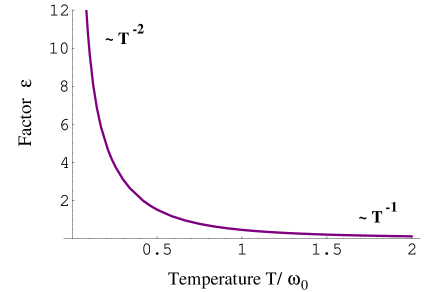
FIG. 1.: Temperature dependence of the factor $\varepsilon$, given by Eq. (32), in the limit of small friction, $\gamma\ll\omega_{0}$.

Discussion. From a technical point of view, the inclusion of initial correlations between the system and the bath results in a modification of the integration contour in the complex–time plane (Keldish contour) that appears in the path integral evaluation of the influence functional [20, 21, 22]. More precisely, the effect of the initial correlations is to couple the forward and backward integration paths along the real time axis through an imaginary path along the Euclidean time axis, $\tau=it$. This leads to additional terms in the influence functional that are given by Euclidean integrals of the form$\int_{0}^{\beta}d\tau f(\tau)$. The presence of the factor $\varepsilon$ in the propagating function (12) can be directly traced back to these terms. Clearly, even for very short times, when the dynamics of the system can be completely neglected, some of these terms, that depend only on temperature and not on time, will still be present. For initial thermal correlations, these terms explicitly depend on the nature of the system through the common initial equilibrium state of the system with the bath. As a consequence, even for arbitrarily small times, the attenuation coefficient will be system dependent. Only in the special case of uncorrelated initial conditions is the attenuation factor system independent at short times. It turns out, furthermore, that the contribution of these system–specific terms to the decoherence time will be negligibly small in the limit of high temperature, $\beta\rightarrow 0$, (as easily seen from the Euclidean integral above) and will become very important in the opposite limit of low temperature, $\beta\rightarrow\infty$. This general discussion confirms the results obtained for the special examples of a free particle and a linear oscillator.

Finally, it is also interesting to look at the temperature dependence of the factor $\varepsilon$ which can be written in the form

$$\varepsilon=\left[\frac{4\gamma}{\pi\beta}\int_{0}^{\infty}d\omega\frac{\omega\coth(\beta\omega/2)}{(\omega^{2}-\omega_{0}^{2})^{2}+4\gamma^{2}\omega^{2}}\right]^{-1}\ .$$ (32)

At high temperature, $\varepsilon$ asymptotically decays to zero as $T^{-1}$, whereas at low temperature it diverges as $T^{-2}$ [see Figure (1)]. In the absence of damping, Eq. (32) reduces to the simple expression

$$\varepsilon=\frac{\beta\omega_{0}}{\coth(\beta\omega_{0}/2)},\hskip 28.45274pt\gamma=0\ .$$ (33)

We see from Eq. (33) that the high–temperature limit $\beta\rightarrow 0$ is formally equivalent to the free particle limit $\omega_{0}\rightarrow 0$. This offers another explanation why the system dependent correction to the attenuation coefficient becomes vanishingly small at high temperature. Moreover, the presence of the hyperbolic cotangent in the denominator of Eq. (33) hints at a possible connection between the divergence of $\varepsilon$ close to zero temperature and zero–point oscillations of the bath.

In conclusion, we have examined the effect of initial correlations on the short–time decoherence of a superposition of two Gaussian wave packets. To this end, we have calculated the attenuation coefficient for both a free particle and a linear oscillator, with and without initial thermal correlations. We have found that for factorizable initial conditions, the attenuation factor, and accordingly the decoherence time, is system independent at very short times. On the other hand, for correlated thermal initial conditions, not only the temporal properties of decoherence are modified —changing from a stretched exponential to a Gaussian decay — but also the coherence length is affected. The latter is of the order of the de Broglie thermal wavelength. Moreover, the attenuation factor now has a system dependent term, containing the frequency of the oscillator and the temperature, and this even at times much smaller than the system characteristic time $\tau_{S}\sim\omega_{0}^{-1}$. The system specific correction to the attenuation coefficient is small in the high temperature limit, where zero–point fluctuations are neglected, but becomes more and more important as the temperature is lowered.

This work was funded in part by the ONR under contract N00014-01-1-0594.

Appendix A

In this appendix we collect for convenience the exact expressions of the quantities appearing in the propagator (12). The derivation of these quantities can be found in Ref. [21]. The functions $K(t)$ and $N(t)$ are given by

$$K(t) = \nu\mbox{ cotan }\nu t\ ,$$ (34)

$$N(t) = \frac{\nu\exp[\gamma t]}{\sin\nu t}\ ,$$ (35)

where $\nu=(\omega_{0}^{2}-\gamma^{2})^{1/2}$. We work in the limit of an underdamped oscillator where the friction coefficient $\gamma$ is smaller than the frequency $\omega_{0}$ of the harmonic oscillator. For a free particle, $\omega_{0}=0$, one has to replace $\nu\rightarrow i\gamma$. The variance of the position in equilibrium, $\kappa=\langle x^{2}\rangle_{eq}$, is given by [22]

$$\kappa=\frac{2\gamma}{\pi}\int_{0}^{\infty}d\omega\frac{\omega\coth(\beta\omega/2)}{(\omega^{2}-\omega_{0}^{2})^{2}+4\gamma^{2}\omega^{2}}\ .$$ (36)

Its asymptotic behavior at high ($T\!\gg\!\omega_{0}$) and low temperature ($T\!\ll\!\omega_{0}$) is respectively given by $\kappa\sim 1/\beta\omega_{0}^{2}$ and $\kappa\sim 1/2\omega_{0}$. The functions $C(t)$ and $E(t)$ are, on the other hand, of the form

$$f(t)=\frac{\gamma}{\pi}\int_{0}^{\omega_{c}}d\omega\,\omega\coth(\beta\omega/2)f_{\omega}(t)\ ,$$ (37)

where $f_{\omega}(t)$ has respectively to be replaced by

$$C_{\omega}(t) = \frac{1}{\sin^{2}\nu t}\int_{0}^{t}dt^{\prime}\int_{0}^{t}dt^{\prime\prime}\sin\nu(t-t^{\prime})\cos\omega(t^{\prime}-t^{\prime\prime})\sin\nu(t-t^{\prime\prime})\exp[\gamma(t^{\prime}+t^{\prime\prime})]$$ (38)

$$+ \frac{4\gamma\omega^{2}}{(\omega_{0}^{2}-\omega^{2})^{2}+4\gamma^{2}\omega^{2}}\frac{1}{\sin\nu t}\int_{0}^{t}dt^{\prime}\cos\omega t^{\prime}\sin\nu(t-t^{\prime})\exp[\gamma t^{\prime}]$$ (39)

$$- \frac{2\omega(\omega^{2}-\omega_{0}^{2})}{(\omega_{0}^{2}-\omega^{2})^{2}+4\gamma^{2}\omega^{2}}\frac{1}{\sin\nu t}\int_{0}^{t}dt^{\prime}\sin\omega t^{\prime}\sin\nu(t-t^{\prime})\exp[\gamma t^{\prime}]+\frac{\omega^{2}}{(\omega_{0}^{2}-\omega^{2})^{2}+4\gamma^{2}\omega^{2}}\ ,$$ (40)

$$E_{\omega}(t) = \frac{2}{\sin\nu t}\frac{1}{(\omega_{0}^{2}-\omega^{2})^{2}+4\gamma^{2}\omega^{2}}\int_{0}^{t}dt^{\prime}\sin\nu(t-t^{\prime})\exp[\gamma t^{\prime}]\Big{(}(\omega_{0}^{2}-\omega^{2})\cos\omega t^{\prime}-2\gamma\omega\sin\omega t^{\prime}\Big{)}\ .$$ (41)

Appendix B

In this appendix we evaluate the function $\widetilde{C}(t)=\sin^{2}\nu t\,C(t)$ [the contributions coming from the function $E(t)$ are of higher order and can therefore be neglected in the limit considered in the paper]. We begin by computing the first double integral in Eq. (25). Introducing the new variables $u=(t^{\prime}+t^{\prime\prime})/2$ and $v=t^{\prime}-t^{\prime\prime}$, we have

$$a_{\omega}(t) = \int_{0}^{t}dt^{\prime}\int_{0}^{t}dt^{\prime\prime}\sin\nu(t-t^{\prime})\sin\nu(t-t^{\prime\prime})\cos\omega(t^{\prime}-t^{\prime\prime})\exp[\gamma(t^{\prime}+t^{\prime\prime})]$$ (42)

$$= \int_{0}^{t}du\int_{0}^{t}dv\sin\nu(t-u-v/2)\sin\nu(t-u+v/2)\exp[2\gamma u]\cos\omega v\ .$$ (43)

The integral over $u$ is readily obtained as,

$$\int_{0}^{t}du\,\sin\nu(t-u-v/2)\sin\nu(t-u+v/2)e^{2\gamma u}=\frac{1}{4}\Big{[}\frac{(e^{2\gamma t}-1)\cos\nu v}{\gamma}+\frac{\gamma\cos 2\nu t-\nu\sin 2\nu t-\gamma e^{-2\gamma t}}{\gamma^{2}+\nu^{2}}\Big{]}\ ,$$ (44)

while the integral over $v$ can be calculated using

$$\int_{0}^{\infty}d\omega\,\omega\coth(\beta\omega/2)\cos\omega v\simeq 2T\int_{0}^{\infty}d\omega\,\cos\omega v=2\pi T\,\delta(v)\ ,$$ (45)

at high temperature, and

$$\int_{0}^{\infty}d\omega\,\omega\coth(\beta\omega/2)\cos\omega v\simeq\int_{0}^{\infty}d\omega\,\omega\cos\omega v=-\frac{1}{v^{2}}\ ,$$ (46)

at low temperature (the latter should be interpreted as a principal value [25]). Furthermore, by using the following two expressions,

$$\int_{0}^{t}\!dt^{\prime}\cos\omega t^{\prime}\sin\nu(t-t^{\prime})e^{\gamma t^{\prime}}=\frac{-\nu(\omega_{0}^{2}-\omega^{2})\cos\nu t-\gamma(\omega^{2}+\omega^{2})\sin\nu t+\nu e^{\gamma t}[(\omega_{0}^{2}-\omega^{2})\cos\omega t+2\gamma\omega\sin\omega t]}{(\omega_{0}^{2}-\omega^{2})^{2}+4\gamma^{2}\omega^{2}}\ ,$$ (47)

$$\int_{0}^{t}\!dt^{\prime}\sin\omega t^{\prime}\sin\nu(t-t^{\prime})e^{\gamma t^{\prime}}=\frac{2\gamma\nu\cos\nu t+\omega(\gamma^{2}-\nu^{2}+\omega^{2})\sin\nu t+\gamma e^{\gamma t}[-2\gamma\omega\cos\omega t+(\omega_{0}^{2}-\omega^{2})\sin\omega t]}{(\omega_{0}^{2}-\omega^{2})^{2}+4\gamma^{2}\omega^{2}}\ ,$$ (48)

we can rewrite the remaining three terms in Eq. (25) in the compact form

$$b_{\omega}(t)=\frac{2\omega\sin\omega t\,\nu\sin\nu t\exp[\gamma t]-\omega^{2}\sin^{2}\nu t}{(\omega_{0}^{2}-\omega^{2})^{2}+4\gamma^{2}\omega^{2}}\ .$$ (49)

The function $\widetilde{C}(t)$ is eventually given by

$$\widetilde{C}(t)=\frac{\gamma}{\pi}\int_{0}^{\omega_{c}}d\omega\,\omega\coth(\beta\omega/2)[a_{\omega}(t)+b_{\omega}(t)]\ .$$ (50)

REFERENCES

- [1] A.O. Barvinsky, A.Y. Kamenshchik, C. Kiefer, and I.V. Mishakov, Nucl. Phys. B 551, 374 (1999).
- [2] Ed. J. Wheeler, W. Zurek, Quantum theory and measurement, (Princeton University Press, 1983).
- [3] A. Galindo and M.A. Martín-Delgado, Rev. Mod. Phys. 74, 347 (2002).
- [4] M. Brune et al., Phys. Rev. Lett. 77, 4887 (1996).
- [5] C.J. Myatt et al., Nature (London) 403, 269 (2000).
- [6] M. Mei and M. Weitz, Phys. Rev. Lett. 86, 559 (2000).
- [7] P. Mohanty, in Complexity from Microscopic to Macroscopic Scales: Coherence and Large deviations, Edited by A.T. Skjeltorp and T. Vicsek (Kluwer, Dordrecht, 2001)
- [8] W.H. Zurek, Phys. Rev. D 24, 1516 (1981); 26, 1862 (1982); Physics Today 44, 36 (1991).
- [9] D. Giulini, E. Joos, K. Kiefer, J. Kupsch, I.O. Stamatescu, and H.D. Zeh, Decoherence and the Appearence of a Classical World in Quantum Theory, (Springer, Berlin, 1996).
- [10] G.W. Ford and R.F. O’Connell, Phys. Lett. A 86, 87 (2001).
- [11] G.W. Ford, J.T. Lewis, and R.F. O’Connell, Phys. Rev. A 64, 032101 (2001).
- [12] D. Braun, F. Haake, and W.T. Strunz, Phys. Rev. Lett. 86, 2913 (2001).
- [13] W.T. Strunz, F. Haake, and D. Braun, quant-ph/0204129; W.T. Strunz and F. Haake, quant-ph/0205108.
- [14] V. Privman, cond-mat/0203039; quant-ph/0205037.
- [15] J.P. Paz and W.H Zurek, in Les Houches, session 72. Coherent Atomic Waves, edited by R. Kaiser, C. Westbrook, and F. David (Springer, Berlin, 1999), p. 533.
- [16] L.D. Romero and J.P. Paz, Phys. Rev. A 55, 4070 (1997).
- [17] R.P. Feynman and F.L. Vernon, Ann. Phys.(N.Y.) 24, 118 (1963).
- [18] A.O. Caldeira and A.J. Leggett, Phys. Rev. A 31, 1059 (1985).
- [19] V. Hakim and V. Ambegaokar, Phys. Rev. A 32, 423 (1985).
- [20] C. Morais Smith and A.O. Caldeira, Phys. Rev. A 36,3509 (1987).
- [21] C. Morais Smith and A.O. Caldeira, Phys. Rev. A 41, 3103 (1990).
- [22] H. Grabert, P. Schramm, and G.L. Ingold, Phys. Rep. 168, 115 (1988).
- [23] G.W. Ford and R.F. O’Connell, Phys. Rev. D 64, 105020 (2001).
- [24] F. Marquardt, cond-mat/0207692.
- [25] A. Papoulis, The Fourier Integral and its Applications, (McGraw-Hill, New York, 1962).