Phonons in random alloys: the itinerant coherent-potential approximation

Abstract

We present the itinerant coherent-potential approximation(ICPA), an analytic, translationally invariant and tractable form of augmented-space-based, multiple-scattering theoryklgd in a single-site approximation for harmonic phonons in realistic random binary alloys with mass and force-constant disorder. We provide expressions for quantities needed for comparison with experimental structure factors such as partial and average spectral functions and derive the sum rules associated with them. Numerical results are presented for Ni₅₅Pd₄₅ and Ni₅₀Pt₅₀ alloys which serve as test cases, the former for weak force-constant disorder and the latter for strong. We present results on dispersion curves and disorder-induced widths. Direct comparisons with the single-site coherent potential approximation(CPA) and experiment are made which provide insight into the physics of force-constant changes in random alloys. The CPA accounts well for the weak force-constant disorder case but fails for strong force-constant disorder where the ICPA succeeds.

I Introduction

Much research has been carried out over the past few decades on the nature of elementary excitations in disordered alloys. Many aspects of the lattice-vibrational, magnetic and electronic excitations in such systems have been intensively studied both theoretically and experimentally. Of them, the electronic problem has been covered in most detail in recent times with the emergence of first-principles techniques which have made it possible for the theories to attain a much higher degree of accuracy and reliability. Surprisingly, this is not true for phonons despite their being not only conceptually the simplest type of elementary excitation but also the most readily accessible to detailed experiment. From the early 60’s till the early 80’s there were many experimental investigations of phonons in random binary alloys expt ; expt1 ; expt2 ; expt3 ; expt4 by neutron scattering techniques. More recent experiments have been lacking, probably due to the absence of a reliable theory. The feature which makes the theory of phonon excitations difficult is the inseparability of diagonal and off-diagonal disorder. The reason for this is that the force-constant sum rule, i.e. the force constants between a site $i$ and its neighbors $j$ obey the relation ${\bf\Phi}_{ii}=-\sum_{j\neq i}{\bf\Phi}_{ij}$, must be rigorously satisfied even if the system is disordered. In other words, a single defect at one site in the system perturbs even the diagonal hamiltonian on its neighbors as well, thereby imposing environmental disorder on the force-constants. Hence, any theory must include diagonal, off-diagonal, and environmental disorder as well in order to produce reliable results for phonon excitations in random alloys.

From the late 60’s there were many attempts to provide an adequate theory of phonons in random alloys. The first successful, self-consistent approximation was the coherent potential approximation(CPA) cpa . The CPA is a single-site, mean-field approximation generally capable of dealing only with diagonal disorder (mass disorder in the context of phonons). In the early 70’s there were several studies using the CPA cpa1 ; cpa2 which failed to establish it as a complete answer to the phonon problem in random alloys. The discrepancies with experiment confirmed this need for a theory which could include force-constant changes in addition to mass disorder. Several extensions of the CPA to include off-diagonal and environmental disorder were proposed over the next several years cpa3 ; cpa4 ; cpa5 ; cpa6 ; cpa7 ; cpa8 but only in certain very special cases, such as the separable cpa3 or the additive cpa4 ; cpa5 limits of off-diagonal and environmental disorder, were there successes. The more general approximations cpa6 ; cpa7 ; cpa8 produced Green’s functions which either failed to retain the necessary analytic properties, the translational invariance of the averaged system, or were not fully self-consistent. Moreover, all of these extensions failed to capture the effects of multisite or cluster scatterings which give rise to additional structures in quantities such as the spectral density functions. Later attempts which met with some success for real alloy systems included the recursion method hhk which can handle large clusters and treats all kinds of disorder on an equal footing. However, the recursion method is neither self-consistent nor translationally invariant when used alone. Yussouf and Mookerjee mook were able to provide a self-consistent generalization of the CPA to include 2-site scattering using a recursion method in conjunction with the augmented space formalism(ASF)asf . The ASF has the proper translational invariance, yields analytic Green’s functions, and can handle diagonal and off-diagonal disorder.

An alternative approach was provided by Kaplan, Leath, Gray and Diehl klgd (KLGD) which is also based on the ASF. This approach generalized the travelling cluster approximation of Mills and Ratanavararaksha tca for diagonal disorder to include the other kinds of disorder and multisite effects. Using the diagram symmetry rule of Mills and Ratnavararaksha and the translational symmetry of the augmented-space operators, they presented a self-consistent multiple-scattering theory which allows one to work with a small number of atoms instead of treating large clusters as is done in recursion. It provides analytic, translationally-invariant approximations at all concentrations for diagonal, off-diagonal, and environmental disorder. It can be applied even to problems of charge transfer, lattice relaxation, and short-range order in the context of electronic excitations. However, they illustrated their method only with one-dimensional models and presented it in a very general and complex mathematical language.

In this paper, we present a simple, straightforward formulation of the KLGD method for single-site scattering of phonons in three-dimensional lattices and provide the first application of it to phonons in random alloys . We term it the itinerant coherent-potential approximation or ICPA ; it maintains translational invariance, unitarity, and analyticity of physical properties while including off-diagonal and environmental disorder. In addition to demonstrating its superiority over the single-site CPA and its previous extensions, we provide insight into the physics of force-constant disorder. Our results reveal the complex interplay of forces between various atomic species in a random environment, an important phenomenon which has never been addressed properly.

In Section II we describe the theory, introducing the augmented-space representation and its use in constructing the self-consistent scattering theory and the single-site itinerant coherent-potential approximation. In Section III we derive expressions for important physical quantities such as densities of states, spectral functions, inelastic scattering cross-sections and their sum rules in terms of the configuration-averaged Green’s function of the system. In Sections IV and V we present our results on Ni₅₅Pd₄₅ and Ni₅₀Pt₅₀ alloys as test cases and compare them with experiment. Concluding remarks are presented in Section VI.

II Formalism

In this section, we briefly sketch the rationale behind augmented space, introduce its representations, and define the notation to be used throughout the paper. We present our discussions here only in the context of phonons. The formulation of the ICPA for other kinds of excitations is closely analogous.

II.1 Augmented space and its representations

The description of disordered systems conventionally proceeds as follows: the dynamical behavior of a system is described by a Hamiltonian, whereas the statistical behavior of the disorder is imposed from outside. The Hamiltonian itself does not describe the full behavior of the random system, but has to be augmented with the distribution of the set of random potentials which are associated with the various configurations of the system. The physical properties are then obtained by ensemble averages over configurations. The CPA and its extensions employ this procedure.

An alternative procedure is that instead of looking at the excitations of the system as moving in a random array of disordered potentials, the excitations are considered to be moving in periodic potentials in the presence of a ‘field’ which specifies the disorder. The Hamiltonian, expanded to include the disorder field, then by itself completely describes the disordered system. Since the information on random configurations is already incorporated into the Hamiltonian, the configuration averaging is not a further process as in the mean-field approaches, but simply an evaluation of matrix elements. The idea of introducing a ‘disorder field’ to describe the random fluctuations in the system by extending the Hilbert space to include the disorder field and by representing the Hamiltonian in this new space constitutes the core of the augmented-space formalism. The extended Hilbert space which captures the random fluctuations is called the ‘augmented space’.

Here, we work only with a binary alloy A${}_{c_{A}}$B${}_{c_{B}}$. We assume that each lattice site is randomly occupied by an A atom or by a B atom. We wish to calculate the configuration-averaged values of the experimentally measurable physical quantities, for which we need a configuration-averaged Green’s function. In particular, we shall concentrate here on the configuration-averaged displacement-displacement (one-phonon) Green’s function rmp

$$\ll G_{nm}^{\alpha\beta}\left(t\right)\gg=\frac{1}{ih}\ll u_{n}^{\alpha}\left(t\right);u_{m}^{\beta}\left(0\right)\gg,$$ (1)

or, after Fourier transformation to the frequency domain

$$\ll{\bf G}\left(\omega^{2}\right)\gg=\ll[{\bf m}\omega^{2}-{\bf\Phi}]^{-1}\gg.$$ (2)

In Eqs.(1) and (2) $\ll\enskip\gg$ stands for both configuration and thermodynamic averaging. In Eq.(1), $m,n$ specify lattice sites and $\alpha\beta$ the cartesian directions. $u_{n}^{\alpha}(t)$ is the displacement operator of an atom at the lattice site $n$ in the direction $\alpha$ at the time $t$. In Eq.(2) a bold symbol represents a matrix for which all indices are to be understood. The semi-colon ; denotes Bose time ordering. ${\bf m}$ is the mass operator, ${\bf\Phi}$ is the force-constant operator, and $\omega$ is the frequency which contains a vanishingly small negative imaginary part. The masses are random,

$$m^{\alpha\beta}_{ij}=m_{i}\delta_{\alpha\beta}\delta_{ij},$$ (3)

with $m_{i}$ randomly taking on the value $m^{\Gamma}$ if species $\Gamma$=A,B is on site $i$. The force-constants take on the values $\left(\phi^{\alpha\beta}_{ij}\right)^{\Gamma\Delta}$ if species $\Gamma$ is on site $i$ and species $\Delta$ is on site $j$.

It is $\ll{\bf G}\gg$ which carries all the dynamical informations of interest, and the essential difficulty of the theory of phonons in random systems arises from taking the configuration average of the inverse of the matrix ${\bf m}\omega^{2}-{\bf\Phi}$. The augmented-space technique asf ; km greatly facilitates this averaging. The displacements ${\bf u}$, masses ${\bf m}$, force-constants ${\bf\Phi}$, and Greens function ${\bf G}$ are defined in the dynamical Hilbert space $\Psi$ in which the Hamiltonian of the system operates. For a binary alloy, $\Psi$ is augmented by the space $\Theta$ of all possible atomic configurations of the system. The resulting augmented space $\Omega$ is

$$\Omega=\Psi\otimes\Theta,$$

In $\Omega$ or $\Theta$ operators are represented by symbols with superposed carets. In the configuration representation within $\Theta$, the state of site $i$ is specified by the single-site state $|A_{i}\rangle$ if A is on $i$ and by $|B_{i}\rangle$ if B is on $i$. With respect to these states, the occupation operators $\widehat{\eta}_{i}^{\prime\Gamma}$, $\Gamma$=A,B,

$$\widehat{\bf\eta}_{i}^{\prime A}|A_{i}\rangle = |A_{i}\rangle,\enskip\widehat{\bf\eta}_{i}^{\prime A}|B_{i}\rangle=0,$$

$$\widehat{\bf\eta}_{i}^{\prime B}|B_{i}\rangle = |B_{i}\rangle,\enskip\widehat{\bf\eta}_{i}^{\prime B}|A_{i}\rangle=0$$ (4)

are represented by the matrices

$$\widehat{\eta}_{i}^{\prime A}=\left(\begin{array}[]{cc}1&0\\ 0&0\end{array}\right),\widehat{\eta}_{i}^{\prime B}=\left(\begin{array}[]{cc}0&0\\ 0&1\end{array}\right)=\widehat{\bf I}_{i}-\widehat{\eta}_{i}^{\prime A}.$$ (5)

The configuration of the entire system is specified by the direct product of all single-site states $\prod_{i}|\Gamma_{i}\rangle$, $\Gamma$=A,B. The mass operator for site $i$ is given by,

$$\widehat{\bf m}_{i}^{\prime}=m^{A}\widehat{\eta}_{i}^{\prime A}+m^{B}\widehat{\eta}_{i}^{\prime B}.$$ (6)

Similarly the force-constants for sites $i$ and $j$ are given by

$$\widehat{\bf\Phi}_{ij}^{\prime} = \phi_{ij}^{AA}\widehat{\eta}_{i}^{\prime A}\widehat{\eta}_{j}^{\prime A}+\phi_{ij}^{AB}\widehat{\eta}_{i}^{\prime A}\widehat{\eta}_{j}^{\prime B}$$ (7)

$$\text{\hskip 56.9055pt}+\phi_{ij}^{BA}\widehat{\eta}_{i}^{\prime B}\widehat{\eta}_{j}^{\prime A}+\phi_{ij}^{BB}\widehat{\eta}_{i}^{\prime B}\widehat{\eta}_{j}^{\prime B},$$

with the cartesian indices understood.

Consider now a rotated representation for site $i$ in which the basis vectors for its configuration space are given by

$$|0_{i}\rangle = \sqrt{c_{A}}|A_{i}\rangle+\sqrt{c_{B}}|B_{i}\rangle,$$

$$|1_{i}\rangle = \sqrt{c_{B}}|A_{i}\rangle-\sqrt{c_{A}}|B_{i}\rangle.$$ (8)

Constructing the configuration average of any operator $\widehat{\bf A}$ in $\Theta$ can be carried out simply by taking the expectation value of $\widehat{\bf A}$ with the state

$$|f\rangle=\prod_{i}|0_{i}\rangle,$$ (9)

Thus $|0_{i}\rangle$ is the site-average state (or the virtual-crystal state), $|1_{i}\rangle$ describes a fluctuation away from the average state on site $i$, and

$$|f_{i}\rangle=|1_{i}\rangle\prod_{j\neq i}|0_{j}\rangle.$$ (10)

is the state in which there is a fluctuation or a defect in the average state $|f\rangle$ only on site $i$. In this fluctuation representation the occupation operators $\widehat{\eta}_{i}^{\prime A}$ and $\widehat{\eta}_{i}^{\prime B}$ are transformed to

$$\widehat{\eta}_{i}^{A} = \left(\begin{array}[]{cc}c_{A}&\sqrt{c_{A}c_{B}}\\ \sqrt{c_{A}c_{B}}&c_{B}\end{array}\right)$$ (13)

$$\widehat{\eta}_{i}^{B} = \left(\begin{array}[]{cc}c_{B}&-\sqrt{c_{A}c_{B}}\\ -\sqrt{c_{A}c_{B}}&c_{A}\end{array}\right).$$ (16)

In transforming from the configuration representation to the fluctuation representation, $\widehat{\bf m}^{\prime}$ goes to $\widehat{\bf m}$ and $\widehat{\bf\Phi}^{\prime}$ to $\widehat{\bf\Phi}$, as given by Eqs.(6) and (7), respectively, with the $\widehat{\eta}^{\prime\Gamma}$ of Eq.(5) replaced by the $\widehat{\eta}^{\Gamma}$ of Eq.(11). Thus the dynamical operators $\widehat{\bf m}$ and $\widehat{\bf\Phi}$ are not diagonal with respect to the number of fluctuations or defects in the fluctuation representation and can create them, destroy them, or, in the case of ${\phi}_{ij}$, cause them to travel, or ‘itinerate’. We refer to the movement of defects induced by the off-diagonal elements of the $\widehat{\eta}_{i}^{\Gamma}$ as the itineration of fluctuations to distinguish it from the propagation of phonons. However, these operators are translationally invariant; the randomness in configuration is thus captured by translationally invariant operators in the configuration space $\Theta$. The $\widehat{\eta}^{\Gamma}$ operators constitute the disorder field referred to above.

Any operator $\hat{\bf A}$ in this augmented space can be represented in block form,

$$\hat{\bf A}=\left(\begin{array}[]{cc}\bar{\bf A}&{\bf A}^{\prime}\\ {{\bf A}^{\prime}}^{\dagger}&\tilde{\bf A}\end{array}\right),$$ (17)

where the bold notation A implies a matrix in the site and cartesian indices. The four elements of the block matrix are given by

$$\bar{\bf A} = {\bf P\hat{A}P},$$

$${\bf A}^{\prime} = {\bf P\hat{A}\left(1-P\right)},$$

$${{\bf A}^{\prime}}^{\dagger} = {\bf\left(1-P\right)\hat{A}P},$$

$$\tilde{\bf A} = {\bf\left(1-P\right)\hat{A}\left(1-P\right)},$$ (18)

where ${\bf P}$, the projection operator onto the virtual-crystal state, is given by ${\bf P}=|f\rangle\langle f|$ . Thus,we see that $\bar{\bf A}$ is the configuration average of the quantity $\hat{\bf A}$ while ${\bf A}^{\prime}$,${{\bf A}^{\prime}}^{\dagger}$ generate the coupling between the average and the fluctuation states and $\tilde{\bf A}$ is that part of ${\bf A}$ entirely within the space of fluctuation states.

In the present paper we shall make the approximation of treating explicitly only single fluctuation states $|f_{l}\rangle$ in the fluctuation space $\Theta-|f\rangle\langle f|$, although multiple-fluctuation states are treated implicitly via a self-consistency condition. States in $\Omega$ can then be specified by $|if\rangle$ or $|if_{l}\rangle$ where $i$ is the site index of the dynamical variable in $\Psi$, position or momentum, with the cartesian index understood. For the site indices of the corresponding matrix elements we shall often use the compact notation

$$\langle if|\hat{\bf A}|jf\rangle = \bar{A}_{ij},$$

$$\langle if_{l}|\hat{\bf A}|jf_{l^{\prime}}\rangle = \tilde{A}^{(l)(l^{\prime})}_{ij},$$

$$\langle if|\hat{\bf A}|jf_{l}\rangle = A^{{\prime}(l)}_{ij},$$

$$\langle if_{l}|\hat{\bf A}|jf\rangle = A^{{\prime}\dagger(l)}_{ij},$$ (19)

where $l$ and $l^{\prime}$ denote the locations of the concentration fluctuation or defect. The parentheses around $l$ indicate that it is neither a site nor a cartesian direction index, but indicates instead the position of a fluctuation in the lattice.

II.2 Multiple-scattering picture

A phonon propagating in a random alloy undergoes irreducible multiple scattering gonis both repeatedly off a single fluctuation and successively off fluctuations on the different sites it encounters in the process. The CPA takes into account the former but not the latter. To illustrate how the treatment of this process of multiple scattering by fluctuations differs between the CPA and our formalism we employ a cartoon diagram (Fig.1). The top panel, a two-dimensional cross-section, illustrates the multiple-scattering process included in the CPA. There, the filled circle is a single ‘fluctuation site’ immersed in an average medium denoted by open circles. The arrow on the left is the direction of phonon propagation. When the phonon meets the fluctuation site, it undergoes irreducible multiple scattering at that site. In the CPA(diagonal disorder), the irreducible scattering by the defect site is confined to the defect site. The circle around the fluctuation site indicates the region of influence of the perturbation. None of the springs are affected by the presence of this defect since the force-constants are the same everywhere. One does an averaging over all the possible occupations of the single site. The phonon diagrams of the self-energy which describe this multiple scattering process completely are shown in Fig.2(a). There, the filled circles represent the fluctuation sites, the dotted lines represent successive scatterings from the fluctuation site, and the double solid line represents the self-consistent propagator.

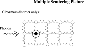
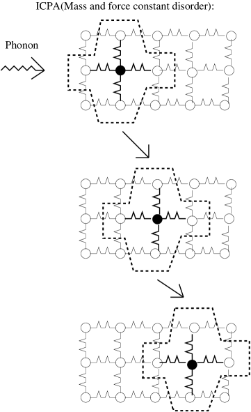
Figure 1: Multiple scattering picture in the CPA(top) and with the ICPA(bottom). The filled circle is the site of the fluctuation, and the contours around it indicate its area of influence. The arrows with the ICPA indicate the itineration of the fluctuation to neighboring sites. The details are given in the text .

The lower three panels in Fig.1 illustrate scattering sites in the ICPA. The difference from the CPA is that the region of influence is not only the site of fluctuation but also its neighboring environment around the fluctuation site. The figure shows an example (dotted contour) where the environment includes nearest neighbors only (The calculations could be extended to further neighbors as well). When the phonon interacts with the fluctuation site in the top panel of the three, it scatters also from all of its neighbors since their spring constants also undergo changes (denoted by the thick spring lines in contrast to the thin ones for the average medium). The whole cluster of atoms undergoes fluctuations in force-constants as the occupation of the fluctuation site changes. One has to keep in mind that the force-constant between the fluctuation site and its neighbor on the right, say, depends on the occupation of both sites, as is true for the next neighboring site on its right as well. So, one is led to include the irreducible scatterings by the fluctuation on all neighboring sites, which then requires inclusion of scattering by the fluctuations on its neighbors etc., until the irreducible scatterings extend throughout the entire sample. A simple example of this process is indicated in the middle and bottom panels. Indeed, Mills and Ratanavararakshatca have shown that once there are non-diagonal terms in the scattering, the self-energy must include these migrations (itinerations) of the scatterer throughout the sample in order to attain unitarity and thereby guarantee that the average Green’s function will be properly analytic or Herglotz. The self-consistent scattering and the resulting coherent potential about a single defect thus itinerates from defect to defect throughout the sample, making it an itinerant coherent potential. The scattering could have started from any site in the sample so that the result is also fully translationally invariant, and the self-energy is $q$-dependent but diagonal in the $q$-space of the Brillouin zone of the underlying periodic lattice structure. Fig. 2(b) illustrates a typical self-energy diagram in the ICPA. The solid and dotted overlapping ellipses denote the multiple scattering by a single-site and its neighbors, i.e. by a cluster of atoms, and the subsequent itineration of this process. The thin dotted lines and the thick double lines are as in Fig.2(a).

Figure 2: The self-energy diagrams in the CPA(top) and a typical example in the ICPA(bottom). The details are given in the text .

In the multiple scattering framework, we calculate the self-energy ${\bf\Sigma}\left(\omega^{2}\right)$, defined by

$$\ll{\bf G}\left(\omega^{2}\right)\gg=[{\bf G}_{vca}^{-1}\left(\omega^{2}\right)-{\bf{\Sigma}}\left(\omega^{2}\right)]^{-1},$$ (20)

where ${\bf G}_{vca}$ is the unperturbed Green’s function,

$${\bf G}_{vca}=\left(\overline{\bf m}\omega^{2}-{\overline{\bf{\Phi}}}\right)^{-1},$$ (21)

and ${\overline{\bf m}}$ and ${\overline{\bf{\Phi}}}$ are the configuration-averaged mass and force-constant operators respectively.

Our major task is to calculate the self-energy ${\bf{\Sigma}}\left(\omega^{2}\right)$. Let us consider $\widehat{\bf K}=\left(\widehat{\bf m}\omega^{2}-\widehat{\bf\Phi}\right)=\widehat{\bf G}^{-1}$. Using the 2$\times$2 block representation of augmented-space operators of Eq.(12) we get

$$\widehat{\bf G}=\left(\begin{array}[]{cc}\overline{\bf G}&{\bf G}^{\prime}\\ {{\bf G}^{\prime}}^{\dagger}&\widetilde{\bf G}\end{array}\right)=\left(\begin{array}[]{cc}\overline{\bf K}&{\bf K}^{\prime}\\ {{\bf K}^{\prime}}^{\dagger}&\widetilde{\bf K}\end{array}\right)^{-1}.$$ (22)

Using the relation for the inverse of an operator in 2$\times$2 block form mat , namely,

$${\hat{\bf A}}^{-1}=\left(\begin{array}[]{cc}\left(\bar{\bf A}-{\bf A}^{\prime}{\widetilde{\bf A}}^{-1}{\bf A}^{\prime\dagger}\right)^{-1}&-\left(\widetilde{\bf A}{{\bf A}^{\prime}}^{-1}\bar{\bf A}-{\bf A}^{\prime\dagger}\right)^{-1}\\ -\left(\bar{\bf A}{{\bf A}^{\prime\dagger}}^{-1}\widetilde{\bf A}-{\bf A}^{\prime}\right)^{-1}&\left(\widetilde{\bf A}-{\bf A}^{\prime\dagger}{\bar{\bf A}}^{-1}{\bf A}^{\prime}\right)^{-1}\end{array}\right),$$ (23)

we get

$$\overline{\bf G} = [\left(\overline{\bf m}\omega^{2}-\overline{\bf\Phi}\right)-{\bf K}^{\prime}\left(\widetilde{\bf m}\omega^{2}-\widetilde{\bf\Phi}\right)^{-1}{\bf K}^{\prime\dagger}]^{-1}$$ (24)

$$= [{\bf G}_{vca}^{-1}-{\bf K}^{\prime}\{{\bf G}_{vca}^{-1}-[\left(\overline{\bf m}\omega^{2}-\overline{\bf\Phi}\right)-$$

$$\enskip\enskip\enskip\enskip\enskip\enskip\left(\widetilde{\bf m}\omega^{2}-\widetilde{\bf\Phi}\right)]\}^{-1}{\bf K}^{\prime\dagger}]^{-1}$$

$$= [{\bf G}_{vca}^{-1}-{\bf K}^{\prime}{\bf F}{\bf K}^{\prime\dagger}]^{-1}.$$

Therefore, the self-energy is given by

$${\bf{\Sigma}}={\bf K}^{\prime}{\bf F}{\bf K}^{\prime\dagger},$$ (25)

where

$${\bf F}=\widetilde{\bf K}^{-1}=\{{\bf G}_{vca}^{-1}\tilde{\bf I}-\widetilde{\bf V}\}^{-1},$$ (26)

and where

$$\widetilde{\bf V}=\left(\overline{m}\tilde{\bf I}-\widetilde{\bf m}\right)\omega^{2}-\left(\bar{\phi}\tilde{\bf I}-\tilde{\bf\Phi}\right).$$ (27)

The quantity $\widetilde{\bf V}$ denotes all perturbations to the average medium, and ${\bf F}$ contains the itineration of the fluctuation in the average medium.

Up to this point, the scattering formalism is exact. We now introduce the ICPA by restricting the states within the configuration space $\Theta-|f\rangle\langle f|$ to the single-fluctuation states, the notation for which is given by Eq.(14). Making the site and cartesian indices explicit, we obtain for ${\bf\Sigma}$ in Eq.(20), under this restriction,

$$\Sigma_{ij}^{\alpha\beta}=\sum K^{(m)}_{\alpha i,\delta k}F^{(m)(n)}_{\delta k,\gamma l}K^{\prime\dagger(n)}_{\gamma l,\beta j}.$$ (28)

The sumations are over the repeated indices, and the fluctuation itinerator ${\bf F}$ is given by a Dyson equation,

$${\bf F}^{(i)(j)}={\bf G}_{vca}[\delta_{(i)(j)}+\sum_{l}\widetilde{\bf V}^{(i)(l)}{\bf F}^{(l)(j)}],$$ (29)

where only the site index of the fluctuation is shown. The quantities in (23) are translationally invariant as follows:

$$K^{(m)}_{ik} = K^{(0)}_{i-m,k-m},$$

$$F^{(m)(n)}_{kl} = F^{(0)(n-m)}_{k-m,l-m}.$$ (30)

The single fluctuation in Eq.(23) can be considered to have been ‘created’ by ${\bf K}^{\prime(n)}$ at site $n$, itinerated to site $m$ by ${\bf F}^{(n)(m)}$ and ‘destroyed’ by ${\bf K}^{\prime\dagger(m)}$ at site $m$. The ${\bf K}$, ${\bf K}^{\prime\dagger}$ and ${\bf F}$ matrices have elements which are non-zero only for site indices within the environment of the appropriate defects i.e. the indices $i$ and $k$ ($l$ and $j$) must be within the neighborhood perturbed by the defect at $m$($n$). The terms with more than one fluctuation(defect) present at a time correspond to coherent pair and ‘defect cluster’ scattering and are neglected in the single-site scattering considered here. All of these operators act in the augmented space. The Equations (20)-(24) define an itinerant single-site multiple scattering theory.

II.3 Self-consistency

The restriction in Eq.(23) to states of $\Theta-|f\rangle\langle f|$ containing only a single fluctuation is a very severe approximation. Multiple-fluctuation states are of course present in ${\bf F}$ and contribute to ${\bf\Sigma}$. In the spirit of the CPA, these are included approximately by introducing self-consistency. As in the CPA klgd ; rmp we obtain self-consistency by replacing ${\bf G}_{vca}$ in ${\bf F}$ in Eq.(24) by a conditional propagator ${\bf G}^{(i)}$, identical to $\overline{\bf G}=\ll{\bf G}\gg$ except that all irreducible scatterings beginning or ending on site $i$ are omitted, so that ${\bf F}$ would then be given by

$${\bf F}^{(i)(j)}={\bf G}^{(i)}[\delta_{(i)(j)}+\sum_{l}\widetilde{\bf V}^{(i)(l)}{\bf F}^{(l)(j)}].$$ (31)

In parallel with Eq.(15), ${\bf G}^{(i)}$ contains a conditional self-energy ${\bf\Sigma}^{(i)}$ which, is like Eq.(23), except that it includes only those scatterings that neither start nor end on $i$,

$${\bf G}^{(i)}=[\left({\bf G}_{vca}\right)^{-1}-{\bf\Sigma}^{(i)}]^{-1},$$ (32)

$${\bf\Sigma}^{(i)}=\sum_{l,m\neq i}{\bf K}^{\prime(l)}{\bf F}^{(l)(m)}{\bf K}^{\prime\dagger(m)}.$$ (33)

Referring to Fig.2a, the double line in the multiple-scattering graphs is the propagator ${\bf G}^{(i)}$ when the solid dot refers to site $i$. We obtain the itinerant CPA by allowing ${\bf K}^{\prime}$,${\bf K}^{\prime\dagger}$, and $\widetilde{\bf V}$ to include force-constant disorder as well and therefore defect itineration in Equations (26)-(28). This closed set of equations defines our single-site, self-consistent, multiple-scattering theory which, when solved, yields ${\bf F}$. Inserting ${\bf F}$ into Eq.(20) for ${\bf\Sigma}$ and the result into Eq.(15) then yields ${\bf G}$. It is already known that Eqs.(15),(20),(26)-(28) have a unique solution which yields a Herglotz average Green’s function klgd . A major difference between this and previous generalizations of the CPA is that for scattering from single-site fluctuations with off-diagonal and/or environmental disorder, as is considered here, the matrix representation of the operator $\widetilde{\bf V}$ has elements which transfer or itinerate the fluctuation from site to site. This feature causes the self-energy to have nonzero off-diagonal elements in real-space extending across the sample and thus contributes importantly to such quantities as the two-particle vertex corrections in a way the CPA cannot chit .

It now remains to solve these equations, making use of the translational symmetry of the augmented-space operators. We accomplish this by Fourier transforms on the fluctuation-site labels,

$$A\left(\vec{q}\right)_{mn}=N^{-1}\sum_{l,l^{\prime}}A_{l+m,l^{\prime}+n}^{(l)(l^{\prime})}e^{-i\vec{q}\cdot\vec{R}_{ll^{\prime}}},$$ (34)

and

$$A^{(l)(l^{\prime})}_{l+m,l^{\prime}+n}=N^{-1}\sum_{\vec{q}}A\left(\vec{q}\right)_{mn}e^{i\vec{q}\cdot\vec{R}_{ll^{\prime}}},$$ (35)

where $\vec{R}_{ll^{\prime}}$ is the lattice vector connecting the fluctuation sites $l$ and $l^{\prime}$, $m$ and $n$ are neighbors of $l$ and $l^{\prime}$ respectively, and the $\vec{q}$ sum is over the Brillouin zone.

We can also effect Fourier transforms on the site indices themselves. That of the self-energy is

$$\Sigma\left(\vec{q}\right)=N^{-1}\sum_{ij}\Sigma_{ij}e^{-\vec{q}\cdot\vec{R}_{ij}}.$$ (36)

From Eqs.(20), (25) and (29),it follows that

$$\Sigma\left(\vec{q}\right)=\sum_{l,m,n,p}K_{lm}^{(0)}F\left(\vec{q}\right)_{mn}K_{np}^{\prime\dagger(0)}e^{-i\vec{q}\cdot\vec{R}_{lp}}.$$ (37)

In this notation, Eq (26) becomes

$$F\left(\vec{q}\right)_{mn}=G_{mn}^{(0)}+\sum_{rp}G_{mr}^{(0)}\widetilde{V}\left(\vec{q}\right)_{rp}F\left(\vec{q}\right)_{pn}.$$ (38)

The cartesian indices here are implicit so that each quantity is a 3$\times$3 matrix .

Since the range of interaction in real-space is finite, the perturbations ${\bf K}^{\prime(i)}$ and $\widetilde{\bf V}\left(\vec{q}\right)$ are finite matrices, nonzero only over a finite set of real sites. For example, if we consider nearest-neighbor perturbation only in a single-site approximation, the $\widetilde{\bf V}\left(\vec{q}\right)$ and ${\bf K}^{\prime}$ are 3$\left(Z+1\right)\times$ 3 $\left(Z+1\right)$ matrices where $Z$ is the number of nearest neighbors. This is the minimum matrix size necessary to exhibit all the impurity modes or states about each fluctuation site.

In full matrix notation, we obtain

$${\bf F}\left(\vec{q}\right)=[{{\bf G}^{(0)}}^{-1}-\widetilde{\bf V}\left(\vec{q}\right)]^{-1}.$$ (39)

These matrices , for example, for an fcc lattice, are of dimension 39$\times$39.

In order to evaluate ${\bf G}^{(0)}$ we rewrite Eq. (27) as,

$${\bf G}^{(0)}=[\left({\bf G}_{vca}\right)^{-1}-{\bf\Sigma}^{(0)}]^{-1}=[\ll{\bf G}\gg^{-1}+\widetilde{\bf\Sigma}^{(0)}]^{-1},$$ (40)

where, $\widetilde{\bf\Sigma}^{(0)}=\left({\bf\Sigma}-{\bf\Sigma}^{(0)}\right)$. The conditional self-energy $\widetilde{\bf\Sigma}^{(0)}$ contains only those scatterings which either start or end with a perturbation caused by a fluctuation at site $0$. Thus, to evaluate the self-consistent propagator ${\bf G}^{(0)}$, we need to know $\ll{\bf G}\gg$. But $\ll{\bf G}\gg$ is obtained from Eq.(15), which becomes

$$\ll G\left(\vec{q}\right)\gg = [G_{vca}\left(\vec{q}\right)^{-1}-\Sigma\left(\vec{q}\right)]^{-1},$$

$$\ll G_{ij}\gg = N^{-1}\sum_{\vec{q}}\ll G\left(\vec{q}\right)\gg e^{-i\vec{q}\cdot\vec{R}_{ij}}.$$ (41)

After reaching self-consistency by the procedure described below, we use these expressions to calculate densities of states and spectral functions.

The conditional self-energy $\widetilde{\bf\Sigma}^{(0)}$ can be broken up into two contributions:

(i) Scattering that starts from a defect at site $0$ and ends at site $j$.

(ii) Scattering that starts at $j$ but ends at $0$.

This decomposition results in

$$\widetilde{\bf\Sigma}^{(0)} = \sum_{j}[{\bf K}^{\prime(0)}{\bf F}^{(0)(j)}{\bf K}^{\prime\dagger(j)}+{\bf K}^{\prime(j)}{\bf F}^{(j)(0)}{\bf K}^{\prime\dagger(0)}]$$ (42)

$$\enskip\enskip\enskip\enskip-{\bf K}^{\prime(0)}{\bf F}^{(0)(0)}{\bf K}^{\prime\dagger(0)}.$$

The last term is subtracted to avoid overcounting when $j$=$0$.

In a block notation similar to that of Eq.(12), we have

$$\widetilde{\bf\Sigma}^{(0)}=\left(\begin{array}[]{cc}{\bf\Sigma}_{1}&{\bf\Sigma}_{3}\\ {\bf\Sigma}^{\dagger}_{3}&0\end{array}\right),$$ (43)

$${\bf G}^{(0)}=\left(\begin{array}[]{cc}{\bf G}^{(0)}_{1}&{\bf G}^{(0)}_{3}\\ {\bf G}^{\dagger(0)}_{3}&{\bf G}^{(0)}_{2}\end{array}\right),$$ (44)

$$\ll{\bf G}\gg=\left(\begin{array}[]{cc}{\bf G}_{1}&{\bf G}_{3}\\ {\bf G}^{\dagger}_{3}&{\bf G}_{2}\end{array}\right).$$ (45)

where, for a genaral operator $\hat{\bf A}$, ${\bf A}_{1}$ begins and ends with scattering about site $0$ , ${\bf A}_{2}$ neither begins nor ends with scattering about site $0$ and ${\bf A}_{3}({\bf A}_{3}^{\dagger})$ begins(ends) with scattering at the site $0$ and ends(begins) with scattering about a site different from $0$. The term ${\bf\Sigma}_{2}$ is $0$ since $\widetilde{\bf\Sigma}^{(0)}$ must begin or end at the site $0$. From Eq. (35), we have

$${\bf G}^{(0)}=\ll{\bf G}\gg\left({\bf I}+\widetilde{\bf\Sigma}^{(0)}\ll{\bf G}\gg\right)^{-1},$$ (46)

which leads to

$${\bf G}_{1}^{(0)} = \overline{\bf X}[{\bf I}+\left({\bf\Sigma}_{1}-{\bf\Sigma}_{3}{\bf G}_{2}{\bf\Sigma}^{\dagger}_{3}\right)\overline{\bf X}+{\bf\Sigma}_{3}{\bf G}^{\dagger}_{3}]^{-1},$$ (47)

where

$$\overline{\bf X}=\left({\bf I}+{\bf G}_{3}{\bf\Sigma}^{\dagger}_{3}\right)^{-1}{\bf G}_{1}.$$ (48)

after a lengthy algebraic analysis which was previously given in Ref.18.

In order to evaluate these expressions klgd , we need to calculate four terms: ${\bf G}_{1}$,${\bf\Sigma}_{1}$, ${\bf G}_{3}{\bf\Sigma}^{\dagger}_{3}$ and ${\bf\Sigma}_{3}{\bf G}_{2}{\bf\Sigma}^{\dagger}_{3}$. The first term ${\bf\Sigma}_{1}$ is just a finite sum of finite matrices and can be evaluated directly, but the other two terms involve sums which range over all sites in the solid and must be evaluated by Fourier transforms. This is done in the following way,

$$\left(G_{3}\Sigma^{\dagger}_{3}\right)_{t,t^{\prime}} = \sum_{m}\sum_{r,n,l}\ll G\left(\omega^{2}\right)\gg_{t,m+r}K^{\prime(m)}_{m+r,m+n}$$

$$\times F^{(m)(0)}_{m+n,l}K^{\prime\dagger(0)}_{l,t^{\prime}}-\sum_{r}\ll G\left(\omega^{2}\right)\gg_{t,r}\widetilde{\Sigma}^{(0)}_{r,t^{\prime}},$$

which becomes

$$\left(G_{3}\Sigma^{\dagger}_{3}\right)_{t,t^{\prime}} = \frac{1}{N}\sum_{\vec{q}}\sum_{r}\ll G\left(\vec{q}\right)\gg e^{i\vec{q}\cdot\vec{R}_{tr}}M\left(\vec{q}\right)_{r,t^{\prime}}$$ (49)

$$\text{\hskip 56.9055pt}-\left(G_{1}\Sigma_{1}\right)_{t,t^{\prime}},$$

and,similarly,

$$\left(\Sigma_{3}G_{2}\Sigma^{\dagger}_{3}\right)_{t,t^{\prime}} = \frac{1}{N}\sum_{\vec{q},r,r^{\prime}}M\left(\vec{q}\right)_{tr}\ll G\left(\vec{q}\right)\gg e^{i\vec{q}\cdot\vec{R}_{rr^{\prime}}}M\left(\vec{q}\right)_{r^{\prime},t^{\prime}}$$ (50)

$$-(\Sigma_{1}G_{1}\Sigma_{1}+\Sigma_{1}G_{3}\Sigma^{\dagger}_{3}+\Sigma_{3}G^{\dagger}_{3}\Sigma_{1})_{t,t^{\prime}},$$

where

$$M\left(\vec{q}\right)_{r,t^{\prime}}=\sum_{nl}K^{\prime(0)}_{rn}F\left(\vec{q}\right)_{nl}K^{\prime\dagger(0)}_{lt^{\prime}}.$$ (51)

In these equations, $0$ is the index of the single fluctuation-site in consideration; $r,r^{\prime},t,t^{\prime},l,n$ are the neighboring sites of $0$; and $m,m^{\prime}$ are general sites in the sample. So, it is clear that one needs to work only on matrices of size 3$\left(Z+1\right)\times$3 $\left(Z+1\right)$ and use the Fourier transform of operators to handle the itineration of the fluctuation throughout the entire sample. An interesting point to note is that the quantities $G_{3}\Sigma_{3}^{\dagger}$ and $\Sigma_{3}G_{2}\Sigma_{3}^{\dagger}$ represent the scattering and itineration of the disturbance including the effect of the off-diagonal and environmental disorder. In case of diagonal-disorder only, they vanish giving ${\bf G}_{1}^{(0)}={\bf G}_{1}\left({\bf I}+{\bf\Sigma}_{1}\right)^{-1}$, which is the CPA self-consistent propagator, and the self-consistent set of equations reduces to the CPA equations.

The inputs to the self-consistency cycle are ${\bf G}^{(0)}_{start}={\bf G}_{vca}$(or some better guess) , ${\bf K}^{\prime},{\bf K}^{\prime\dagger}$ and $\widetilde{\bf V}\left(\vec{q}\right)$. The procedures for evaluating the latter three quantities are given in the Appendix. The cycle consists of the following steps :

1. calculation of ${\bf F}\left(\vec{q}\right)$ using Eqs.(33) and (34).

2. calculation of $\Sigma\left(\vec{q}\right)$ using Eq.(32).

3. calculation of $\ll G\left(\vec{q}\right)\gg$ and $\ll G\left(\omega^{2}\right)\gg$ using Eq.(36).

4. calculation of ${\bf G}_{1}^{(0)}$ using Eqs.(42),(43),(44) and (45)

5. If the results of steps 1.-4. are acceptably close to those of the previous cycle, stop. If not, use as input to step 1 and iterate.

The iterations are done till self-consistency is achieved for each $\vec{q}$-point in the Brillouin zone. In the process of achieving self-consistency, one calculates $\ll G\gg$ in both real-space and in $\vec{q}$-space; each is needed to obtain densities of states and spectral densities respectively. In the next section, we describe how these are used to calculate physical quantities of interest and discuss their significance.

III Important quantities; sum rules

In this section we derive results for important physical quantities such as the densities of states (partial and total), spectral densities (partial and total) and inelastic scattering cross sections (coherent and incoherent). All of these are derivable from the real-space and the $\vec{q}$-space configuration-averaged Green’s function and enable us to make direct comparisons with experimental measurements.

III.1 Densities of states

The total density of states for a 3-dimensional system is defined as,

$$\nu\left(\omega\right)=\frac{1}{3\pi N}{\cal I}m\{Tr\ll{\bf mG}(\omega^{2})\gg\},$$ (52)

where ${\bf m}$ is the mass matrix, and $N$ is the number of sites. In augmented space we have,

$$\ll mG\gg_{ii} = \langle if|\widehat{\bf m}\widehat{\bf G}|if\rangle,$$ (53)

$$= \langle if|\widehat{\bf m}|if\rangle\langle if|\widehat{\bf G}|if\rangle$$

$$+\langle if|\widehat{\bf m}|if_{i}\rangle\langle if_{i}|\widehat{\bf G}|if\rangle,$$

$$= \overline{m}\overline{G}_{00}+m^{\prime}\langle if_{i}|\widehat{\bf G}|if\rangle.$$

To evaluate the second term, we use the notation of Eq.(12) for the operators $\widehat{\bf G}$ and $\widehat{\bf K}=\widehat{\bf G}^{-1}$. Then, using Eq.(18), we obtain

$$\langle if_{i}|\widehat{\bf G}|if\rangle={\bf G}^{\prime\dagger}=-\widetilde{\bf K}^{-1}{\bf K}^{\prime\dagger}\overline{\bf G}=-{\bf FK}^{\prime\dagger}\overline{\bf G}.$$ (54)

We can, therefore, write

$$\langle if_{i}|\widehat{\bf G}|if\rangle=-\sum_{l}\sum_{j,n}F_{ij}^{(i)(l)}K_{jn}^{\prime\dagger(l)}\ll G\gg_{ni}.$$

Fourier transforming over the fluctuation site according to (29) gives

$$\langle if_{i}|\widehat{G}|if\rangle = -\frac{1}{N}\sum_{l,j,n}\sum_{\vec{q}}F\left(\vec{q}\right)_{0,j-l}e^{i\vec{q}\cdot\vec{R}_{il}}$$

$$\text{\hskip 56.9055pt}\times K^{\prime\dagger}_{j-l,n-l}\ll G\gg_{ni}.$$

The Fourier transform of $\ll{\bf G}\gg$ on the real-site index now gives,

$$\langle if_{i}|\widehat{G}|if\rangle = -\frac{1}{N^{2}}\sum_{l,j,n}\sum_{\vec{q}\vec{q^{\prime}}}F\left(\vec{q}\right)_{0,j-l}e^{i\vec{q}\cdot\vec{R}_{il}}$$

$$\text{\hskip 56.9055pt}\times K^{\prime\dagger}_{j-l,n-l}\ll G(\vec{q^{\prime}})\gg e^{i\vec{q}\cdot\vec{R}_{ni}}.$$

Finally we obtain,

$$\langle if_{i}|\widehat{\bf G}|if\rangle = -\sum_{mp}\sum_{\vec{q}}F\left(\vec{q}\right)_{0,m}K^{\prime\dagger}_{mp}e^{i\vec{q}\cdot\vec{R}_{p}}\ll G(\vec{q})\gg,$$

where, $m=j-l$, $p=n-l$, the neighboring sites perturbed by the fluctuation. All the terms on the right hand side have been calculated already in the process of achieving self-consistency. The evaluation of the average density of states is thus straightforward.

The partial density of states for atoms of type $s$ is given by

$$\nu\left(\omega\right)_{s}=\frac{m_{s}}{3\pi N}{\cal I}m\{Tr\ll G(\omega^{2})^{ss}\gg_{ii}\},$$ (55)

where

$$\ll G^{ss}\gg_{ii}=\ll G^{ss}\gg_{00}=\langle 0f|\widehat{\bf\eta}_{0}^{s}\widehat{\bf G}|0f\rangle$$ (56)

because of translation invariance. We thus have

$$\ll G^{s}\gg_{0}=\ll G^{ss}\gg_{00} = \langle 0f|\widehat{\bf\eta}^{s}_{0}|0f\rangle\langle 0f|\widehat{\bf G}|0f\rangle$$ (57)

$$+ \langle if|\widehat{\bf\eta}^{s}_{0}|0f_{0}\rangle\langle 0f_{0}|\widehat{\bf G}|0f\rangle,$$

and, from Eq. (11), it follows that

$$\nu\left(\omega\right)_{A} = -\frac{m_{A}}{3\pi}{\cal I}m[c_{A}\{\langle 0f|\widehat{\bf G}|0f\rangle\}$$

$$\enskip+\sqrt{c_{A}c_{B}}\{\langle 0f_{0}|\widehat{\bf G}|0f\rangle\}],$$

$$\nu\left(\omega\right)_{B} = -\frac{m_{B}}{3\pi}{\cal I}m[c_{B}\{\langle 0f|\widehat{\bf G}|0f\rangle\}$$

$$\enskip-\sqrt{c_{A}c_{B}}\{\langle 0f_{0}|\widehat{\bf G}|0f\rangle\}].$$

The elements of $\widehat{\bf G}$ in Eq.(53) were already evaluated while calculating the average density of states above.

The partial Green’s functions $\ll G^{s}\gg_{0}$ are used in calculating the incoherent scattering structure factor which is directly measured in the experiments,

$$\ll S_{incoh}\left(\vec{Q},\omega\right)\gg=\sum_{s}b^{2}_{s}\vec{Q}\cdot{\cal I}m\ll G^{s}\left(\omega\right)\gg_{0}\cdot\vec{Q},$$ (59)

where $b_{s}$ is the incoherent scattering length for atoms of type $s$, and $Q$ is the phonon wavenumber.

III.2 Spectral densities

The average spectral function is defined as,

$$\ll{\cal A}_{\lambda}\left(\vec{q},\omega^{2}\right)\gg=\frac{1}{\pi}{\cal I}m\ll G_{\lambda}\left(\vec{q},\omega^{2}\right)\gg,$$ (60)

where $\lambda$ is a normal-mode branch index. More interesting quantities to calculate are the conditional or partial Green’s functions $\ll G^{ss^{\prime}}\left(\vec{q},\omega^{2}\right)\gg$ in $\vec{q}$-space because these enable one to calculate the coherent-scattering structure factors which are measured directly in the neutron-scattering experiments and are given by,

$$\ll S_{\lambda}\left(\vec{q},\omega\right)\gg_{coh}=\sum_{ss^{\prime}}d_{s}d_{s^{\prime}}\frac{1}{\pi}{\cal I}m\ll G^{ss^{\prime}}_{\lambda}\left(\vec{q},\omega^{2}\right)\gg,$$ (61)

where, $d_{s}$ is the coherent scattering length for the species $s$.

The conditional Green’s functions are defined as

$$\ll G^{ss^{\prime}}\left(\vec{q},\omega^{2}\right)\gg=\frac{1}{N}\sum_{ij}\ll G^{ss^{\prime}}\left(\omega^{2}\right)\gg_{ij}e^{-\vec{q}\cdot\vec{R}_{ij}},$$

$$\ll G^{ss^{\prime}}\left(\omega^{2}\right)\gg_{ij}=\ll\widehat{\bf\eta}^{s}_{i}\widehat{\bf G}\left(\omega^{2}\right)\widehat{\bf\eta}^{s^{\prime}}_{j}\gg=\langle if|\widehat{\bf\eta}^{s}_{i}\widehat{\bf G}\widehat{\bf\eta}^{s^{\prime}}_{j}|jf\rangle$$

$$=\langle if|\widehat{\bf\eta}^{s}_{i}|if\rangle\langle if|\widehat{\bf G}|jf\rangle\langle jf|\widehat{\bf\eta}^{s^{\prime}}_{j}|jf\rangle$$

$$+\langle if|\widehat{\bf\eta}^{s}_{i}|if_{i}\rangle\langle if_{i}|\widehat{\bf G}|jf\rangle\langle jf|\widehat{\bf\eta}^{s^{\prime}}_{j}|jf\rangle$$

$$+\langle if|\widehat{\bf\eta}^{s}_{i}|if\rangle\langle if|\widehat{\bf G}|jf_{j}\rangle\langle jf_{j}|\widehat{\bf\eta}^{s^{\prime}}_{j}|jf\rangle$$

$$+\langle if|\widehat{\bf\eta}^{s}_{i}|if_{i}\rangle\langle if_{i}|\widehat{\bf G}|jf_{j}\rangle\langle jf_{j}|\widehat{\bf\eta}^{s^{\prime}}_{j}|jf\rangle.$$ (62)

In Eq.(57) the index $\lambda$ is to be understood. These four terms include all the possible scattering processes when two different sites are occupied by two species. The four different terms involve calculations of the Green’s function under various circumstances of coupling between the average and the fluctuation states weighted by the appropriate concentrations .

We obtain from (57)

$$\ll G^{ss^{\prime}}\gg_{ij} = c_{s}c_{s^{\prime}}\langle if|\widehat{\bf G}|jf\rangle+[c_{s^{\prime}}\sqrt{c_{s}(1-c_{s})}$$ (63)

$$\times \left(-1\right)^{(1-n^{s})}\langle if_{i}|\widehat{\bf G}|jf\rangle]+[c_{s}\sqrt{c_{s^{\prime}}(1-c_{s^{\prime}})}$$

$$\times \left(-1\right)^{(1-n^{s^{\prime}})}\langle if|\widehat{\bf G}|jf_{j}\rangle]+c_{s}c_{s^{\prime}}$$

$$\text{\hskip 28.45274pt}\times\left(-1\right)^{(n^{s}+n^{s^{\prime}})}\langle if_{i}|\widehat{\bf G}|jf_{j}\rangle.$$

The integer $n^{s}$ is equal to 1 if $s$=A and is equal to 0 if $s$=B.

These terms can be easily calculated using Fourier transforms as has been previously demonstrated for the density of states. The final forms of the conditional Green’s functions in $\vec{q}$-space are

$$\ll G^{AA}\left(\vec{q},\omega^{2}\right)\gg = c_{A}^{2}\ll G\left(\vec{q},\omega^{2}\right)\gg+c_{A}\sqrt{c_{A}c_{B}}(T_{1}+$$

$$\enskip\enskip\enskip T_{2})+c_{A}c_{B}T_{3},$$

$$\ll G^{BB}\left(\vec{q},\omega^{2}\right)\gg = c_{B}^{2}\ll G\left(\vec{q},\omega^{2}\right)\gg-c_{B}\sqrt{c_{A}c_{B}}(T_{1}+$$

$$\enskip\enskip\enskip T_{2})+c_{A}c_{B}T_{3},$$

$$\ll G^{AB}\left(\vec{q},\omega^{2}\right)\gg = c_{A}c_{B}\ll G\left(\vec{q},\omega^{2}\right)\gg+\sqrt{c_{A}c_{B}}(c_{B}T_{1}$$

$$\enskip\enskip\enskip-c_{A}T_{2})-c_{A}c_{B}T_{3},$$

$$\ll G^{BA}\left(\vec{q},\omega^{2}\right)\gg = c_{A}c_{B}\ll G\left(\vec{q},\omega^{2}\right)\gg-\sqrt{c_{A}c_{B}}(c_{A}T_{1}$$ (64)

$$\enskip\enskip\enskip-c_{B}T_{2})-c_{A}c_{B}T_{3},$$

where

$$T_{1} = \sum_{nm}F_{0n}\left(\vec{q}\right)K^{\prime\dagger}_{nm}e^{i\vec{q}\cdot\vec{R}_{m}}\ll G\left(\vec{q},\omega^{2}\right)\gg,$$

$$T_{2} = \sum_{nm}\ll G\left(\vec{q},\omega^{2}\right)\gg e^{-i\vec{q}\cdot\vec{R}_{n}}K^{\prime}_{nm}F_{m0}\left(\vec{q}\right),$$

$$T_{3} = F_{00}\left(\vec{q}\right)+\sum_{nm}\sum_{lp}F_{0n}\left(\vec{q}\right)K^{\prime\dagger}_{nm}e^{i\vec{q}\cdot\vec{R}_{m}}$$ (65)

$$\text{\hskip 14.22636pt}\times\ll G\left(\vec{q},\omega^{2}\right)\gg e^{-i\vec{q}\cdot\vec{R}_{l}}K^{\prime}_{lp}F_{p0}\left(\vec{q}\right),$$

and where $n,m,l$ and $p$ are the neighboring sites of the fluctuation site $0$ influenced by the perturbation. For the lattices with each site having inversion symmetry, $T_{1}$=$T_{2}$ holds because $T_{1}$ and $T_{2}$ are the contributions from two processes which are conjugate to one another. In that case, $\ll G^{AB}\left(\vec{q},\omega^{2}\right)\gg$= $\ll G^{BA}\left(\vec{q},\omega^{2}\right)\gg$ when $c_{A}$=$c_{B}$.

The sum rules for the conditional Green’s functions are derived the following way: Integrate $\omega\enskip\widehat{\bf G}\left(\omega^{2}\right)$, Eq.(2), along the real axis, closing the contour above at infinity, obtaining

$$\oint d\omega\enskip\omega\enskip\widehat{\bf G}\left(\omega^{2}\right) = \widehat{\bf m}^{-1}\pi i,$$

or

$$\int_{0}^{\infty}d\omega\enskip 2\omega\enskip{\cal I}m\widehat{\bf G}\left(\omega^{2}\right) = \widehat{\bf m}^{-1}\pi.$$ (66)

Similarly, using Eq.(57), taking the Fourier transform of Eq.(58), carrying out the contour integral and inserting (61) yields the sum rule for the partial spectral functions

$$\int_{0}^{\infty}d\omega\enskip 2\omega\enskip{\cal I}m\enskip\ll G^{ss^{\prime}}\left(\vec{q},\omega^{2}\right)\gg=\pi\frac{c_{s}}{m_{s}}\delta_{ss^{\prime}}.$$ (67)

For the total Green’s function we obtain

$$\int_{0}^{\infty}d\omega\enskip 2\omega\enskip{\cal I}m\enskip\ll G\left(\vec{q},\omega^{2}\right)\gg=\pi\left(\frac{c_{A}}{m_{A}}+\frac{c_{B}}{m_{B}}\right).$$ (68)

The experimental dispersion curves are obtained from the wave-vector dependence of the peak frequencies of the structure factors as measured, after a deconvolution of the experimental resolution function. The question is whether the dispersion curves so obtained, which incorporate the effect of the coherent scattering lengths, differ significantly from those obtained from the peak frequencies of the Green’s function itself which gives, in principle, a proper description of the dynamics but does not contain the scattering length weighting. To answer that question one needs to recognize that the peak positions in ${\cal I}m{\bf G}$ are very closely related to the zeroes of ${\cal R}e{\bf G}^{-1}$ at a given wave vector. If we diagonalize the Hermitian ${\cal R}e{\bf G}^{-1}$ both with respect to mode and species index, each of the two species components of ${\cal R}e{\bf G}^{-1}$ will have a zero. Correspondingly, each of the two components of ${\cal I}m{\bf G}$ will have a peak, if ${\cal I}m{\bf\Sigma}$ does not wipe it out. So, in the species representation, the different matrix elements ${\cal I}mG^{ss^{\prime}}$ will thus all have these peaks at nearly the same frequencies. Thus, the weighting of the $G^{ss^{\prime}}$ by the scattering lengths will not shift the peak positions significantly even when the scattering lengths differ appreciably. The intensities and the lineshapes of $S_{coh}$ and ${\cal I}m{\bf G}$ may differ significantly, but the peak positions will generally differ little. In summary, the structure factor fairly accurately reflects the phonon dynamics contained in ${\bf G}$ with regard to the dispersion curves, an important fact illustrated below in the next two sections where we present our calculations on Ni₅₅Pd₄₅ and Ni₅₀Pt₅₀ alloys.

IV Application to Ni₅₅Pd₄₅; weak force-constant disorder

In the next two sections we explore the relative importance of force-constant disorder and mass disorder for the vibrational properties of random alloys in two specific alloys Ni₅₅Pd₄₅ and Ni₅₀Pt₅₀. In the former alloy, the mass disorder is much larger than the force-constant disorder. The mass ratio $m_{Pd}/m_{Ni}$ is 1.812, whereas the Pd force-constants are only about 15$\%$ larger than those of Ni dbm ; bvk . In the latter alloy, both the mass disorder and the force-constant disorder are large, providing an interesting contrast between the two materials. For both the cases we have done our calculations on 200 $\omega$-points and have used a small imaginary frequency part of -0.01 in the Green’s function. For the Brillouin zone integration 356 ${\vec{q}}$-points in the irreducible 1/48-th of the zone produced well converged results. The simplest linear-mixing scheme was used to accelerate the convergence. For both the cases the number of iterations ranged from 3 to 13 depending on the frequency $\omega$.

For Ni₅₅Pd₄₅, we compare the results of virtual crystal(VCA), CPA, and ICPA computations, using the ICPA force-constants to construct the averages used in the VCA and CPA and compare the results with experiment. We make a distinction between that use of the VCA and of ‘mean crystal’ models in which the average mass is employed and a set of ‘mean-crystal’ force-constants are fitted as parameters to the experimental data.

Kamitakahara and Brockhouse expt2 investigated Ni₅₅Pd₄₅ by inelastic neutron scattering and reported a strange observation. A theoretical calulation based on a mean crystal model having the average mass and fitted force-constants between those of Ni and Pd agreed closely with the experimental dispersion curves. This was quite a puzzle because it suggested that the large mass disorder had little effect. There were theoretical studies on this system using recursionmook1 and the average t-matrix approximation kt , but no theoretical results for the frequencies were available. In an attempt to solve this puzzle, we have carried out calculations with the CPA, the ICPA, and the VCA, as well as with the mean-crystal model used in Ref. 3 .

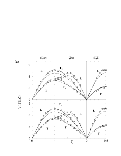
Figure 3: (a)(Top panel)Dispersion curves (frequency $\nu$ vs. reduced wave-vector $\zeta$) for Ni₅₅Pd₄₅ calculated in the ICPA(solid line) and in the VCA(dashed line). The circles are the experimental data expt2 . (Bottom panel) Dispersion curves for Ni₅₅Pd₄₅ calculated in the CPA(solid line) and in the VCA(dashed line). The force-constants used are given in the text. The circles are the experimental data expt2 . (b) Dispersion curves for Ni₅₅Pd₄₅ calculated in the CPA(solid line) and in the mean-crystal model(dashed line) using the force-constants of Ref. 3. The circles are the experimental data expt2 .

For the ICPA calculation, we assumed that the explicit scattering caused by the force-constant disorder was confined to the nearest-neighbors. This assumption is justified because the nearest-neighbor force-constants are an order of magnitude larger than those of the further neighbors so that the nearest-neighbors feel the effect of disorder most strongly. For the virtual-crystal or the average medium into which the scattering was embedded, we kept terms in the Hamiltonian up to the fourth neighbor, which turned out to be sufficient. The problem with force-constant disorder scattering calculations is the general absence of prior information about species-dependent force-constants. We note that Pd is the larger atom here. In the alloy, the Ni-Pd separation is larger than the Ni-Ni separation. As a result, the Ni-Pd force-constants should be less than the Ni-Ni ones. Using this intuitive argument and for simplicity in this illustration, we kept the $\phi_{Ni-Ni}^{\alpha\beta}$ and $\phi_{Pd-Pd}^{\alpha\beta}$ the same as those of the pure materials dbm and reduced the $\phi_{Ni-Pd}^{\alpha\beta}$ below the $\phi_{Ni-Ni}^{\alpha\beta}$ by an $\alpha\beta$ independent factor. The dispersion curves were obtained from the ICPA calculations using $\phi_{Ni-Pd}^{\alpha\beta}$=0.7$\phi_{Ni-Ni}^{\alpha\beta}$ (solid lines) for the nearest neighbors and using the force-constants of Ref.3 for the higher neighbors. They are compared in the top panel of Fig.3(a) with the experimental results expt2 (open circles) and the VCA for the same force-constants(dashed lines). These ICPA dispersion curves were constructed by numerically determining the peaks in the coherent scattering structure factor $\ll S_{\lambda}\left(\vec{q},\omega\right)\gg_{coh}$ given by Eq.(56), which was calculated using the partial spectral functions of Eqs.(59) and (60) and weighting them with the coherent scattering lengths for Ni and Pd. We could thus make a direct comparison with the experimental results because the neutron data observed in the experiments inherently incorporates the effect of the scattering lengths of the species.

Figure 4: (a)Partial and total spectral functions calculated in the ICPA for various $\zeta$ values in the [$\zeta$,0,0] direction in Ni₅₅Pd₄₅. (b) Partial and total structure factors calculated in the ICPA for various $\zeta$ values in the [$\zeta$,0,0] direction in Ni₅₅Pd₄₅. The solid lines are the total contribution, the dotted lines are the Ni-Ni spectra, the long-dashed lines are the Pd-Pd spectra and the dot-dashed lines are the Ni-Pd contributions. The details are given in the text. The left(right) column is for longitudinal(transverse) modes.

Excellent agreement of the ICPA with experiment was obtained for all three symmetry directions and for each branch by varying only one parameter in the force-constant matrix. This suggests that the force-constant disorder is weak and the system is dominated by the mass-disorder, as one would expect from the numerical values of the parameters. It is confirmed by the results of the CPA calculations shown in the bottom panel of the Fig. 3(a), using the same force-constants. As in the top panel, the solid lines are the CPA results, the circles are the experimental points, and the dashed lines are the VCA results. The agreement with the experiment again suggests the dominance of the mass-disorder, but there are more interesting points to note. In the long-wavelength (low $\vec{q}$) regime, the VCA, the CPA, and the ICPA curves are indistinguishable because the self-averaging of both mass and force-constants over a single wavelength reduces both the CPA and the ICPA to the VCA. But, as we move to high wave-vectors , the VCA deviates to frequencies below the experimentally observed ones. This fact is due to the use of an average mass in the Hamiltonian. In the high-wave-vector region, the lighter atoms, i.e. Ni in this case, dominate and push the frequencies up. That is why the CPA and the ICPA agree very well across the Brillouin zone while the VCA fails for the high wave-vectors. The reason that Kamitakahara and Brockhouse got a very good fit to the experimental points in Ref. 3 by using their mean-crystal model is that they obtained parametrized force-constants which were higher than those calculated in the VCA. Though they had used the average mass in their calculations the higher values of the force-constants (They used $\overline{\bf\Phi}=c_{A}{\bf\Phi}_{AA}+c_{B}{\bf\Phi}_{BB}$ rather than $\overline{\bf\Phi}=c_{AA}^{2}{\bf\Phi}_{AA}+c_{BB}^{2}{\bf\Phi}_{BB}+2c_{A}c_{B}{\bf\Phi}_{AB}$) compensated for their omission of the effect of the mass fluctuations. This is illustrated in Fig.3(b). There, the dashed lines are their mean-crystal model calculations, the circles are the experimental points, and the solid lines represent a CPA calculation with the force-constants used in Ref. 3. Here we see that the CPA yields frequencies that are too high in the large wave-vector region. The CPA captures the effect of mass-fluctuation and the domination of the Ni atoms for higher wave-vectors, but the higher values of the assumed mean force-constants pushes the frequencies up further, thereby worsening the agreement with the experiment. But, there was yet another puzzle to solve. Another striking feature is that in spite of incorporating the scattering lengths in our calculations in determining the frequencies there was little change in the ICPA results with respect to the CPA results even though the coherent scattering lengths of Ni and Pd differ significantly( The coherent scattering length for Ni is 1.03 while that of Pd is 0.6). This lack of change can be understood from a comparison between the partial and total spectral functions (Fig. 4(a)) and the partial and the total coherent structure factors (Fig 4(b)). In these figures, we have shown examples of ICPA spectral functions and structure factors along the [$\zeta$,0,0] direction, $\zeta=\frac{|\vec{q}|}{|\vec{q}_{max}|}$, for a low $\zeta$ , one in the middle of the Brillouin zone and one at the edge of the Brilluoin zone. In Fig. 5(a), the solid lines are the total spectral function while the dotted lines are the Ni-Ni spectra, the long-dashed lines are the Pd-Pd spectra and the dot-dashed lines are the Ni-Pd contribution. In each case, the peaks corresponding to the dominating species and that in the Ni-Pd curves occur at the same general positions. For example, in the [.3,0,0]-L curves, the peak in the spectral function is mostly that of Pd atoms while for the [.5,0,0]-L and [1,0,0]-L curves, the contributions are from Ni atoms, the Pd-Pd contribution here is much less and that too is almost completely neutralised by the Ni-Pd contribution in the low frequency region. The occurence of the peaks of the Ni-Pd spectral functions and that of the Ni-Ni or Pd-Pd spectral functions almost at the same position across the Brillouin zone suggests that the inclusion of scattering lengths would primarily alter the relative weights of various contributions and thereby altering only the line shapes, while the dispersion curves wouldn’t undergo significant change. This is demonstrated in Fig. 4(b). There, the solid lines are the coherent structure factors $\ll S_{\lambda}\left(\vec{q},\omega\right)\gg$, the dotted lines are the Ni-Ni spectral functions weighted using the scattering length of Ni, the long-dashed lines are the Pd-Pd spectral functions weighted using the scattering length of Pd and the dot-dashed lines are the Ni-Pd spectral functions weighted by the scattering lengths of Ni and Pd according to Eq.(56). One can see that the weighting affects primarily the peak heights. These explicit numerical results confirm the qualitative argument given at the end of section III.

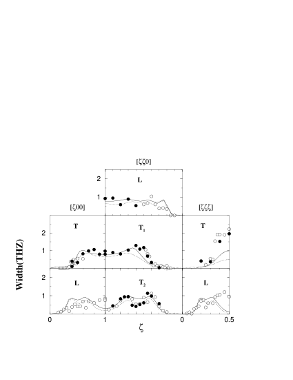
Figure 5: Disorder-induced FWHM’s in Ni₅₅Pd₄₅ calculated in the ICPA(solid line) and in the CPA(dotted line) using the force-constants of Fig. 3(a). The circles are the widths extracted from the experimental results expt2 . The filled circles had better experimental resolution.

The disorder-induced widths are important because the effect of disorder is often manifested in them more directly than in the frequencies. Kamitakahara and Brockhouse extracted full widths at half maxima(FWHM) from their neutron groups by assuming that the observed line shape could be adequately approximated by the convolution of a Gaussian resolution function(representing the experimental resolution) with a Lorentzian natural line shape. Thus, for a comparison of our results with theirs, we have fitted our structure factors to a Lorentzian to extract the widths. The results are shown in Fig.5. The solid lines are the widths (FWHM) obtained in the ICPA, and the dotted lines are those obtained in the CPA. The circles are the experimental points, the filled circles having better resolution expt2 were those in which Kamitakahara and Brockhouse had more confidence. Generally, there is little difference between the widths obtained in the CPA and the ones obtained in the ICPA. In all three symmetry directions and for all branches, the ICPA performs slightly better than the CPA for high wave-vectors. The worst agreement with the experiment is for high wave-vectors in the $[\zeta,0,0]$ and $[\zeta,\zeta,\zeta]$ longitudinal branches and the $[\zeta,\zeta,\zeta]$ transverse branch. In these cases, the low values of the widths in the theoretical calculations can be understood from the shape of the structure factors. From the examples in Fig.4 one can see that the agreement with experiment is good when we have a symmetric line shape, for example, for the [.5,0,0]L mode. On the other hand, the worst agreements with the experimental widths are for cases where we obtain a highly asymmetric line shape, for example, for the [1,0,0]L mode. Fitting Lorentzians to such asymmetric line shapes is not condusive to meaningful values of the FWHMs. Because they obtain higher widths than the theories in those particular cases where the observations have been made with worse resolution(open circles in Fig.5), it is also not clear how trustworthy their treatment of the resolution function is.

The discussion above clearly tells us that for Ni₅₅Pd₄₅, the dominant effect is mass disorder. That alloy therefore does not provide a proper test of the ICPA. Nevertheless, our discussions show how a mean-crystal model can compensate for the neglect of mass fluctuations in alloys with little force-constant disorder through the introduction of erroneous mean force-constants, a classic case of cancellation of errors.

V Ni₅₀Pt₅₀; strong mass and force-constant disorder

The mass ratio $m_{Pt}/m_{Ni}$ is 3, quite large compared to that in the NiPd system. The force-constants of Pt are, on an average, 55$\%$ larger dbm than those of Ni. This makes it a potential example of strong force-constant disorder. Tsunoda et al.expt3 investigated Ni_xPt_1-x by inelastic neutron scattering and compared their observations with the CPA. Here, for illustration, we have considered $x$=0.5 only because that makes it a concentrated alloy and the failure of CPA was, qualitatively, very prominent at this concentration. They compared their incoherent scattering data with that of the CPA which predicted a split band separating out Ni and Pt contributions with a gap between them. The experiments did not reveal a split-band, and it was very clear that the inter-species forces play a significant role. We performed calculations with the CPA and the ICPA. As before, we used the ICPA force-constants in the CPA. The choice of ICPA force-constants was more difficult than for the NiPd because of the larger size difference between Ni and Pt. In this alloy, the Ni-Pt separation is also larger than the Ni-Ni separation. As a result, the Ni-Pt force-constants should also be less than those of Ni-Ni. Moreover, a pair of Ni atoms would find themselves in a cage partly made of larger Pt atoms which would therefore reduce the Ni-Ni force-constants relative to their values in the pure material. Similarly, the bigger Pt atoms find themselves compressed between much smaller Ni atoms, which would increase the Pt-Pt force-constants with respect to their values in pure Pt. Using this intuitive argument, we found that the following guesses for the force-constants worked well: $\phi^{xy}_{Ni-Ni}$, $\phi^{xy}_{Pt-Pt}$, $\phi^{zz}_{Ni-Ni}$ and $\phi^{zz}_{Pt-Pt}$ are kept the same as those of the pure materials dbm and

$$\phi^{yy}_{Ni-Ni}=\phi^{xx}_{Ni-Ni}=0.9\phi^{xx}_{Ni(pure)},$$

$$\phi^{yy}_{Pt-Pt}=\phi^{xx}_{Pt-Pt}=1.1\phi^{xx}_{Pt(pure)},$$

$$\phi^{\alpha\beta}_{Ni-Pt}=0.8\phi^{\alpha\beta}_{Ni-Ni},\text{{\hskip 8.5359pt}for all $\alpha$,$\beta$.}$$

Figure 6: (a)Incoherent neutron scattering structure factor vs. frequency calculated in the ICPA(solid line) and in the CPA(dotted line) in Ni₅₀Pt₅₀ (b) Same plot as (a) in the ICPA(solid line) and experimental results expt3 (dotted line).

In Fig.6, we compare the ICPA results for the incoherent neutron structure factor (Eq.(54)) with those of the CPA and the experiment expt3 . In Fig. 6(a), the solid line stands for the ICPA results while the dotted line stands for the CPA. In Fig.6(b), the solid line is the ICPA results and the dotted line is the experimental curve. The CPA results suggest a split-band behaviour in the middle of the band clearly separating the Pt contribution in the low frequency region from the Ni contribution in the high frequency region. The overall contribution from the low frequency region is much less than that of the high frequency region in this system because the low frequency region is dominated by the heavier atom Pt which has a much lower incoherent scattering length expt3 than Ni, 0.1 in comparison to 4.5 for Ni. Including only mass fluctuations and ignoring the Ni-Pt correlated motion induced by the environmental disorder gives rise to this spurious gap in the CPA results. This point is further discussed below in connection with our analysis of the coherent scattering results. On the other hand, by incorporating the force-constant disorder, as is done in the ICPA, we get rid of this spurious gap and obtain good agreement with the experimental results, including the position of the right band-edge. The influence of the force-constant disorder is demonstrated more prominently in the dispersion curves and the line shapes.

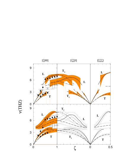
Figure 7: The solid lines are the L branch in all the three panels, the dashed lines are the T branch in the left and the right panels. In the central column, the long-dashed curves are the T₁ branches while the dot-dashed curves are the T₂ branches. The shaded regions span the FWHMs. The circles in the left panels are the experimental data expt3 . The filled ones are those with better resolution and accuracy. (Top panel)Dispersion curves for Ni₅₀Pt₅₀ calculated in the ICPA. (Bottom panel)Dispersion curves for Ni₅₀Pt₅₀ calculated in the CPA. Here, the shaded regions in the left panel span the FWHMs. In other two panels the thin dotted lines denote the FWHMs.

In Fig.7, we compare the dispersion curves and widths obtained in the ICPA from the coherenet scattering structure factors, using the force constants as given above, with those in the CPA, using the averages of the same force-constants, and with the experimental results expt3 . The top three panels are the results obtained in the ICPA for the three symmetry directions. The procedure has already been discussed in the previous section. The bottom panels are the CPA results. The circles and error bars in the left panels are the experimental frequencies and the widths(FWHMs). The filled circles are experimental results with more accuracy and greater resolution. The shaded regions in the top panels and in the leftmost panel in the bottom span the calculated FWHM’s. The FWHM’s for the middle and the right panels in the bottom are indicated by the thin dotted lines. For the $[\zeta,0,0]$ and the $[\zeta,\zeta,\zeta]$ directions, the solid lines represent the longitudinal modes and the dotted lines the transverse modes. For the $[\zeta,\zeta,0]$ direction, the solid lines show the longitudinal mode while the long-dashed and the dot-dashed curves stand for the T₁ and the T₂ transverse modes, respectively. The experimental results are available only for the $[\zeta,0,0]$ directions in this system. The ICPA agrees much better with the experiments than the CPA for both the longitudinal and the transverse branches. The CPA frequencies are generally below the experimental ones at low frequencies and above the experimental ones at high frequencies. The discrepancy gets worse as we move from the middle of the zone towards the zone edge. This can be explained the following way: the high wave-vector region is dominated by the lighter atoms. The use of the average force-constants by the CPA coupled with the domination of the lighter mass pushes the frequencies further up, thus producing a significant deviation from the experimental ones. The severity of this effect can be understood from the widths as well. In the CPA, the experimental points stay well outside the disorder-induced widths centered at the peak frequencies. The discrepancy is substantially reduced by the inclusion of force-constant disorder, as is seen from the ICPA results. Its inclusion changes the dispersion curves qualitatively as well. In the CPA, the bands extend fully across the Brilluoin zone for all symmetry directions while in the ICPA, the Pt-dominated peaks disappear at high-$\zeta$ and the Ni-dominated peaks wash out at low-$\zeta$ for all modes and symmetry directions, an effect observed in the experiments. This is a clear consequence of the force-constant disorder which can be understood by inspecting the spectral line shapes. In Fig.8(a) we present the partial and the total spectral densities for three different wave-vectors, one on the lower side of the zone, one in the middle and one at the boundary. The solid lines are the total spectral functions, the dotted lines are the Ni-Ni partial spectral functions, the long-dashed lines are the Pt-Pt contributions while the dot-dashed lines are the Ni-Pt contributions. In Fig.8(b) we present the partial and the total coherent scattering structure factors i.e. the spectral functions weighted by the coherent scattering lengths of the species. The coherent scattering lengths of Ni and Pt differ by only 7$\%$(the scattering length of Ni is 1.03 while that of Pt is 0.95), much less than do those of Ni and Pd. However, even this small difference produces significant changes in the line shapes and in the peak frequencies. In Fig.8(b), the solid lines give the total structure factor, the dotted lines are for weighted Ni-Ni contributions, the long-dashed lines give the weighted Pt-Pt contributions and the dot-dashed lines stand for weighted Ni-Pt contributions. A close inspection of the various contributions reveals the fact that unlike in NiPd, the Ni-Pt contribution plays the key role in determining the weight in the middle of the band (and in obtaining the merged bands in Fig.6) as well as adding or subtracting weights to the Ni-Ni or Pt-Pt contributions, thus elevating or suppressing one of the peaks. For example, in Fig.8(a), in the [.5,0,0]T curves, the Ni-Pt contribution adds weight to the total spectral function on top of the Pt-Pt peak at the low frequenies while it subtracts weight from the Ni-Ni contribution at higher frequencies thereby causing a weakly defined peak at high frequencies. In the [.5,0,0]L and in the [1,0,0]T curves, the Ni-Pt contribution adds weight between the Pt-Pt and Ni-Ni peaks, thereby removing the gap in the spectrum. The Ni-Pt contribution is totally due to inclusion of force-constant disorder, since diagonal disorder produces no such contribution. Thus, the CPA produces spectral functions having two well-defined peaks corresponding to the Ni-Ni and the Pt-Pt contributions with a gap in between resulting in extended dispersion curves and split bands. The effect of incorporation of the difference in scattering lengths can be seen from these two figures as well. For example, in the [1,0,0]T curves, there are two well-defined peaks in the total spectral functions, whereas the low-frequency peak is transformed into a shoulder in the total structure factor. This is because Ni has the larger scattering length which enhances the weight associated with the Ni-Pt contribution thereby cancelling more effectively the contribution from the Pt-Pt part. Similar effects are seen in the [.5,0,0]L and [1,0,0]L curves. Moreover, this weighting sometimes produces a weakly defined peak whose FWHM cannot be well determined, which explains the observed washing out of the dispersion curves noted above. The effect of the small difference in scattering lengths is amplified by the force-constant disorder through the Ni-Pt structure factor.

Figure 8: (a)Partial and total spectral functions calculated in the ICPA for various $\zeta$ values in the [$\zeta$,0,0] directions in Ni₅₀Pt₅₀. (b) Partial and total structure factors calculated in the ICPA for various $\zeta$ values in the [$\zeta$,0,0] directions in Ni₅₀Pt₅₀. The solid lines are the total contributions, the dotted lines are the Ni-Ni contributions, the long-dashed lines are the Pt-Pt contributions and the dot-dashed lines are the Ni-Pt contributions. The details are given in the text.

In sum, the force-constant disorder plays a significant role in Ni₅₀Pt₅₀, and a theory with mass disorder only, like the CPA, fails both qualitatively and quantitatively in such cases. On the other hand, the ICPA successfully explains the effects of force-constant disorder through its effect on the partial structure factors. It also demonstrates the relative importance of the contributions of various atomic species to the coherent and incoherent structure factors which the CPA cannot. The ICPA and the Ni₅₀Pt₅₀ system therefore provide a proper test case for force-constant disorder and show that the ICPA can form a basis for understanding the lattice dynamics of other binary alloys.

VI Conclusions

We have presented a straight-forward and tractable formulation of the KLGD klgd method for single-site scattering of phonons in three dimensional lattices. We have demonstrated how this multiple-scattering based formalism captures the effects of off-diagonal and environmental disorder. The use of augmented-space to keep track of the configurations of the system has made the formalism simple yet powerful. The resulting translational invariance makes it numerically tractable as well. A significant contribution beyond Ref.18 is the derivation of the partial Green’s functions in real-space and the derivation of the partial spectral functions as well as their sum rules. This enables one to make direct comparison with neutron scattering experiments because of the incorporation of the scattering lengths of the different species. We have applied the formalism to real random alloys for the first time. In Ni₅₅Pd₄₅ we have demonstrated that mass disorder plays the prominent role, and the CPA consequently does a rather good job whereas the mean-crystal model requires erroneous fitted force-constants. Our partial structure factors enable us to understand the insensitivity of the normal modes towards the difference in the coherent scattering lengths of the two species despite the significant difference of 43$\%$ in this system. The Ni₅₀Pt₅₀ results demonstrate the prominence of force-constant disorder even in a case where the mass ratio is 3. The ICPA agrees well with both the coherent and the incoherent scattering experiments, whereas the CPA fails, both quantitatively and qualitatively. We are able to establish the role of the force-constant differences between the species in great detail with the help of the partial spectral functions and the partial structure factors. We have consequently clearly demonstrated that for systems like NiPt, where the force-constants are strongly species dependent, the determination of their values is crucial. However, we had no prior information about the species dependence of the force-constants. Intuitive arguments led to a set of force-constants which turned out to be quite good. A better understanding of the role of disorder in the lattice dynamics of random alloys could be achieved with prior information about the force-constants. These could be obtained, e.g., from first principles calculations on a set of ordered alloys.

Appendix A Matrix elements

For the calculations in the nearest-neighbor approximation, one needs to evaluate the $\{3\left(Z+1\right)\}^{2}$ matrix elements of the operators ${\bf K}^{\prime}$, ${\bf K}^{\prime\dagger}$, $\widetilde{\bf V}\left(\vec{q}\right)$ and ${\bf G}_{vca}^{-1}$ and use them as inputs. These evaluations are done in augmented space using Eq.(14). The symmetry of the lattice structure is used to reduce the number of matrix elements evaluated. Here, we give results only for an fcc lattice. All the matrices are, therefore, of dimension $39\times 39$.

In an fcc system, each atom has 12 nearest neighbors with coordinates $\left(\pm\frac{1}{2},\pm\frac{1}{2},0\right)$, $\left(\pm\frac{1}{2},0,\pm\frac{1}{2}\right)$, and $\left(0,\pm\frac{1}{2},\pm\frac{1}{2}\right)$ with respect to the coordinates of the reference atom at $\left(0,0,0\right)$. The force-constants, between the atom $0$ and its neighbors satisfy the following cubic symmetry relation.

$$\phi^{\alpha\beta}_{0j}=\phi^{\beta\alpha}_{0j}=\phi^{\alpha\beta}_{j0}=\phi^{\alpha\beta}_{0k},$$ (69)

where $\vec{R}_{0j}=-\vec{R}_{0k}$ and $k$ and $j$ are two neighbors on opposite sides of site $0$. For example, the force-constant matrix between the atoms $\left(0,0,0\right)$ and $\left(\frac{1}{2},\frac{1}{2},0\right)$ is of the form,

$$\phi_{(000,\frac{1}{2}\frac{1}{2}0)}=\left(\begin{array}[]{ccc}a&b&0\\ b&a&0\\ 0&0&g\end{array}\right).$$ (70)

The force-constant matrices between the atom $0$ and its other neighbors can easily be calculated from (A2) via the cubic symmetry operations. The results are:

$$\left(G_{vca}^{-1}\right)^{\alpha\beta}_{ij} = \bar{m}\omega^{2}-8D_{1}^{xx}-4D_{1}^{\prime xx}\text{\hskip 56.9055pt}\text{if $i=j$, $\alpha=\beta$},$$ (71)

$$= 0\text{\hskip 145.10922pt}\text{if $i=j$, $\alpha\neq\beta$},$$

$$= D_{1}^{\prime xx}\text{\hskip 128.0374pt}\text{ if $i=0$, $j=n=1-12$, $\alpha=\beta$, $R^{\alpha}_{j}=0$},$$

$$= D_{1}^{xx}\text{\hskip 133.72786pt}\text{if $i=0$, $j=n=1-12$, $\alpha=\beta$, $R^{\alpha}_{j}\neq 0$ },$$

$$= 2R^{\alpha}_{j}\times 2R^{\beta}_{j}\times D_{1}^{xy}\text{\hskip 73.97733pt}\text{if $i=0$, $j=n=1-12$, $\alpha\neq\beta$},$$

$$= 0\text{\hskip 147.95424pt}\text{otherwise},$$

and

$$\left(G_{vca}^{-1}\right)^{\alpha\beta}_{ij}=\left(G_{vca}^{-1}\right)^{\alpha\beta}_{ji}=\left(G_{vca}^{-1}\right)^{\beta\alpha}_{ij},\text{\hskip 14.22636pt}\text{for all $i$,$j$,$\alpha$, and $\beta$}.$$

Also, we find

$$\left(K^{\prime}\right)^{\alpha\beta}_{ij} = m^{\prime}\omega^{2}-8D_{2}^{xx}-4D_{2}^{\prime xx}\text{\hskip 56.9055pt}\text{if $i=j=0$, $\alpha=\beta$},$$ (72)

$$= 0\text{\hskip 147.95424pt}\text{if $i=j=0$, $\alpha\neq\beta$},$$

$$= D_{2}^{\prime xx}\text{\hskip 128.0374pt}\text{ if $i=0$, $j=n=1-12$, $\alpha=\beta$, $R^{\alpha}_{j}=0$},$$

$$= D_{2}^{xx}\text{\hskip 133.72786pt}\text{if $i=0$, $j=n=1-12$, $\alpha=\beta$, $R^{\alpha}_{j}\neq 0$ },$$

$$= 2R^{\alpha}_{j}\times 2R^{\beta}_{j}\times D_{2}^{xy}\text{\hskip 73.97733pt}\text{if $i=0$, $j=n=1-12$, $\alpha\neq\beta$},$$

$$= -\left(K^{\prime}\right)^{\alpha\beta}_{0j}\text{\hskip 110.96556pt}\text{if $i\neq 0$, $j=i=n=1-12$},$$

$$= 0\text{\hskip 147.95424pt}\text{otherwise},$$

and

$$\left(K^{\prime}\right)^{\alpha\beta}_{ij}=\left(K^{\prime}\right)^{\alpha\beta}_{ji}=\left(K^{\prime}\right)^{\beta\alpha}_{ij},\text{\hskip 14.22636pt}\text{for all $i$,$j$,$\alpha$, and $\beta$}.$$

Similarly, we obtain

$$\widetilde{V}\left(\vec{q}\right)^{\alpha\beta}_{ij} = L^{\alpha}\text{\hskip 159.3356pt}\text{if $i=j=0$, $\alpha=\beta$},$$ (73)

$$= 4D_{3}^{xy}Sin(q_{\alpha})Sin(q_{\beta})\text{\hskip 79.6678pt}\text{if $i=j=0$, $\alpha\neq\beta$},$$

$$= D_{5}\text{\hskip 153.6447pt}\text{ if $i=0$, $j=n=1-12$, $\alpha=\beta$, $R^{\alpha}_{j}=0$},$$

$$= D_{6}\text{\hskip 156.49014pt}\text{if $i=0$, $j=n=1-12$, $\alpha=\beta$, $R^{\alpha}_{j}\neq 0$ },$$

$$= 2R^{\alpha}_{j}\times 2R^{\beta}_{j}\times D_{7}\text{\hskip 96.73918pt}\text{if $i=0$, $j=n=1-12$, $\alpha\neq\beta$},$$

$$= D_{4}^{\prime xx}-D_{1}^{\prime xx}\text{\hskip 113.81102pt}\text{ if $i\neq 0$, $j=i=n=1-12$, $\alpha=\beta$, $R^{\alpha}_{i}=0$},$$

$$= D_{4}^{xx}-D_{1}^{xx}\text{\hskip 122.34692pt}\text{if $i\neq 0$, $j=i=n=1-12$, $\alpha=\beta$, $R^{\alpha}_{i}\neq 0$ },$$

$$= 2R^{\alpha}_{j}\times 2R^{\beta}_{j}\times\left(D_{4}^{xy}-D_{1}^{xy}\right)\text{\hskip 51.21504pt}\text{if $i\neq 0$, $j=i=n=1-12$, $\alpha\neq\beta$},$$

$$= -D_{3}^{\prime xx}e^{i\vec{q}\cdot\vec{R}_{i}}\text{\hskip 119.50148pt}\text{if $j\neq i=n=1-12$, $\vec{R}_{j}=-\vec{R}_{i}$, $\alpha=\beta$, $R_{j}^{\alpha}=0$},$$

$$= -D_{3}^{xx}e^{i\vec{q}\cdot\vec{R}_{i}}\text{\hskip 122.34692pt}\text{if $j\neq i=n=1-12$, $\vec{R}_{j}=-\vec{R}_{i}$, $\alpha=\beta$, $R_{j}^{\alpha}\neq 0$},$$

$$= -D_{3}^{xy}e^{i\vec{q}\cdot\vec{R}_{i}}\times 2R_{i}^{\alpha}\times 2R_{i}^{\beta}\text{\hskip 62.59596pt}\text{if $j\neq i=n=1-12$, $\vec{R}_{j}=-\vec{R}_{i}$, $\alpha\neq\beta$},$$

$$= 0\text{\hskip 165.02606pt}\text{otherwise},$$

and

$$\widetilde{V}\left(\vec{q}\right)^{\alpha\beta}_{ij} = \left(\widetilde{V}\left(\vec{q}\right)^{\star}\right)^{\alpha\beta}_{ji}=\widetilde{V}\left(\vec{q}\right)^{\beta\alpha}_{ij},\text{\hskip 14.22636pt}\text{for all $i$,$j$,$\alpha$, and $\beta$}.$$

In these evaluations, we have used the notation $R_{0j}=R_{j}$, $n=1-12$ to represent the 12 nearest neighbors, and the notations

$$\bar{m} = c_{A}m^{A}+c_{B}m^{B},$$

$$m^{\prime} = \sqrt{c_{A}c_{B}}\left(m^{A}-m^{B}\right),$$

$$\tilde{m} = c_{B}m^{A}+c_{A}m^{B},$$

$$D_{1}^{xx} = c_{A}^{2}a_{AA}+c_{B}^{2}a_{BB}+2c_{A}c_{B}a_{AB},$$

$$D_{1}^{\prime xx} = c_{A}^{2}g_{AA}+c_{B}^{2}g_{BB}+2c_{A}c_{B}g_{AB},$$

$$D_{1}^{xy} = c_{A}^{2}b_{AA}+c_{B}^{2}b_{BB}+2c_{A}c_{B}b_{AB},$$

$$D_{2}^{xx} = \sqrt{c_{A}c_{B}}\{c_{A}a_{AA}-c_{B}a_{BB}+(c_{B}-c_{A})a_{AB}\},$$

$$D_{2}^{\prime xx} = \sqrt{c_{A}c_{B}}\{c_{A}g_{AA}-c_{B}g_{BB}+(c_{B}-c_{A})g_{AB}\},$$

$$D_{2}^{xy} = \sqrt{c_{A}c_{B}}\{c_{A}b_{AA}-c_{B}b_{BB}+(c_{B}-c_{A})b_{AB}\},$$

$$D_{3}^{xx} = c_{A}c_{B}\left(a_{AA}+a_{BB}-2a_{AB}\right),$$

$$D_{3}^{\prime xx} = c_{A}c_{B}\left(g_{AA}+g_{BB}-2g_{AB}\right),$$

$$D_{3}^{xy} = c_{A}c_{B}\left(b_{AA}+b_{BB}-2b_{AB}\right),$$

$$D_{4}^{xx} = c_{A}c_{B}\left(a_{AA}+a_{BB}\right)+\left(c_{A}^{2}+c_{B}^{2}\right)a_{AB},$$

$$D_{4}^{\prime xx} = c_{A}c_{B}\left(g_{AA}+g_{BB}\right)+\left(c_{A}^{2}+c_{B}^{2}\right)g_{AB},$$

$$D_{4}^{xy} = c_{A}c_{B}\left(b_{AA}+b_{BB}\right)+\left(c_{A}^{2}+c_{B}^{2}\right)b_{AB},$$

$$D_{5} = \left(D_{1}^{xx}-D_{4}^{xx}\right)+D_{3}^{xx}e^{i\vec{q}\cdot\vec{R}_{j}},$$

$$D_{6} = \left(D_{1}^{xy}-D_{4}^{xy}\right)+D_{3}^{xy}e^{i\vec{q}\cdot\vec{R}_{j}},$$

$$D_{7} = \left(D_{1}^{\prime xx}-D_{4}^{\prime xx}\right)+D_{3}^{\prime xx}e^{i\vec{q}\cdot\vec{R}_{j}},$$

$$L^{\alpha} = \left(\bar{m}-\tilde{m}\right)\omega^{2}-8\left(D_{1}^{xx}-D_{4}^{xx}\right)-4\left(D_{1}^{\prime xx}-D_{4}^{\prime xx}\right)-4D_{3}^{xx}\{Cos\enskip q_{\alpha}\left(Cos\enskip q_{\gamma}+Cos\enskip q_{\delta}\right)$$ (74)

$$\text{\hskip 113.81102pt}-4D_{3}^{\prime xx}Cos\enskip q_{\gamma}Cos\enskip q_{\delta};\text{\hskip 56.9055pt}\gamma,\delta\neq\alpha.$$

The symmetries of the force-constant matrices are reflected in the operators as well. The effect of itineration is captured in $\widetilde{V}\left(\vec{q}\right)^{\alpha\beta}_{ij}$ through the quantities $D_{3}^{\alpha\beta}$. When there is no force-constant disorder the $D_{3}$ terms vanish, and $\widetilde{\bf V}$ becomes independent of $\vec{q}$. A $\vec{q}$-independent self-energy results, and we arrive at the CPA equations. To illustrate how to obtain the various matrix elements of the operators, we present the calculation of $K^{\prime(0)}_{01}$ where $R_{1}=\left(\frac{1}{2},\frac{1}{2},0\right)$.

$$K^{\prime(0)}_{01} = \langle 0f|\widehat{\bf K}|1f_{0}\rangle,$$

$$= \langle 0f|\left(\widehat{\bf m}\omega^{2}-\widehat{\bf\Phi}\right)|1f_{0}\rangle.$$

Using Eqs.(6)and (11),

$$\langle 0f|\widehat{\bf m}|1f_{0}\rangle = 0,$$

and using Eqs.(7) and (11),

$$\langle 0f|\widehat{\bf\Phi}|1f_{0}\rangle = \langle f|\widehat{\bf\Phi}_{01}|f_{0}\rangle,$$

$$= \langle\left(\sqrt{c_{A}}\langle A_{0}|+\sqrt{c_{B}}\langle B_{0}|\right),\left(\sqrt{c_{A}}\langle A_{1}|+\sqrt{c_{B}}\langle B_{1}|\right)|\{\phi_{01}^{AA}\widehat{\bf\eta}_{0}^{A}\widehat{\bf\eta}_{1}^{A}+\phi_{01}^{BB}\widehat{\bf\eta}_{0}^{B}\widehat{\bf\eta}_{1}^{B}+\phi_{01}^{AB}\widehat{\bf\eta}_{0}^{A}\widehat{\bf\eta}_{1}^{B}+\phi_{01}^{BA}\widehat{\bf\eta}_{0}^{B}\widehat{\bf\eta}_{1}^{A}\}|$$

$$\text{\hskip 142.26378pt}\left(\sqrt{c_{B}}|A_{0}\rangle-\sqrt{c_{A}}|B_{0}\rangle\right),\left(\sqrt{c_{A}}|A_{1}\rangle+\sqrt{c_{B}}|B_{1}\rangle\right)\rangle.$$

If we use the cartesian coordinates explicitly, then the xx component is, for example,

$$\langle f|\Phi^{xx}_{01}|f_{0}\rangle = \sqrt{c_{A}c_{B}}\{c_{A}a_{AA}-c_{B}a_{BB}+(c_{B}-c_{A})a_{AB}\}$$

$$= D_{2}^{xx}.$$

The other components can be calculated similarly.

References

- (1) B. Mozer, K. Otnes and V. W. Myers, Phys. Rev. Lett. 8, 278 (1962); B. Mozer, K. Otnes and C. Thaper, Phys. Rev. 152 535 (1966); E. C. Svensson, B. N. Brockhouse and J.M. Rowe, Solid State Commun. 3, 245 (1965); E. C. Svensson and B. N. Brockhouse, Phys. Rev. Lett. 18, 858 (1967); H. G. Smith and M. K. Wilkinson, Phys. Rev. Lett. 20, 1245 (1968); R. M. Nicklow, P. R. Vijayraghavan, H. G. Smith and M. K. Wilkinson, in Neutron Inelastic Scattering (IAEA, Vienns, 1968), Vol I, p. 47.
- (2) R. M. Cunnigham, L. D. Muhlestein, W. M. Shaw and C. W. Tompson , Phys. Rev. B 2, 4864 (1970); N. Wakabayashi, R.M. Nicklow and H. G. Smith , Phys. Rev. B 4, 2558 (1971); E. C. Svensson and W. A. Kamitakahara , Can. J. Phys. 49, 2291 (1971); N. Wakabayashi, Phys. Rev. B 8, 6015 (1973); B. N. Brockhouse and R. M. Nicklow, Bull. Am. Phys. Soc. 18, 112 (1973); A. Zinken, U. Buchenau, H. J. Fenzel and H. R. Schober. Solid State Commun. 13, 495 (1977)
- (3) W. A. Kamitakahara and B. N. Brockhouse, Phys. Rev. B 10, 1200 (1974)
- (4) Y. Tsunoda, N. Kunitomi, N. Wakabayashi, R.M. Nicklow and H. G. Smith, Phys. Rev. B 19, 2876 (1979)
- (5) R. M. Nicklow in Methods of Experimental Physics (Academic Press, 1983), Vol 23, p. 172
- (6) D. W. Taylor, Phys. Rev. 156, 1017 (1967)
- (7) N. Kunimoto, Y. Tsunoda and Y. Hirai, Solid State Commun. 13, 495 (1973); T. Kaplan and M. Mostoller, Phys. Rev. B. 9, 353 (1974); W. A. Kamitakahara, Bull. Am. Phys. Soc. 19, 321 (1974)
- (8) W. A. Kamitakahara and D. W. Taylor, Phys. Rev. B. 10, 1190(1974); M. Mostoller, T. Kaplan, N. Wakabayashi and R. M. Nicklow, Phys. Rev. B. 10, 3144 (1974); H. G. Smith and N. Wakabayashi, Bull. Am. Phys. Soc. 21, 410 (1976)
- (9) H. Shiba, Prog. Theor. Phys. 40, 942 (1968)
- (10) T. Kaplan and M. Mostoller, Phys. Rev. B. 9, 1783 (1974)
- (11) S. Takeno, Prog. Theor. Phys. 40, 942 (1968)
- (12) B. G. Nickel and W. H. Butler, Phys. Rev. Lett. 30, 363 (1973)
- (13) F. Ducastelle, J. Phys. C 7, 1795 (1974); J. Mertsching, Phys. Status Solidi B, 63, 241 (1974)
- (14) A. Gonis and J. W. Garland, Phys. Rev. B. 18, 3999 (1978)
- (15) R. Haydock, V. Heine and M. J. Kelly, J. Phys. C:Solid State Phys. 5 , 2845 (1975)
- (16) M. Yussouff and A. Mookerjee, J. Phys. C: Solid State Phys. 17, 1009 (1984)
- (17) A. Mookerjee, J. Phys. C:Solid State Phys. 6, L205 (1973)
- (18) T. Kaplan, P. L. Leath, L. J. Gray and H. W. Diehl, Phys. Rev. B 21, 4230 (1980)
- (19) R. Mills and P. Ratanavararaksha, Phys. Rev. B 18, 5291 (1978)
- (20) R.J. Elliott, J.A. Krumhansl and P.L. Leath, Rev. Mod. Phys. 46, 465(1974)
- (21) T. Kaplan and L. J. Gray, Phys. Rev. B 14, 3462 (1976)
- (22) D.H. Dutton, B.N. Brockhouse and A.P. Miller, Can. J. Phys. 50, 2915 (1972)
- (23) E.C. Svensson, B.N. Brockhouse and J.M. Rowe, Phys. Rev. 155, 619 (1967)
- (24) A. Mookerjee and R.P. Singh, J. Phys. F: Met. Phys., 18, 2171 (1988)
- (25) W.A. Kamitakahara and D.W. Taylor, Phys. Rev. B 10, 1190 (1974)
- (26) A.C. Aitken, in Determinants and Matrices(Interscience Publishers) (1956)
- (27) S.M. Chitanvis and P.L. Leath, J.Phys.C:Solid State Phys., 16, 1049 (1983)
- (28) A. Gonis, in Green functions for ordered and disordered systems (North-Holland)(1992), p. 141