Equation of State of Supercooled Water
from the Sedimentation Profile

Masako Yamada,¹ H. Eugene Stanley¹ and Francesco Sciortino² ¹Center for Polymer Studies and Department of Physics, Boston University, Boston, MA 02215 USA
²Dipartimento di Fisica, INFM UdR and INFM Center for Statistical Mechanics and Complexity, Università di Roma “La Sapienza”, Piazzale Aldo Moro 2, I-00185, Roma, Italy

(yss.tex printed )

Abstract

To study the coexistence of two liquid states of water within one simulation box, we implement an equilibrium sedimentation method—which involves applying a gravitational field to the system and measuring/calculating the resulting density profile in equilibrium. We simulate a system of particles interacting via the ST2 potential, a model for water. We detect the coexistence of two liquid phases at low temperature.

pacs:

PACS number(s):

I Introduction

The physics of the liquid state has been the subject of intense research activity. Novel approaches and novel apparatus have made possible the study of liquids under extreme thermodynamic conditions and in wide windows of space and time. Interesting and unexpected new phenomena have emerged as a result of a combined effort involving experiments, theory and simulationsDebenedetti ; MarieClaire . One of these is the possibility of a liquid-liquid (LL) transition in one-component systems—in addition to the usual liquid-gas transition. Several liquids Katayama ; Ree ; Togaya and several models StellHemmer ; GF ; Reza ; Swendsen ; Jagla ; Pablo ; Saika ; Lacks have been studied in detail, and it appears that the class of materials where a LL transition can be observed is larger than the class of tetrahedral liquids that were originally considered Angell00 possible candidates for a LL transition.

Water is one of the liquids that might possess a LL transition. Indeed, the first conjecture of a LL transition was based on a numerical study of the ST2 potential Poole , a model designed to mimic the behavior of liquid water. In the case of ST2, the two coexisting phases differ in their local structure. The low density phase is formed by an open tetrahedrally-coordinated network of hydrogen bonds, while the high density phase has a more distorted network of hydrogen bonds. Recent theoretical work has shown that the interplay between local energy, entropy, and volume which may generate a LL transition can in principle be realized by spherically-symmetric potentials GF ; Jagla .

The evaluation of the $P(\rho,T)$ equation of state (EOS) is key to test for phase coexistence (gas-liquid, liquid-crystal and LL), where $P$ , $\rho$ , and $T$ denote the pressure, density, and temperature. The numerical calculation of $P(\rho,T_{0})$ requires the study of the model for a variety of state points. The coexistence between two phases, in the appropriate temperature window, appears as a region of density values where $P$ is constant. In small-size numerical simulations is sometimes hard to observe phase transitions directly in one simulation box, in part because the free energy associated with creating an interface often stabilizes metastable phasesPanagiotopoulous . In these cases $P(\rho,T)$ does not show any flat region negative .

A different approach for studying in one single numerical simulation an entire isotherm has been proposed in Ref. Barrat (and later exploited in the experimental study of colloidal systems and in the study of crystallization profiles Ref. Piazza ; Lowen ; Allain ; Chaikin ). This approach simulates a semi-infinite tube in the presence of a very strong gravitational field and measures the density profile in equilibrium. A simple inversion of the density profile allows the model EOS to be constructed. This idea has also been applied in the experimental study of the EOS of colloidal particles, by inversion of the measured sedimentation equilibrium profile.

Here we apply the sedimentation profile method to ST2 water. We find that an interface separating two liquid states appears at low temperature, corresponding to the coexistence of two metastable liquid states of water within one simulation box, providing evidence for the presence of an LL transition.

II Theory and Simulation Details

We study $N=7680$ rigid molecules of mass $M$ interacting through the ST2 water potential, a rigid, non-polarizable, 5-site potential Stillinger that is able to reproduce qualitatively the thermodynamic anomalies of liquid water. “ST2 water” is characterized, on cooling, by isobaric density maxima, increasing compressibility, increasing constant $P$ specific heat, and evidence for a LL transition in the deeply supercooled regime (which is difficult to probe experimentally due to spontaneous crystallization Poole ).

To implement the sedimentation profile method, we use a column-shaped simulation box, semi-infinite along the $z$ axis and with periodic boundary conditions along the $x$ and $y$ axes. The top of the box is left open, while the bottom is assumed to be a repulsive soft-sphere surface, generating a short-range force proportional to $z^{-13}$ acting on the molecule center of mass (Fig. 1). The box width in the $x$ -axis and $y$ -axis directions is 3 nm, corresponding to a bottom surface area of $S_{xy}=9$ nm². A strong gravitational field $g_{s}=2\times 10^{12}g$ is applied downward, in the $z$ -axis direction, where $g=9.8$ kg/m² is the Earth’s gravitational field. The value of the field controls the range of $P$ -values accessed in the simulations. The pressure at the bottom of the column is $P=g_{s}NM/S_{xy}\simeq 500$ MPa.

We perform the simulations using a multi-processor code on SGI Origin 2000, IBM SP, and IBM Regatta supercomputers. We choose a 1 fs time step and study different temperatures from $T=300$ K down to $T=230$ K. For T= $230$ K, we simulate four different systems to better estimate error and reproducibility of the results. A long ( $\sim 10ns$ ) equilibration time precedes the actual calculation of the equilibrium density profile. To analyze equilibration we monitored the running average of the $z$ -position of the center of mass. Production runs lasted at least 200 ps for the higher temperatures up to several ns per box when $T=230$ K.

Refer to caption — Figure 1: Schematic of the columnar box in a gravitational field $g_{s}$ . We partition the box into equally sized bins with height $\Delta z$ , where each bin represents a state point. The number of molecules in each bin is used to calculate the density and pressure at the center of the bin.

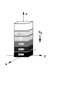
We define a mass density field $\rho(z)$ by averaging the density over bins with height $\Delta z=1$ nm to calculate the pressure field $P(z)$ from

P(z)=g\int_{z}^{\infty}\rho(z^{\prime})dz^{\prime}.

(1)

A parametric plot of $P(z)$ vs. $\rho(z)$ provides the EOS.

III Results and Discussion

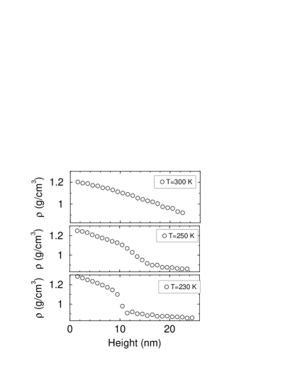
Figure 2 shows the equilibrium density profile along the $z$ -axis for three different temperatures. Each symbol represents one bin, where the height of each bin $\Delta z=1$ nm. For $T=300$ K we see only one break in the density profile: the topmost points in the plots correspond to the gas-liquid interface. Above these points is a much less dense gas not shown on this density scale. For $T=250$ K, there appears an inflection. For $T=230$ K, we see a clear break in the density, associated with the interface between two different liquid states.

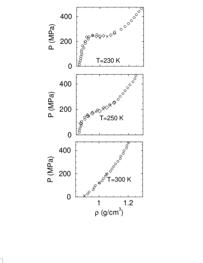
Figure 3 shows the corresponding $P(\rho)$ relations at the same three temperatures. We also show $P(\rho)$ as evaluated previously using standard MD for cubic boxes with periodic boundary conditions for systems with $N=6^{3}=216$ (Ref. peter ) and $N=12^{3}=1768$ (Ref.steve ). In Refs peter and steve $P$ was calculated with the standard virial relationnegative2 .

Consistent with the data shown in Fig. 2, we see a region of coexistence between two different phases at $T=230K$ , in agreement with the estimated location of the LL transition in Ref. Sciortino . Note that when using the sedimentation equilibration method, we see no unphysical loops in the equation of state, unlike cubic box simulations where the boundary conditions may artificially stabilize metastable states.

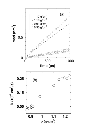
To confirm that the two coexisting phases are both liquids, we calculate the mean square displacement (MSD) for different height values, both below and above the interface. We follow the evolution of each molecule for an average mean squared displacement smaller that $\Delta z$ , so that each height value can be unambiguously assigned to an average density value. Figure 4 shows that both phases are sufficiently diffusive. The low density phase has smaller diffusivity, in agreement with previous simulations of the density dependence of the dynamics Geiger .

IV Conclusions

We studied the EOS of “ST2 water” with the sedimentation profile method, and presented evidence that the EOS at $T=230K$ shows a clear phase coexistence, between two phases which are both liquids. The observed LL coexistence in the ST2 potential phase diagram is consistent with estimate of the “critical point” being located around $T=235$ K, $P=250$ MPa, and $\rho=1.05$ g/cm³. Note that for most simple water models, the temperature and pressure scales are shifted relative to real values, thus they must be shifted to place them within an experimental contextcompare . The critical point estimated experimentally is around $T_{c}=230$ K and $P_{c}=50$ MPa with $\rho=1.05$ g/cm³Mishima .

Acknowledgments

This work is supported by NSF grant CHE-0096892. MY is also supported by NSF grant GER-9452651. FS thanks INFM-Iniziative Parallel Computing for granting numerical resources.

References

(1) P. G. Debenedetti, Metastable Liquids (Princeton University Press, Princeton, 1996).
(2) M.-C. Bellissent-Funel, Ed. Hydration Processes in Biology: Theoretical and Experimental Approaches [Proc. NATO Advanced Study Institutes, vol. 305) (IOS Press, Amsterdam, 1999)
(3) Y. Katayama, T. Mizutani, W. Utsumi, O. Shimomura, M. Yamakata, and K. Funakoshi, Nature 403, 170 (2000). 305) (IOS Press, Amsterdam, 1999),
(4) M. van Thiel and F. H. Ree, Phys. Rev. B. 48, 3591 (1993).
(5) M. Togaya, Phys. Rev. Lett. 79, 2474 (1997).
(6) D. J. Lacks, Phys. Rev. Lett. 84, 4629 (2000).
(7) P. C. Hemmer and G. Stell, Phys. Rev. Lett. 24, 1284 (1970).
(8) G. Franzese et al., Nature 409, 692 (2001).
(9) M. R. Sadr-Lahijany et al., Phys. Rev. Lett. 81, 4895 (1998).
(10) H. K. Lee and R. H. Swendsen, Phys. Rev. B 64, 214102 (2001).
(11) E. A. Jagla, J. Chem. Phys. 111, 8980 (1999).
(12) C. J. Roberts, A. Z. Panagiotopoulous, and P. G. Debenedetti, Phys. Rev. Letter 77, 4386 (1996).
(13) I. Saika-Vovoid et al., Phys. Rev. E 63 011202 (2001).
(14) C. A. Angell, R. D. Bressel, M. Hemmati, E. J. Sare, J. C. Tucker, Phys. Chem. Chem. Phys. 2, 1559 (2000).
(15) P. H. Poole et al., Nature 360, 324 (1992).
(16) A. Panagiotopoulous, Mol. Phys. 61, 813 (1987). The Gibbs ensemble method has been developed to allow the study of the coexisting phases in the absence of interfaces using two or more simulation boxes coupled to each other.
(17) In small-size simulation boxes, a negative slope “loop” may be seen, and the Maxwell construction method is used to calculate the critical pressure and density..
(18) T. Biben, J. P. Hansen, and J. L. Barrat, J. Chem. Phys. 98, 7330 (1993).
(19) R. Piazza, T. Bellini and V. Degiorgio, Phys. Rev. Lett. 71, 4267 (1993).
(20) L. Bocquet and H. Lowen, Phys. Rev. E. 49, 1883 (1994).
(21) C. Allain, M. Cloitre, and M. Wafra, Phys. Rev. Lett. 74, 1478 (1995).
(22) M. A. Rutgers, J. H. Dunsmuir, J.-Z. Xue, W. B. Russel, and P. M. Chaikin, Phys. Rev. B. 53, 5043 (1996).
(23) F. H. Stillinger and A. Rahman, J. Chem. Phys. 60, 1545 (1974).
(24) P. H. Poole et al., Phys. Rev. E 48, 3799 (1993).
(25) S. Harrington et al., Phys. Rev. Lett. 78, 2409 (1997).
(26) Regions of negative $P$ cannot be studied with the sedimentation method, at least not in its present form.
(27) F. Sciortino, A. Geiger, and H. E. Stanley, J. Chem. Phys. 96, 3857 (1992). We recall that in water, at low enough temperatures, there is pressure window within which particles diffuse faster with increasing pressure due to the breakage of the hydrogen-bonded network.
(28) F. Sciortino, P. H. Poole, U. Essmann, and H. E. Stanley, Phys. Rev. E 55, 727 (1997).
(29) A. Scala et al., Phys. Rev. E 62, 8016 (2000).
(30) M. Yamada, S. Mossa, H. E. Stanley, and F. Sciortino, Phys. Rev. Lett. 88, 195701 (2002).
(31) O. Mishima and H. E. Stanley, Nature 392, 164 (1998); O. Mishima, Phys. Rev. Lett. 85, 334 (2000).
(32) In comparison, the critical point estimated using the using the SPC/E potential is estimated to be $T=130$ K and $P=290$ MPa with $\rho=1.10$ g/cm³ Scala ; using the TIP4P potential $T<200$ K and $P_{c}>70$ MPa Sciortino ; and using the TIP5P potential $T_{c}\approx 217$ K, $\rho_{c}\approx 1.13$ g/cm³, and $P\approx 340$ MPa TTT .

Equation of State of Supercooled Water from the Sedimentation Profile