Band-center anomaly of the conductance distribution in one-dimensional Anderson localization

Abstract

We analyze the conductance distribution function in the one-dimensional Anderson model of localization, for arbitrary energy. For energy at the band center the distribution function deviates from the universal form assumed in single-parameter scaling theory. A direct link to the break-down of the random-phase approximation is established. Our findings are confirmed by a parameter-free comparison to the results of numerical simulations.

The spatial localization of waves in a disordered potential can be considered as the most dramatic effect of multiple coherent wave scattering sheng ; berk . Due to systematic constructive interference in some part of the medium the wave function is spatially confined and decays exponentially as one moves away from the localization center Anderson ; reviews . The localization length $l_{\rm loc}$ can be probed non-invasively from the decay of the transmission coefficient (the dimensionless conductance Landauer ) $g$, in terms of the average

$$C_{1}\equiv\langle-\ln g\rangle=2L/l_{\rm loc}+O(L^{0})$$ (1)

for system length $L\gtrsim l_{\rm loc}$ Borland . Localization results in insulating behavior of disordered solids at low temperatures Anderson ; reviews , and also can be realized in electromagnetic waveguides Genack , where it is considered as an efficient feedback mechanism for lasing in disordered active media Cao .

One of the cornerstones of the theoretical understanding of localization is the universal approach of single-parameter scaling (SPS) abrahams ; anderson1980 ; shapiro . In this theory it is assumed that the complete distribution function $P(g)$ of the conductance can be parameterized by the single free parameter $C_{1}$. The dependence of $C_{1}$ [and hence of $P(g)$] on $L$ is then found from solving a scaling equation $dC_{1}/d(\ln L)=\beta(C_{1})$, where the universal scaling function $\beta$ does not depend on $L$, nor on any microscopic parameter (like the Fermi wavelength $\lambda_{\rm F}$, the transport mean free path $l_{\rm tr}$, or the lattice constant $a$).

The distribution function $P(g)$ is completely determined by the cumulants

$$C_{n}\equiv\langle\langle(-\ln g)^{n}\rangle\rangle,$$ (2)

which are obtained as the expansion coefficients of the generating function

$$\eta(\xi)=\ln\langle g^{-\xi}\rangle=\sum_{n=1}^{\infty}C_{n}\frac{\xi^{n}}{n!}.$$ (3)

The first three cumulants are given by Eq. (1) for $C_{1}$, $C_{2}=\operatorname{var}\ln g$, and $C_{3}=\langle(\langle\ln g\rangle-\ln g)^{3}\rangle$. The SPS hypothesis can then be phrased like this: All cumulants are universal functions of $C_{1}$. In the localized regime ($C_{1}\gg 1$), the universal SPS relations take the simple form anderson1980

$$C_{n}/C_{1}=\delta_{1n}+2\delta_{2n}+O(L^{-1}).$$ (4)

These conditions are much more restrictive than the general upper bound $C_{n}=O(L/l_{\rm loc})$ from the theory of large-deviation statistics ott ; ellis : SPS assumes a lognormal distribution of $g$, with the variance of $\ln g$ determined by the mean via the universal relation $\operatorname{var}\ln g=-2\langle\ln g\rangle$. It is the violation of this relation which frequently is used to indicated the break-down of SPS theory (see, e.g., Ref. Altshuler1 ; Altshuler2 ).

In this paper we investigate $P(g)$ in the most-studied and best-understood paradigm of localization, the one-dimensional Anderson model defined by the Schrödinger equation

$$\psi_{l-1}+\psi_{l+1}=(V_{l}-E)\psi_{l}$$ (5)

on a linear chain of $L$ sites (lattice constant $a=1$) and a random potential with $\langle V_{l}\rangle=0$ and $\langle V_{l}V_{m}\rangle=2D\delta_{lm}$. The strength $D$ of the potential fluctuations is taken to be small. We analytically calculate the cumulants $C_{n}$ in the localized regime, with main focus on the energy region $|E|\ll 1$ around the band center of the disorder-free system. For $E=0$ we find the values

$$C_{2}/C_{1}=2.094,\quad C_{3}/C_{1}=0.568.$$ (6)

The ratios $C_{n}/C_{1}$ with the higher cumulants also are finite. Hence $P(g)$ complies with the restrictions of large-deviation statistics, but deviates from the special lognormal form assumed in SPS theory (this form is restored for $|E|\gtrsim D$).

The conditions for validity of SPS have been a constant subject of intense debate shapiro ; Altshuler1 ; Altshuler2 . Originally, SPS was derived within the random-phase approximation (RPA) for the scattering phase between consecutive scattering events abrahams ; anderson1980 . In the Anderson model the RPA is known to fail around the energies $E=\pm 2$ (the band edges of the disorder-free system) lifshitz , where $\lambda_{\rm F}\gtrsim l_{\rm tr}$. Indeed, the SPS relations (4) are violated for all cumulants when one comes close to the band edge ($2-|E|\lesssim D^{2/3}$) finitetimelyap , in coincidence with the expectations lifshitz ; Altshuler1 ; Altshuler2 ; Deych .

The RPA is also known to break down for the band-center case $E=0$ Stone . However, the only consequence observed so far has been a weak anomaly in the energy-dependence of $l_{\rm loc}$ (hence, also of $C_{1}$) kappus ; goldhirsch , which differs at $E=0$ by about $9\%$ from the predictions of perturbation theory Thouless1979 . Surprisingly, the violation (6) of the SPS relations (4) has not been noticed—quite the contrary, the relevance of the RPA for SPS recently has been contested Altshuler1 ; Altshuler2 within an investigation of the Lloyd model, given by Eq. (5) with a Cauchy distribution for the potential lloyd ; lifshitz . However, results obtained for the Lloyd model are not conclusive for the Anderson model and SPS, because in the Lloyd model formally $D=\infty$ and one encounters the modified universal relations $C_{2}/C_{1}=4\neq 2$, while $l_{\rm loc}$ varies smoothly with energy even around $E=0$ lifshitz . Moreover, the higher cumulants have not been investigated. In previous numerical studies, the violations may have passed unnoticed because the small deviation of $C_{2}/C_{1}$ from the SPS value probably was not considered to be significant, and again the higher cumulants have not been investigated. In this paper, we also will establish a direct link between SPS and RPA.

We now present the analytical calculation of the cumulants $C_{n}$ of $-\ln g$ in the vicinity of the band-center energy $E=0$ of the Anderson model, Eq. (5). As pointed out many years ago by Borland Borland , the dimensionless conductance $g$ in the localized regime is statistically equivalent to $\psi_{L}^{-2}$, where $\psi_{L}$ is the solution of the Schrödinger equation (5) with generic initial conditions $\psi_{0}$, $\psi_{1}=O(1)$. Because $\lambda_{\rm F}\simeq 4a$, it is useful to introduce two slowly varying fields $\phi(l)=\psi_{l}(-1)^{l/2}$ when $l$ is even, $\chi(l)=\psi_{l}(-1)^{(l+1)/2}$ when $l$ is odd, which can be considered as continuous functions with Langevin equations

$$\frac{d\phi}{dL}=\frac{1}{2}(U-E)\chi,\qquad\frac{d\chi}{dL}=\frac{1}{2}(W+E)\phi.$$ (7)

Here $U$ and $W$ independently fluctuate with $\langle U\rangle=0$, $\langle U(L_{1})U(L_{2})\rangle=4D\delta(L_{1}-L_{2})$, and analogously for $W$.

In order to calculate the wave-function decay and its fluctuations it is convenient to switch to the variables

$$u=\ln(\phi^{2}+\chi^{2}),\qquad\sin\alpha=\left(\frac{\phi}{2\chi}+\frac{\chi}{2\phi}\right)^{-1},$$ (8)

which are symmetric in $\phi$ and $\chi$. In the localized regime, $u=-\ln g$ characterizes the global decay of the wave function, while the variable $\alpha$ (parameterizing the local fluctuations) is identical to the scattering phase of the reflection amplitude $r=(\psi_{L-1}+i\psi_{L})/(\psi_{L-1}-i\psi_{L})$. This parameterization allows us to draw a direct relation between SPS and RPA: SPS will turn out to be valid when $\alpha$ is uniformly distributed over $(0,2\pi)$.

The Langevin equations (7) now can be translated into a Fokker-Planck equation for the joint distribution function $P(u,\alpha;x)$. For the sake of a compact presentation we use short-hand notations for the functions $s_{\alpha}=\sin\alpha$, $c_{\alpha}=\cos\alpha$, and introduce the rescaled position $x=DL$, as well as the rescaled energy $\varepsilon=E/D$. The Fokker-Planck equation then takes the form

$$\partial_{x}P(u,\alpha;x)=$$

$$[{\cal L}_{\alpha}^{2}+\partial_{u}\left(s_{\alpha}^{2}\partial_{u}-c_{\alpha}^{2}+2\partial_{\alpha}s_{\alpha}c_{\alpha}\right)-\varepsilon\partial_{\alpha}]P(u,\alpha;x),\qquad$$ (9)

with the linear differential operator ${\cal L}_{\alpha}=\partial_{\alpha}(1+c_{\alpha}^{2})^{1/2}$.

The behavior of $P(u,\alpha;x)$ for large $x$ can be analyzed by introducing into Eq. (9) the ansatz

$$P(u,\alpha;x)=\int_{-i\infty}^{+i\infty}\frac{d\xi}{2\pi i}\sum_{k=0}^{\infty}\exp(\mu_{k}(\xi)x-\xi u)f_{k}(\xi,\alpha),$$ (10)

where we require periodicity of $f_{k}(\xi,\alpha)$ in $\alpha$. It then follows that the functions $f_{k}(\xi,\alpha)$ solve the eigenvalue equation

$$\mu_{k}f_{k}=\left[{\cal L}_{\alpha}^{2}-\varepsilon\partial_{\alpha}+\xi(c_{\alpha}^{2}-2\partial_{\alpha}s_{\alpha}c_{\alpha})+\xi^{2}s_{\alpha}^{2}\right]f_{k},$$ (11)

in which $\xi$ appears as a parameter and $\mu_{k}(\xi)$ is the $k$th eigenvalue (arranged in descending order). In the vicinity of $\xi=0$, there is a finite gap between the largest eigenvalue $\mu_{0}$ [which vanishes for $\xi=0$, because of the normalization of $P(u,\alpha;x)$] and $\mu_{1}$. According to Eq. (10), the asymptotic behavior of the distribution function $P(u,\alpha;x)$ for large $x$ hence is governed by $\mu_{0}$, up to exponentially small corrections. A formal calculation of the moments of $u$ (i.e., of $-\ln g$) shows that the cumulant-generating function (3) is directly given by $\eta(\xi)=x\mu_{0}(\xi)$. Hence,

$$C_{n}=\mu^{(n)}n!DL,$$ (12)

where we expanded $\mu_{0}(\xi)=\sum_{n=1}^{\infty}\mu^{(n)}\xi^{n}$ into a power series.

The expansion coefficients $\mu^{(n)}$ can be calculated recursively for increasing order $n$ by solving the hierarchy of equations

$$\sum_{k=0}^{n}\mu^{(n-k)}f^{(k)} = s_{\alpha}^{2}f^{(n-2)}+(c_{\alpha}^{2}-2\partial_{\alpha}s_{\alpha}c_{\alpha})f^{(n-1)}$$ (13)

$${}+{\cal L}_{\alpha}^{2}f^{(n)}-\varepsilon\partial_{\alpha}f^{(n)},$$

which results when one introduces into Eq. (11) the power expansions for $\mu_{0}$ and for $f_{0}(\xi,\alpha)=\sum_{n=0}^{\infty}f^{(n)}(\alpha)\xi^{n}$: In each order $n$, we first integrate over $\alpha$ from $0$ to $2\pi$, which eliminates $f^{(n)}$ and hence gives $\mu^{(n)}$ in terms of the quantities $f^{(m)}$ and $\mu^{(m)}$ with $m<n$. Afterwards $f^{(n)}$ can be obtained from Eq. (13) by two integrations. The iteration is initiated for $n=0$ with $\mu^{(0)}=0$. This completely solves the problem to calculate the cumulants $C_{n}$ in the localized regime.

Let us illustrate the procedure for $E=0$. To start the iteration we consider Eq. (13) with $n=0$, given by ${\cal L}_{\alpha}^{2}f^{(0)}=0$. This differential equation is solved by the normalized function

$$f^{(0)}(\alpha)=\frac{\sqrt{2\pi}}{\Gamma^{2}(1/4)\sqrt{1+\cos^{2}\alpha}},$$ (14)

which is identical to the stationary limiting-distribution function $\lim_{x\to\infty}\int_{-\infty}^{\infty}du\,P(\alpha,u;x)$ of the variable $\alpha$.

Now the next iteration. Equation (13) with $n=1$ is given by

$${\cal L}_{\alpha}^{2}f^{(1)}(\alpha)=\left(\mu^{(1)}-c_{\alpha}^{2}+2\partial_{\alpha}s_{\alpha}c_{\alpha}\right)f^{(0)}(\alpha).$$ (15)

We first determine

$$\mu^{(1)}=\int_{0}^{2\pi}d\alpha\,c_{\alpha}^{2}f^{(0)}(\alpha)=4\frac{\Gamma^{2}(3/4)}{\Gamma^{2}(1/4)}.$$ (16)

The prediction for the inverse localization length

$$l_{\rm loc}=\Gamma^{2}(1/4)/[2D\Gamma^{2}(3/4)],$$ (17)

obtained by combining Eq. (16) with Eqs. (1) and (12), is identical to the result found in Refs. kappus ; goldhirsch . Then we solve for

$$f^{(1)}(\alpha)=(1+c_{\alpha}^{2})^{-1/2}\int_{0}^{\alpha}d\beta\,(1+c_{\beta}^{2})^{-1/2}\Big{[}$$

$$\quad{}2s_{\beta}c_{\beta}f^{(0)}(\beta)+\int_{0}^{\beta}d\gamma\,(\mu^{(1)}-c_{\gamma}^{2})f^{(0)}(\gamma)\Big{]}.\quad$$ (18)

From the next iteration $n=2$ we obtain

$$\mu^{(2)}=\int_{0}^{2\pi}d\alpha\,[(c_{\alpha}^{2}-\mu^{(1)})f^{(1)}(\alpha)+s_{\alpha}^{2}f^{(0)}(\alpha)]$$ (19)

and also $f^{(2)}(\alpha)$. Analogously we obtain $\mu^{(3)}$. With Eq. (12), this is sufficient to determine the values for the first three cumulants

$$C_{1}=0.4569\,DL,\quad C_{2}=0.9570\,DL,\quad C_{3}=0.2595\,DL.$$ (20)

They correspond to the anomalous ratios given in Eq. (6).

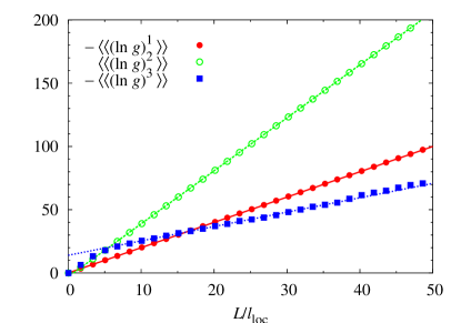
Figure 1: First three cumulants $C_{n}=\langle\langle(-\ln g)^{n}\rangle\rangle$ for energy $E=0$ in the Anderson model (5) with $D=1/150$, as function of system length $L$. The data points are the result of a numerical simulation. The slopes of the straight lines follow the predictions of Eq. (20). The localization length $l_{\rm loc}$ is taken from Eq. (17).

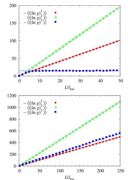
Figure 2: Same as Fig. 1, but for energy $E=0.1$ (upper panel) and $E=2$ (lower panel). The straight lines in the upper panel follow the predictions of perturbation theory Thouless1979 and single-parameter scaling anderson1980 . The straight lines in the lower panel are the predictions of Ref. finitetimelyap (see text).

The analysis of Eq. (13) can be straightforwardly carried out also for finite $E/D$. For $E/D\gg 1$, the stationary limiting-distribution function of $\alpha$ is given by $f^{(0)}(\alpha)=1/(2\pi)$, corresponding to a completely random phase. For $n=1$ we find the coefficient $\mu^{(1)}=1/2$, and the perturbative result $l_{\rm loc}=4/D$ is recovered Thouless1979 . In the next iteration we obtain $\mu^{(2)}=1/2$, while the higher coefficients all vanish. According to Eq. (12), the SPS relations (4) then are reestablished.

We have tested the predictions of the analytical theory against the result of a direct numerical computation of the conductance $g$ for the Anderson model (5), by recursively increasing the length of the wire jalabert . The potential $V_{l}$ was drawn independently for each site from a box distribution with uniform probability $1/\sqrt{24D}$ over the interval $[-\sqrt{6D},\sqrt{6D}]$. The data shown in the plots was obtained for $D=1/150$ (identical results are obtained for a Gaussian distribution with the same variance $D$). The cumulants were determined by averaging over $10^{7}$ disorder realizations.

The result of this computation for the first three cumulants and $E=0$ is shown in Fig. 1. The cumulants all increase linearly with the length $L$ of the wire, and the slopes agree perfectly with Eq. (20) [hence the localization length agrees with Eq. (17) and the ratios of cumulants agree with Eq. (6)]. The comparison is free of any adjustable parameter.

For contrast, the upper panel of Fig. 2 shows the first three cumulants at energy $E=0.1$, where the SPS relations (4) hold and $C_{1}=DL/2$ follows from perturbation theory Thouless1979 . The lower panel shows the results at the band edge $E=2$, which are compared to the predictions $C_{1}=0.7295\,D^{1/3}L$, $C_{2}=1.602\,D^{1/3}L$, $C_{3}=0.7801\,D^{1/3}L$ of Ref. finitetimelyap .

In Fig. 3 we show the ratios of cumulants $C_{2}/C_{1}$ and $C_{3}/C_{1}$ as a function of energy. The inset shows $C_{1}$. The anomalous region extends up to $E\simeq 10D$. Around the band edge, the violations set in for $2-E\lesssim 3D^{2/3}$. Again, perfect agreement is found between our analytical theory and the results of the numerical simulations.

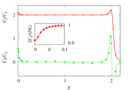
Figure 3: Energy dependence of the ratios of cumulants $C_{2}/C_{1}$ and $C_{3}/C_{1}$. The inset shows $C_{1}$ in units of the perturbative result $DL/2$. The data points are the result of a numerical simulation of the Anderson model with $D=1/150$. The curves are the analytical predictions of this paper ($E<0.1$), of perturbation theory Thouless1979 and single-parameter scaling anderson1980 ($0.1<E<1.8$), and of Ref. finitetimelyap ($E>1.8$).

In summary, we have presented an analytical theory for the distribution function $P$ of the dimensionless conductance $g$ in the localized regime of the Anderson model, Eq. (5). The relations (4) implied by single-parameter scaling theory for the cumulants $C_{n}$ of $-\ln g$ are violated not only around the band edges $|E|=2$, but also at the band-center energy $E=0$, where the correct values are given by Eq. (6). Since the random-phase approximation is known to break down in both cases, our findings reestablish the relevance of this approximation for single-parameter scaling, which recently has been contested Altshuler1 ; Altshuler2 .

Whether the single-parameter scaling hypothesis itself breaks down at $E=0$, or just persists in modified form, is an open question. The ratios (6) still imply universal relations between the cumulants for weak on-site disorder, i.e., they do not depend on the distribution function of the random potential. However, it can be questioned whether this universality also extends to additional disorder in the hopping rates, since it is well known that the extreme case of purely off-diagonal disorder results in delocalization at $E=0$ Dyson .

References

- (1) P. Sheng, Scattering and Localization of Classical Waves in Random Media (World Scientific, Singapore, 1990).
- (2) R. Berkovits and S. Feng, Phys. Rep. 238, 135 (1994).
- (3) P. W. Anderson, Phys. Rev. 109, 1492 (1958).
- (4) For reviews on localization see, e.g., P. A. Lee and T. V. Ramakrishnan, Rev. Mod. Phys. 57, 287 (1985); B. Kramer and A. MacKinnon, Rep. Prog. Phys. 56, 1469 (1993); C. W. J. Beenakker, Rev. Mod. Phys. 69, 731 (1997); A. D. Mirlin, Phys. Rep. 326, 259 (2000).
- (5) R. Landauer, Philos. Mag. 21, 863 (1970).
- (6) R. E. Borland, Proc. R. Soc. London A 274, 529 (1963).
- (7) N. Garcia and A. Z. Genack, Phys. Rev. Lett. 66, 1850 (1991); A. Z. Genack and N. Garcia, Phys. Rev. Lett. 66, 2064 (1991); D. S. Wiersma, P. Bartolini, A. Lagendijk, and R. Righini, Nature 390, 671 (1997).
- (8) A. L. Burin, M. A. Ratner, H. Cao, and S. H. Chang, Phys. Rev. Lett. 88, 093904 (2002).
- (9) E. Abrahams, P. W. Anderson, D. C. Licciardello, and T. V. Ramakrishnan, Phys. Rev. Lett. 42, 673 (1979).
- (10) P. W. Anderson, D. J. Thouless, E. Abrahams, and D. S. Fisher, Phys. Rev. B 22, 3519 (1980).
- (11) B. Shapiro, Phil. Mag. B 56, 1031 (1987); A. Cohen, Y. Roth, and B. Shapiro, Phys. Rev. B 38, 12125 (1988).
- (12) R. S. Ellis, Entropy, Large Deviations and Statistical Mechanics (Springer, New York, 1985).
- (13) E. Ott, Chaos in Dynamical Systems (Cambridge University Press, Cambridge, 1993).
- (14) L. I. Deych, A. A. Lisyansky, and B. L. Altshuler, Phys. Rev. Lett. 84, 2678 (2000).
- (15) L. I. Deych, A. A. Lisyansky, and B. L. Altshuler, Phys. Rev. B 64, 224202 (2001).
- (16) I. M. Lifshitz, S. A. Gredeskul, and L. A. Pastur, Introduction to the Theory of Disordered Systems (Wiley, New York, 1988).
- (17) H. Schomerus and M. Titov, preprint cond-mat/0204371 (2002).
- (18) L. I. Deych, M. V. Erementchouk, and A. A. Lisyansky, cond-mat/0207169 (2002).
- (19) A. D. Stone, D. C. Allan, and J. D. Joannopoulos, Phys. Rev. B 27, 836 (1983).
- (20) M. Kappus and F. Wegner, Z. Phys. B 45, 15 (1981).
- (21) I. Goldhirsch, S. H. Noskowicz, and Z. Schuss, Phys. Rev. B 49, 14504 (1994).
- (22) D. J. Thouless, in Ill-Condensed Matter, edited by R. Balian, R. Maynard, and G. Toulouse (North-Holland, Amsterdam, 1979).
- (23) P. Lloyd, J. Phys. C 2, 1717 (1969).
- (24) H. U. Baranger, D. P. DiVincenzo, R. A. Jalabert, and A. D. Stone, Phys. Rev. B 44, 10637 (1991).
- (25) G. Theodorou and M. H. Cohen, Phys. Rev. B 13, 4597 (1976); T. P. Eggarter and R. Riedinger, Phys. Rev. B 18, 569 (1978).