The Hamiltonian Mean Field Model: from Dynamics to Statistical Mechanics and back

Abstract

The thermodynamics and the dynamics of particle systems with infinite-range coupling display several unusual and new features with respect to systems with short-range interactions. The Hamiltonian Mean Field (HMF) model represents a paradigmatic example of this class of systems. The present study addresses both attractive and repulsive interactions, with a particular emphasis on the description of clustering phenomena from a thermodynamical as well as from a dynamical point of view. The observed clustering transition can be first or second order, in the usual thermodynamical sense. In the former case, ensemble inequivalence naturally arises close to the transition, i.e. canonical and microcanonical ensembles give different results. In particular, in the microcanonical ensemble negative specific heat regimes and temperature jumps are observed. Moreover, having access to dynamics one can study non-equilibrium processes. Among them, the most striking is the emergence of coherent structures in the repulsive model, whose formation and dynamics can be studied either by using the tools of statistical mechanics or as a manifestation of the solutions of an associated Vlasov equation. The chaotic character of the HMF model has been also analyzed in terms of its Lyapunov spectrum.

1 Introduction

Long-range interactions appear in the domains of gravity paddyhmf ; chavanishmf and of plasma physics elskenshmf and make the statistical treatment extremely complex. Additional features are present in such systems at short distances: the gravitational potential is singular at the origin and screening phenomena mask the Coulomb singularity in a plasma. This justifies the introduction of simplified toy models that retain only the long-range properties of the force, allowing a detailed description of the statistical and dynamical behaviors associated to this feature. In this context a special role is played by mean-field models, i.e. models where all particles interact with the same strength. This constitutes a dramatic reduction of complexity, since in such models the spatial coordinates have no role, since each particle is equivalent. However, there are several preliminary indications that behaviors found in mean-field models extend to cases where the two-body potential decays at large distances with a power smaller than space dimension tamahmf ; BMRhmf ; campa .

The Blume-Emery-Griffiths (BEG) mean-field model is discussed in this book BMRhmf and represents an excellent benchmark to discuss relations between canonical and microcanonical ensembles. Indeed, this model is exactly solvable in both ensembles and is, at the same time, sufficiently rich to display such interesting features as negative specific heat and temperature jumps in the microcanonical ensemble. Since these effects cannot be present in the canonical ensemble, this rigorously proves ensemble inequivalence. However, the BEG model has no dynamics and only the thermodynamical behavior can be investigated. Moreover, it is a spin model where variables take discrete values. It would therefore be amenable to introduce a model that displays all these interesting thermodynamical effects, but for which one would also dispose of an Hamiltonian dynamics with continuous variables, whose equilibrium states could be studied both in the canonical and in the microcanonical ensemble. Having access to dynamics, one could moreover study non equilibrium features and aspects of the microscopic behavior like sensitivity to initial conditions, expressed by the Lyapunov spectrum Ruelleeckman . Such a model has been introduced in Ref. Antoni and has been called the Hamiltonian Mean Field (HMF) model. In the simpler version, it represents a system of particles moving on a circle, all coupled by an equal strength attractive or repulsive cosine interaction. An extension of it to the case in which particles move on a 2D torus has been introduced in Ref. at and it has been quite recently realized that all such models are particular cases of a more general Hamiltonian art .

The HMF model, that we introduce in Section 2, is exactly solvable in the canonical ensemble by a Hubbard-Stratonovich transformation. The solution in the microcanonical ensemble can be obtained only under certain hypotheses that we will discuss in Section 3, but detailed information on the behavior in the microcanonical ensemble can be obtained by direct molecular dynamics (MD) simulations. The model has first and second order phase transitions and tricritical points. Its rich phase diagram allows to test the presence of ensemble inequivalence near canonical first order phase transitions and, indeed, we find negative specific heat and temperature jumps in the microcanonical ensemble. Having access to dynamics, one can study metastability of out-of-equilibrium states. This is done in Section 4, where we analyze the emergence of a coherent structure in the repulsive HMF at low energy. Similar features are also discussed in another chapter of this book tsallisrap for the attractive case near the second order phase transition. Section 5 is devoted to the study of the spectrum of Lyapunov exponents. The maximal exponent has a peak near the phase transition at ; lat1hmf ; celiahmf and vanishes when increasing the number of particles with a universal scaling law in the whole high energy disordered phase. In a low energy range the Lyapunov spectrum has a thermodynamic limit distribution similar to the one observed for systems with short-range interaction livipolruffo .

2 The HMF models

A generic two-body potential in a two dimensional square box of side $2\pi$ with periodic boundary conditions, a 2D torus, can be Fourier expanded as

$$V(x,y)=\sum_{{\bf k}=(k_{x},k_{y})}\exp\left(i{\bf k}\cdot{\bf r}\right)V(k_{x},k_{y})\quad.$$ (1)

A sufficiently rich family of potential functions is obtained if, we restrict to the first two momentum shells $|k|=1$ and $|k|=\sqrt{2}$, we require that the potential is only invariant under discrete rotations by all multiples of $\pi/4$, and we assume that the Fourier coefficients on each shell are the same. This amounts to perform a truncation in the Fourier expansion of the potential (1), as done in studies of spherically symmetric gravitational systems in another chapter of this book grossdh . We get

$$V(x,y)=a+b\cos x+b\cos y+c\cos x\cos y\;.$$ (2)

As the constant $a$ is arbitrary and scaling $b$ is equivalent to scale the energy, $c$ remains the only free parameter. We consider $N$ particles interacting through the two-body potential $V(x,y)$ and we adopt the Kac prescription Kachmf to scale the equal strength coupling among the particles by their number $N$. This scaling allows to perform safely the thermodynamic limit, since both the kinetic and the potential energy increase proportional to $N$. By appropriately redefining the constants $a=2\varepsilon+A,b=-\varepsilon,c=-A$ in formula (2) and using Kac prescription one gets the following potential energy

$$V_{A} = \frac{1}{2N}\sum^{N}_{i,j=1}\varepsilon\left(1-\cos(x_{i}-x_{j})\right)+\varepsilon\left(1-\cos(y_{i}-y_{j})\right)$$ (4)

$$\hskip 56.9055pt+A\left(1-\cos(x_{i}-x_{j})\cos(y_{i}-y_{j})\right)~{},$$

with $(x_{i},y_{i})\in]-\pi,\pi]\times]-\pi,\pi]$ representing the coordinates of $i$-th particle and $(p_{x,i},p_{y,i})$ its conjugated momentum. The Hamiltonian of the HMF model is now the sum of this potential energy with the kinetic energy

$$K=\sum_{i=1}^{N}\left(\frac{p_{x,i}^{2}+p_{y,i}^{2}}{2}\right)~{}.$$ (5)

We get

$$H_{HMF}=K+V_{A}~{}.$$ (6)

In the following, we will consider model (6) for $A=0$ and both $\varepsilon$ positive (attractive case) and negative (repulsive case). The $A\neq 0$ case will always have $A>0$ and $\varepsilon=1$.

3 Equilibrium Thermodynamics

In this section, we discuss the equilibrium thermodynamical results for model (4) in the canonical and microcanonical ensembles. Canonical results will be obtained analytically while, for the microcanonical ones, we will mostly rely on molecular dynamics (MD) simulations.

3.1 Canonical Ensemble for $A=0$

For pedagogical reasons, we will initially limit our analysis to the case $A=0$, for which the model reduces to two identical uncoupled systems: one describing the evolution of the $\{x_{i},p_{x,i}\}$ variables and the other $\{y_{i},p_{y,i}\}$. Therefore let us rewrite the Hamiltonian associated to one of these two sets of variables, named $\theta_{i}$ in the following. We obtain

$$H_{0}=\sum_{i=1}^{N}\frac{p_{i}^{2}}{2}+\frac{\varepsilon}{2N}\sum_{i,j=1}^{N}[1-\cos(\theta_{i}-\theta_{j})]=K_{0}+V_{0}$$ (7)

where $\theta_{i}\in[-\pi;\pi[$ and $p_{i}$ are the corresponding momenta. This model can be seen as representing particles moving on the unit circle, or as classical $XY$-rotors with infinite range couplings. For $\varepsilon>0$, particles attract each other and rotors tend to align (ferromagnetic case), while for $\varepsilon<0$, particles repel each other and spins tend to anti-align (antiferromagnetic case). At short distances, we can either think that particles cross each other or that they collide elastically since they have the same mass.

The physical meaning of this model is even clearer if one introduces the mean field vector

$${\bf M}=M{\rm e}^{i\phi}=\frac{1}{N}\sum_{i=1}^{N}{\bf m}_{i}$$ (8)

where ${\bf m}_{i}=(\cos\theta_{i},\sin\theta_{i})$. $M$ and $\phi$ represent the modulus and the phase of the order parameter, which specifies the degree of clustering in the particle interpretation, while it is the magnetization for the $XY$ rotors. Employing this quantity, the potential energy can be rewritten as a sum of single particle potentials $v_{i}$

$$V_{0}=\frac{1}{2}\sum_{i=1}^{N}v_{i}\qquad{\rm with}\qquad v_{i}=1-M\cos(\theta_{i}-\phi)\quad.$$ (9)

It should be noticed that the motion of each particle is coupled to all the others, since the mean-field variables $M$ and $\phi$ are determined at each time $t$ by the instantaneous positions of all particles.

The equilibrium results in the canonical ensemble can be obtained from the evaluation of the partition function

$$Z=\int d^{N}p_{i}d^{N}\theta_{i}\exp{(-\beta H)}$$ (10)

where $\beta=1/(k_{B}T)$, with $k_{B}$ the Boltzmann constant and $T$ the temperature. The integration domain is extended to the whole phase space. Integrating over momenta, one gets:

$$Z=\left(\frac{2\pi}{\beta}\right)^{N/2}\int_{-\pi}^{\pi}d^{N}\theta_{i}\exp{\left[\frac{-\beta\varepsilon N}{2}(1-{\bf M}^{2})\right]}\quad.$$ (11)

In order to evaluate this integral, we use the two dimensional Gaussian identity

$$\exp{\left[\frac{\mu}{2}\bf x^{2}\right]}=\frac{1}{\pi}\int_{-\infty}^{\infty}\int_{-\infty}^{\infty}d{\bf y}\exp{[-{\bf y}^{2}+\sqrt{2\mu}{\bf x}\cdot{\bf y}]}$$ (12)

where ${\bf x}$ and ${\bf y}$ are two-dimensional vectors and $\mu$ is positive. We can therefore rewrite Eq. (11) as

$$Z=\left(\frac{2\pi}{\beta}\right)^{N/2}\exp{\left[\frac{-\beta\varepsilon N}{2}\right]}J$$ (13)

with

$$J=\frac{1}{\pi}\int_{-\pi}^{\pi}d^{N}\theta_{i}\int_{-\infty}^{\infty}\int_{-\infty}^{\infty}d{\bf y}\exp{[-{\bf y}^{2}+\sqrt{2\mu}{\bf M}\cdot{\bf y}]}$$ (14)

and $\mu=\beta\varepsilon N$. We use now definition (8) and exchange the order of the integrals in (14), factorizing the integration over the coordinates of the particles. Introducing the rescaled variable ${\bf y}\to{\bf y}\sqrt{N/2\beta\varepsilon}$, one ends up with the following expression for $J$

$$J=\frac{N}{2\pi\beta\varepsilon}\int_{-\infty}^{\infty}\int_{-\infty}^{\infty}d{\bf y}\exp{\left[-N\left(\frac{y^{2}}{2\beta\varepsilon}-\ln\left(2\pi I_{0}(y)\right)\right)\right]}$$ (15)

where $I_{n}$ is the modified Bessel function of order $n$ and $y$ is the modulus of ${\bf y}$. Finally, integral (15) can be evaluated by employing the saddle point technique in the mean-field limit (i.e. for $N\to\infty$). In this limit, the Helmholtz free energy per particle $f$ reads as :

$$\beta f=-\lim_{N\to\infty}\frac{\ln Z}{N}=-\frac{1}{2}\ln\left(\frac{2\pi}{\beta}\right)+\frac{\varepsilon\beta}{2}+\max_{y}\left(\frac{y^{2}}{2\beta\varepsilon}-\ln(2\pi I_{0}(y))\right)\quad.$$ (16)

The maximum condition leads to the consistency equation

$$\frac{y}{\beta\varepsilon}=\frac{I_{1}(y)}{I_{0}(y)}\quad.$$ (17)

For $\varepsilon<0$, there is a unique solution $\bar{y}=0$, which means that the order parameter remains zero and there is no phase transition (see Figs. 1c,d). The particles are all the time homogeneously distributed on the circle and the rotors have zero magnetization. On the contrary, in the ferromagnetic case ($\varepsilon>0$), the solution $\bar{y}=0$ is unstable for $\beta\geq\beta_{c}=2$. At $\beta=\beta_{c}$, two stable symmetric solutions appear through a pitchfork bifurcation and a discontinuity in the second derivative of the free energy is present, indicating a second order phase transition.

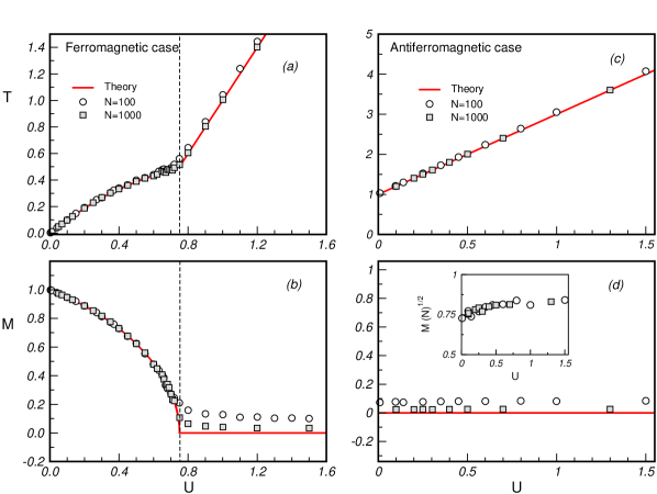
Figure 1: Temperature and magnetization as a function of the energy per particle $U$ for $A=0$ and $|\varepsilon|=1$ in the ferromagnetic (a),(b) and in the antiferromagnetic case (c),(d). Symbols refer to MD data for $N=10^{2}$ and $10^{3}$, while the solid lines refer to the canonical prediction obtained analytically in the mean-field limit. The vertical dashed line indicates the critical energy in the ferromagnetic model, located at $U_{c}=0.75$, $\beta_{c}=2$. The inset of panel (d) shows the rescaled magnetization $M\times\sqrt{N}$.

These results are confirmed by an analysis of the order parameter

$$M=\frac{I_{1}(\bar{y})}{I_{0}(\bar{y})}\quad.$$ (18)

For $\varepsilon>0$, the magnetization $M$ vanishes continuously at $\beta_{c}$ (see Fig. 1a,b), while it is always identical to zero in the antiferromagnetic case (see Fig. 1c,d). Since $M$ measures the degree of clustering of the particles, we have for $\varepsilon>0$ a transition from a clustered phase when $\beta>\beta_{c}$ to a homogeneous phase when $\beta<\beta_{c}$. We can obtain also the energy per particle

$$U=\frac{\partial(\beta f)}{\partial\beta}=\frac{1}{2\beta}+\frac{\varepsilon}{2}\left(1-M^{2}\right)$$ (19)

which is reported for $|\varepsilon|=1$ in Fig. 1. Panels (c) and (d) of Fig. 1 are limited to the range $U>0$ because in the antiferromagnetic model a non-homogeneous state, a bicluster, can be generated for smaller energies. The emergence of this state modifies all thermodynamical and dynamical features as will be discussed in section 4.2.

The dynamics of each particle obeys the following pendulum equation of motion

$$\ddot{\theta}_{i}=-M\sin(\theta_{i}-\phi)\quad,$$ (20)

where $M$ and $\phi$ have a non trivial time dependence, related to the motion of all the other particles in the system. Equation (20) has been very successfully used to describe several features of particle motion, like for instance trapping and untrapping mechanisms Antoni . There are also numerical indications Antoni and preliminary theoretical speculations priv that taking the mean-field limit before the infinite time limit, the time-dependence would disappear and the modulus and the phase of the magnetization become constant. This implies, as we will discuss in Section 5, that chaotic motion would disappear. The inversion of these two limits is also discussed in the contribution by Tsallis et al tsallisrap .

3.2 Canonical ensemble for $A\neq 0$

As soon as $A>0$, the evolution along the two spatial directions is no more decoupled and the system cannot be described in terms of a single order parameter. Throughout all this section $\epsilon=1$. A complete description of the phase diagram of the system requires now the introduction of two distinct order parameters:

$${\bf M}_{z}=\left(\frac{\sum_{i}\cos z_{i}}{N},\frac{\sum_{i}\sin z_{i}}{N}\right)=M_{z}\exp{(i\phi_{z})}$$ (21)

where $z_{i}=x_{i}$ or $y_{i}$ and;

$${\bf P}_{x\pm y}=\left(\frac{\sum_{i}\cos(x_{i}\pm y_{i})}{N},\frac{\sum_{i}\sin(x_{i}\pm y_{i})}{N}\right)=P_{z}\exp{(i\psi_{z})}\quad.$$ (22)

It can be shown that on average $M_{x}\simeq M_{y}\simeq M$ and $P_{x+y}\simeq P_{x-y}\simeq P$: therefore, we are left with only two order parameters.

Following the approach of section 3.1, the canonical equilibrium properties can be derived analytically in the mean-field limit at . We obtain

$$\beta f=\frac{M^{2}+P^{2}}{\beta}-\ln\left[\frac{G(M,P;A)}{\beta}\right]$$ (23)

with

$$G=\int_{0}^{2\pi}ds\enskip I_{0}\left(M+\sqrt{2A}P\cos s\right)\exp{(M\cos s)}$$ (24)

where $s$ is an integration variable.

The energy per particle reads as

$$U=\frac{1}{\beta}+\frac{2+A-2M^{2}-AP^{2}}{2}=K+V_{A}\quad.$$ (25)

Depending on the value of the coupling constant $A$, the single particle potential defined through $V_{A}=\frac{1}{2}\sum_{i}v_{i}$ changes its shape, inducing the different clustering phenomena described below. For small values of $A$, $v_{i}$ exhibits a single minimum per cell $(x,y)\in([-\pi,\pi],[-\pi,\pi])$ (see Fig. 2a for $A=1$), while for larger values of $A$ four minima can coexist in a single cell (see Fig. 2b for $A=4$). In the former case only one clustered equilibrium state can exist at low temperatures, while in the latter case, when all the four minima have the same depth a phase with two clusters can emerge, as described in the following.

Figure 2: Single particle potential $v_{i}(x,y)$ for $A=1,\varepsilon=1$ (a) and $A=4,\varepsilon=1$(b).

Since the system is ruled by two different order parameters $M$ and $P$, the phase diagram is more complicated than in the $A=0$ case and we observe two distinct clustered phases. In the very low temperature regime, the system is in the clustered phase $CP_{1}$: the particles have all the same location in a single point-like cluster and $M\approx P\approx 1$. In the very large temperature range, the system is in a homogeneous phase ($HP$) with particles uniformly distributed, $M\approx P=O(1/\sqrt{N})$. For $A>A_{2}\sim 3.5$, an intermediate two-clusters phase $CP_{2}$ appears. In this phase, due to the symmetric location of the two clusters in a cell, $M\sim O(1/\sqrt{N})$ while $P\sim O(1)$ art . We can gain good insights on the transitions by considering the line $T_{M}$ (resp. $T_{P}$) where $M$ (resp. $P$) vanishes and the phase $CP_{1}$ (resp. $CP_{2}$) looses its stability (see Fig. 3 for more details).

Figure 3: Canonical phase diagram of model (4) reporting the transition temperatures versus the coupling parameter $A$. The solid (resp. dashed) lines indicate the $T_{M}$ (resp. $T_{P}$) lines. The dots the points where the nature of the transitions change. $A_{1}$, $A_{2}$ and $A_{3}$ are the threshold coupling constants that determine the transition scenario $I\to IV$.

We can therefore identify the following four different scenarios depending on the value of $A$.

(I) When $0\leq A\leq A_{1}=2/5$, one observes a continuous transition from the phase $CP_{1}$ to $HP$. The critical line is located at $T_{M}=1/2$ ($U_{M}=3/2+A$) and a canonical tricritical point, located at $A_{1}=2/5$, separates the 1st order from the second order phase transition regions

(II) When $A_{1}<A<A_{2}\approx 3.5$, the transition between $CP_{1}$ and $HP$ is first order with a finite energy jump (latent heat). Inside this range of values of $A$ one also finds microcanonical discontinuous transitions (temperature jumps) as we will see in Section 3.2.

(III) When $A_{2}<A<A_{3}\approx 5.7$, the third phase begins to play a role and two successive transitions are observed: first $CP_{1}$ disappears at $T_{M}$ via a first order transition that gives rise to $CP_{2}$; then this two-clusters phase gives rise to the $HP$ phase via a continuous transition. The critical line associated to this transition is $T_{P}=A/4$ ($U_{P}=3A/4+1$).

(IV) When $A>A_{3}$, the transition connecting the two clustered phases, $CP_{1}$ and $CP_{2}$, becomes second order.

3.3 Microcanonical Ensemble

As we have anticipated, our microcanonical results have been mostly obtained via MD simulations, since we cannot estimate easily the microcanonical entropy $S$ analytically for the HMF model. However, we show below how far we can get, starting from the knowledge of the canonical free energy, using Legendre transform or inverse Laplace transform techniques. The following derivation is indeed valid in general, it does not refer to any specific microscopic model.

The relation that links the partition function $Z(\beta,N)$ to the microcanonical phase-space density at energy $E=U\cdot N$

$$\omega(E,N)=\int d^{N}p_{i}d^{N}\theta_{i}\;\delta(E-H)$$ (26)

is given by

$$Z(\beta,N)=\int_{0}^{\infty}dE\;\omega(E,N)\;{\rm e}^{-\beta E}~{},$$ (27)

where the lower limit of the integral ($E=0$) corresponds to the energy of the ground state of the model. Expression (27) can be readily rewritten as

$$Z(\beta,N)=N\int_{0}^{\infty}dU\exp{\left[N(-\beta U+\frac{1}{N}\ln(\omega(E,N))\right]}~{},$$ (28)

which is evaluated by employing the saddle-point technique in the mean-field limit. Employing the definition of entropy per particle in the thermodynamic limit

$$S(U)=\lim_{N\to\infty}\left[\frac{1}{N}\ln\omega(U,N)\right]\quad,$$ (29)

one can obtain the Legendre transform that relates the free energy to the entropy:

$$-\beta F(\beta)=\max_{U}[-\beta U+S(U)]\qquad{\rm with}\qquad\beta=\frac{\partial S}{\partial U}\quad.$$ (30)

Since a direct analytical evaluation of the entropy of the HMF model in the microcanonical ensemble is not possible, we are rather interested in obtaining the entropy from the free energy. This can be done only if the entropy $S$ is a concave function of the energy. Then, one can invert (30), getting

$$S(U)=\min_{\beta>0}[\beta(U-F(\beta))]\qquad{\rm with}\qquad U=\frac{\partial(\beta F)}{\partial\beta}\quad.$$ (31)

However, the assumption that $S$ is concave is not true for systems with long range interactions near a canonical first order transition, where a ”convex intruder” of $S$ appears BMRhmf ; grossdh , which gives rise to a negative specific heat regime in the microcanonical ensemble. For such cases, we have to rely on MD simulations or microcanonical Monte-Carlo simulations grossbook .

An alternative approach to the calculation of the entropy consists in expressing the Dirac $\delta$ function in Eq. (26) by a Laplace transform. One obtains

$$\omega(E,N)=\frac{1}{2i\pi}\int_{-i\infty}^{+i\infty}d\beta\;e^{\beta E}\;Z(\beta)$$ (32)

where one notices that $\beta$ is imaginary. As the partition function can be estimated for our model, we would just have to analytically continue to complex values of $\beta$. By performing a rotation to the real axis of the integration contour, one could then evaluate $\omega$ by saddle point techniques. However, this rotation requires the assumption that no singularity is present out of the real axis: this is not in general guaranteed. It has been checked numerically for the $A=0$ model barrethesis , allowing to obtain then an explicit expression for $\omega$ and confirming ensemble equivalence for this case.

However, when $A>A_{1}$, a first order canonical transition occurs, which implies the presence of a convex intruder and makes the evaluation of $S(U)$ through Eq. 31 impossible . For these cases, a canonical description is unable to capture all the features associated with the phase transition. For the microcanonical entropy, we have to rely here on MD simulations.

The MD simulations have been performed adopting extremely accurate symplectic integration schemes mac , with relative energy conservations during the runs of order $\sim 10^{-6}$. It is important to mention that the CPU time required by our integration schemes, due to the mean-field nature of the model, increases linearly with the number of particles.

Whenever we observe canonically continuous transitions (i.e. for $A\leq A_{1}$), the MD results coincide with those obtained analytically in the canonical ensemble, as shown in Fig. 1 for $A=0$. The curve $T(U)$ is thus well reproduced from MD data, apart from finite $N$ effects. It has been however observed that starting from ”water-bags” initial conditions metastable states can occur in the proximity of the transition tsallisrap .

Figure 4: Temperature-energy relation in the coexistence region for A=1 (a) and A=4 (b). Lines indicate canonical analytical results, while circles correspond to microcanonical MD simulations. Solid thick lines are equilibrium results, solid thin lines metastable states and dashed thin lines unstable states. The dash-dotted line is the Maxwell construction. Figure (a) refers to a first order transition from $CP_{1}$ to $HP$, (b) to discontinuous transition connecting the two clustered phases. In (b) the second order transition from $CP_{2}$ to $HP$ associated to the vanishing of $P$ is also shown. The MD results refer to model (4) with $N=5000$ averaged over a time $t=10^{6}$.

When $A>A_{1}$, discrepancies between the results obtained in the two ensembles are observable in Fig. 4. For example, MD results in the case $A=1$, reported in Fig. 4(a), differ clearly from canonical ones around the transition, exhibiting a regime characterized by a negative specific heat. This feature is common to many models with long-range thir ; compa or power-law decaying interactions tamahmf as well as to finite systems with short-range forces grossbook . However, only recently a characterization of all possible microcanonical transitions associated to canonically first order ones has been initiated BMRhmf ; art .

For $A$ slightly above $A_{1}$, the transition is microcanonically continuous, i.e. there is no discontinuity in the $T-U$ relation (this regime presumably extends up to $A\sim 1.2$). Before the transition, one observes a negative specific heat regime (see Fig. 4a). In addition, as already observed for the Blume-Emery-Griffiths model BMRhmf , microcanonically discontinuous transitions can be observed in the ”convex intruder” region. This means that, at the transition energy, temperature jumps exist in the thermodynamic limit. A complete physical understanding of this phenomenon, which has also been found in gravitational systems chavanishmf , has not been reached. For $A>1.2$, i.e. above the ”microcanonical tricritical point”, our model displays temperature jumps. This situations is shown in Fig. 5 for $A=2$.

Figure 5: Evolution of the temperature $T$ versus the energy $U$ in the case $A=2$. The symbols refer to MD results obtained by successively cooling or warming a certain initial configuration. Each simulation has been performed at constant total energy and refers to a system of $N=4,000$ particles integrated for a time $t=10^{6}$. The solid lines are computed in the canonical ensemble and include also unstable and metastable cases. The solid vertical line indicating the transition energy has been estimated via a Maxwell construction performed in the microcanonical ensemble (for details see BMRhmf ).

For $A>A_{2}$, we have again a continuous transition connecting the two clustered phases $CP_{1}$ and $CP_{2}$. This is the first angular point in the $T-U$ relation at $U\sim 3.65$ in Fig. 4(b). The second angular point at $U\sim 4$ is the continuous transition, connecting $CP_{2}$ to $HP$. The transition at lower energy associated to the vanishing of $M$ is continuous in the microcanonical ensemble with a negative specific heat, while discontinuous in the canonical ensemble; the dash-dotted line indicates the transition temperature in the canonical ensemble, derived using the Maxwell construction). The second transition associated to the vanishing of $P$ is continuous in both ensembles.

4 Dynamical Properties I: Out-of-equilibrium states

4.1 Metastable states

Around the critical energy, relaxation to equilibrium depends in a very sensitive way on the initial conditions adopted. When one starts with out-of-equilibrium initial conditions in the ferromagnetic case, one finds quasi-stationary (i.e. long lived) nonequilibrium states. An example is represented by the so-called “water bag” initial condition: all the particles are clustered in a single point and the momenta are distributed according to a flat distribution of finite width centered around zero. These states have a lifetime which increases with the number of particles $N$, and are therefore stationary in the continuum limit. In correspondence of these metastable states, anomalous diffusion and Lévy walks levyhmf , long living correlations in $\mu-$space lat0 and zero Lyapunov exponents lat0a have been found. In addition, these states are far from the equilibrium caloric curve around the critical energy, showing a region of negative specific heat and a continuation of the high temperature phase (linear $T$ vs $U$ relation) into the low temperature one. It is very intriguing that these out-of-equilibrium quasi-stationary states indicate a caloric curve very similar to the one found in the region where one gets a canonical first order phase transitions, but a continuous microcanonical one, as discussed in section 3.3. In the latter case, however, the corresponding states are stationary also at finite $N$. The coexistence of different states in the continuum limit near the critical region is a purely microcanonical effect, and arises after the inversion of the $t\to\infty$ limit with the $N\to\infty$ one lat0 ; lat0a ; tsallisrap .

Similarly, the antiferromagnetic HMF ($A=0$, $\varepsilon=-1$), where the particles interact through repulsive forces presents unexpected dynamical properties in the out-of-equilibrium thermodynamics. On the first sight, the thermodynamics of this model seems to be less interesting since no phase transition occurs as discussed above. However, thermodynamical predictions are again in some cases in complete disagreement with dynamical results leading in particular to a striking localization of energy. This aspect, as we will show below, is of course, again, closely related to the long-range character of the interaction and to the fact that such a dynamics is chaotic and self-consistent. We mean by this that all particles give a contribution to the field acting on each of them. One calls this phenomenon, self-consistent chaos Diego . In addition to the toy model that we consider here, we do think that similar emergence of structures, but even more importantly, similar dynamical stabilization of out-equilibrium states could be encountered in other long-range systems, as we briefly describe at the end of this section.

4.2 The dynamical emergence of the bicluster in the antiferromagnetic case

In the antiferromagnetic case, Eq. (7) with $\varepsilon=-1$, the intriguing properties appear in the region of very small energies. To be more specific, if an initial state with particles evenly distributed on the circle (i.e. close to the ground state predicted by microcanonical or canonical thermodynamics) and with vanishingly small momenta is prepared, this initial condition can lead to the formation of unstable states. This process, discovered by chance, is now characterized in full detail Antoni ; barreepjB ; drh ; firpoleyvraz .

As shown by Fig. 6, the density of particles is initially homogeneous. However a localization of particles do appear at a given time, in two different points, symmetrically located with respect to the center of the circle. This localized state, that we call bicluster, is however unstable (as shown again by Fig. 6), since both clusters are giving rise to two smaller localized groups of particles: this is the reason for the appearance of the first chevron. However, also this state is unstable, so that the first chevron disappears to give rise again to a localization of energy in two points. This state enhances the formation of a chevron with a smaller width and this phenomenon repeats until the width of the chevron is so small that one does not distinguish anymore its destabilization. Asymptotically one gets a density distribution displaying two sharp peaks located at distance $\pi$ on the circle, a dynamically stable bicluster.

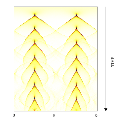
Figure 6: Short-time evolution of the particle density in grey scale: the darker the grey, the higher the density. Starting from an initial condition with all the particles evenly distributed on the circle, one observes a very rapid concentration of particles, followed by the quasi periodic appearance of chevrons, that shrink as time increases.

As we have shown in Ref. barreepjB , the emergence of the bicluster is the signature of shock waves present in the associated hydrodynamical equations. Indeed, we found a strikingly good description of the dynamics of the particles by a non linear analysis of the associated Vlasov equation, which is mathematically justified BraunHepp in the infinite $N$ limit. The physical explanation of this problem can be summarized as follows. Once the Hamiltonian has been mapped to the Vlasov equation, it is possible to introduce a density $\rho(\theta,t)$ and a velocity field $v(\theta,t)$. Neglecting the dispersion in momentum and relying on usual non linear dynamics hierarchy of time-scales, one ends up with dynamical equations at different orders in a multiscale analysis. The first order corresponds to the linear dynamics and defines the plasma frequency of order one. However, a second timescale appears that is related to the previous one by the relationship $\tau=\sqrt{U}\,t$, where $U$ is the energy per particle. When one considers initial conditions with a very small energy density, the two time scales are very different and clearly distinguishable by considering particle trajectories: a typical trajectory corresponds indeed to a very fast motion with a very small amplitude, superimposed to a slow motion with a large amplitude.

This suggests to average over the fast oscillations and leads to the spatially forced Burgers equation

$$\frac{\partial u}{\partial\tau}+u\frac{\partial u}{\partial\theta} = -\frac{1}{2}\sin 2\theta\qquad,$$ (33)

once the average velocity $u(\theta,\tau)=\langle v(\theta,t,\tau)\rangle_{t}$ is introduced. Due to the absence of dissipative or diffusive terms, Equation (33) supports shock waves and these can be related to the emergence of the bicluster. By applying the methods of characteristics to solve Equation (33), one obtains

$$\frac{d^{2}\theta}{d\tau^{2}}+\frac{1}{2}\sin 2\theta = 0\;.$$ (34)

which is a pendulum-like equation.

Fig. 7 shows the trajectories, derived from Eq. (34), for particles that are initially evenly distributed on the circle. One clearly sees that two shock waves appear and lead to an increase of the number of particles around two particular sites, which depend on the initial conditions: this two sites correspond to the nucleation sites of the bicluster. Because of the absence of a diffusive term, the shock wave starts a spiral motion that explains the destabilization of the first bicluster and also the existence of the two arms per cluster, i.e. the chevron.

Figure 7: Five successive snapshots of the velocity profiles $u(\theta,t)$ are shown including the initial state when all particles are uniformly distributed in space with a small velocity dispersion.

This dynamical analysis allows an even more precise description, since the methods of characteristics show that the trajectories correspond to the motion of particles in the double well periodic potential $V(\theta,\tau)=-(\cos 2\theta)/4$. This potential is of mean field origin, since it represents the effect of all interacting particles. Therefore, the particles will have an oscillatory motion in one of the two wells. One understands thus that particles starting close to the minimum will collapse at the same time, whereas a particle starting farther will have a larger oscillation period. This is what is shown in Fig. 8 where trajectories are presented for different starting positions. One sees that the period of recurrence of the chevrons corresponds to half the period of oscillations of the particles close to the minimum; this fact is a direct consequence of the isochronism of the approximate harmonic potential close to the minimum. The description could even go one step further by computing the caustics, corresponding to the envelops of the characteristics. They are shown in Fig. 8 and testify the striking agreement between this description and the real trajectories: the chevrons of Fig. 6 correspond to the caustics.

Figure 8: Superposition of the caustics (thick full lines) over the characteristics (dotted lines) of particles that are initially evenly distributed between $-\pi/2$ and $\pi/2$.

4.3 Thermodynamical predictions versus dynamical stabilization

If the above description is shown to be particularly accurate, it does not explain why this state is thermodynamically preferred over others. Indeed, as shown before, thermodynamics predicts that the only equilibrium state is homogeneous. This result has been discussed in Section 3.1, where we have proved that magnetization is zero at all energies for the antiferromagnetic model and this has been also confirmed by Monte Carlo simulations drh . However, since MD simulations are performed at constant energy, it is important to derive analytically the most probable state in the microcanonical ensemble. Since this model does not present ensemble inequivalence, we can obtain the microcanonical results by employing the inverse Laplace transform (32) of the canonical partition function. The microcanonical solution confirms that the maximal entropy state is homogeneous on the circle. It is therefore essential to see why the bicluster state, predicted to be thermodynamically unstable is instead dynamically stable.

The underlying reason rely on the existence of the two very different timescales and the idea is again to average over the very fast one. Instead of using the classical asymptotic expansion on the equation of motions, it is much more appropriate to develop an adiabatic approximation which leads to an effective Hamiltonian that describes very well the long time dynamics. Doing statistical mechanics of this averaged problem, one predicts the presence of the bicluter.

The theory that we have developed relies on an application of adiabatic theory, which in the case of the HMF model is rather elaborate and needs lengthy calculations barreepjB that we will not present here. An alternative, but less powerful, method to derive similar results has been used in Ref. firpoleyvraz . On the contrary, we would like to present a qualitative explanations of this phenomenon, using a nice (but even too simple !) analogy.

This stabilization of unstable states can be described using the analogy with the inverted pendulum, where the vertical unstable equilibrium position can be made stable by the application of a small oscillating force. One considers a rigid rod free to rotate in a vertical plane and whose point-of-support is vibrated vertically as shown by Fig. 9a. If the support oscillates vertically above a certain frequency, one discovers the remarkable property that the vertical position with the center of mass above its support point is stable (Fig. 9b). This problem, discussed initially by Kapitza Kapitaza , has strong similarities with the present problem and allows a very simplified presentation of the averaging technique we have used.

Figure 9: Schematic picture of the inverted pendulum.

The equation of motion of the vibrating pendulum is

$$\frac{d^{2}\theta}{dt^{2}}+\left(\frac{\omega_{0}^{2}}{\omega^{2}}-a\cos t\right)\sin\theta=0~{},$$ (35)

where $\omega_{0}$ is the proper linear frequency of the pendulum, $\omega$ the driving frequency of the support and $a$ the amplitude of excitation. Introducing a small parameter $\varepsilon=\omega_{0}/\omega$, one sees that (35) derives from the Lagrangian

$${\cal L}=\frac{1}{2}\left(\frac{d\theta}{dt}\right)^{2}+\left(\varepsilon^{2}-a\cos t\right)\cos\theta\quad.$$ (36)

Here the two frequencies $\omega$ and $\omega_{0}$ define two different time scales, in close analogy with the HMF model. Using the small parameter to renormalize the amplitude of the excitation as $A=a/\varepsilon$, and choosing the ansatz $\theta=\theta_{0}(\tau)+\varepsilon\,\theta_{1}(t,\varepsilon)$ where $\tau=\varepsilon t$, the Lagrangian equations for the function $\theta_{1}$, leads to the solution $\theta_{1}=-A\cos t\sin\theta_{0}(\tau)$. This result not only simplifies the above ansatz, but more importantly suggest to average the Lagrangian on the fast variable $t$ to obtain an effective Lagrangian ${\cal L}_{eff}=\langle{\cal L}\rangle_{t}=\frac{1}{2}\left(\frac{d\theta_{0}}{d\tau}\right)^{2}+V_{eff}$ , where the averaged potential is found to be

$$V_{eff}=-\cos\theta_{0}-\frac{A^{2}}{8}\cos 2\theta_{0}+\mbox{Cste}\quad.$$ (37)

It is now straightforward to show that the inverted position would be stable if $A^{2}>2$, i.e. if $a\omega>\sqrt{2}\omega_{0}$. As the excitation amplitude $a$ is usually small, this condition emphasizes that the two time scales should be clearly different, for the inverted position to be stable.

The procedure for the HMF model is analogous, but of course it implies a series of tedious calculations. Since we would like to limit here to a pedagogical presentation, we will skip such details that can be found in Ref. barreepjB . It is however important to emphasize that the potential energy in the HMF model is self-consistently determined and depend on the position of all particles. The magic and the beauty is that, even if this is the potential energy of $N$ particles, it is possible to compute the statistical mechanics of the new effective Hamiltonian, derived directly from the effective Lagrangian via the Legendre transform. The main result is that the out-of-equilibrium state, (i.e. the bicluster shown in Fig. 6) corresponds to a statistical equilibrium of the effective mean-field dynamics. No external drive is present in this case, as for the inverted pendulum, but the time dependence of the mean field plays the role of the external drive.

The HMF model represents presumably the simplest $N$-body system where out-of-equilibrium dynamically stabilized states can be observed and explained in detail. However, we believe that several systems with long range interactions should exhibit behaviours similar to the ones we have observed here. Moreover, this model represents a paradigmatic example for other systems exhibiting nonlinear interactions of rapid oscillations and a slower global motion. One of this is the piston problem piston : averaging techniques have been applied to the fast motion of gas particles in a piston which itself has a slow motion sinairusse . Examples can also be found in applied physics as for instance wave-particles interaction in plasma physics plasma , or the interaction of fast inertia gravity waves with the vortical motion for the rotating Shallow Water model embidmajda .

5 Dynamical Properties II: Lyapunov exponents

In this section, we discuss the chaotic features of the microscopic dynamics of the HMF model. We mainly concentrate on the $A=0$ case, presenting in details the behavior of the Lyapunov exponents and the Kolmogorov-Sinai entropy both for ferromagnetic and antiferromagnetic interactions. We also briefly discuss some peculiar mechanisms of chaos in the $A\neq 0$ case. The original motivation for the study of the chaotic properties of the HMF was to investigate the relation between phase transitions, which are macroscopic phenomena, and microscopic dynamics (see Ref. laporeport for a review) with the purpose of finding dynamical signatures of phase transitions cmd . Moreover, we wanted to check the scaling properties with the number of particles of the Lyapunov spectrum livipolruffo in the presence of long-range interactions.

5.1 The $A=0$ case

In the $A=0$ case (see formulae (7)-(20)), the Hamiltonian equations of motion are

$$\dot{\theta}_{i} = p_{i}$$ (38)

$$\dot{p}_{i} = -M\sin\left(\theta_{i}-\phi\right)\quad.$$ (39)

The Largest Lyapunov Exponent (LLE) is defined as the limit

$${\lambda_{1}}=\lim_{t\to\infty}{1\over t}\ln{d(t)\over d(0)}$$ (40)

where $d(t)=\sqrt{\sum_{i=1}^{N}(\delta\theta_{i})^{2}+(\delta p_{i})^{2}}$ is the Euclidean norm of the infinitesimal disturbance at time $t$. Therefore, in order to obtain the time evolution of $d(t)$, one has to integrate also the linearized equations of motion along the reference orbit

$${d\over dt}\delta\theta_{i}=\delta p_{i}~{}~{}~{}~{},~{}~{}~{}~{}{d\over dt}\delta p_{i}~{}=-\sum_{j}{{\partial^{2}V}\over{\partial\theta_{i}\partial\theta_{j}}}\delta q_{j}~{}~{},$$ (41)

where the diagonal and off-diagonal terms of the Hessian are

$${\partial^{2}V\over{\partial\theta_{i}^{2}}} = M\cos(\theta_{i}-\Phi)-\frac{1}{N}$$ (42)

$${{\partial^{2}V}\over{\partial\theta_{i}\partial\theta_{j}}} = -{1\over{N}}\cos(\theta_{i}-\theta_{j})\quad,~{}~{}~{}i\neq j~{}~{}.$$ (43)

To calculate the largest Lyapunov exponent we have used the standard method by Benettin et al ben . In Fig. (10), we report the results obtained for four different sizes of the system (ranging from $N=100$ to $N=20,000$).

In panel (a), we plot the largest Lyapunov exponent as a function of U. As expected, $\lambda_{1}$ vanishes in the limit of very small and very large energies, where the system is quasi-integrable. Indeed, the Hamiltonian reduces to weakly coupled harmonic oscillators in the former case or to free rotators in the latter. For $U<0.2$, $\lambda_{1}$ is small and has no $N$-dependence. Then it changes abruptly and a region of “strong chaos” begins. It was observed Antoni that between $U=0.2$ and $U=0.3$, a different dynamical regime sets in and particles start to evaporate from the main cluster, in analogy with what was reported in other models cmd ; nayak . In the region of strong chaoticity, we observe a pronounced peak already for $N=100$ yama . The peak persists and becomes broader for $N=20,000$. The location of the peak is slightly below the critical energy and depends weakly on $N$.

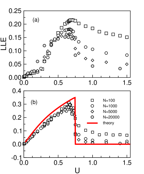
Figure 10: Largest Lyapunov exponent LLE and kinetic energy fluctuations $\Sigma=\sigma_{K}/\sqrt{N}$ as a function of U in the $A=0$ ferromagnetic case for different N sizes. The theoretical curve is shown as a full line, see text.

In panel (b), we report the standard deviation of the kinetic energy per particle $\Sigma$ computed from

$$\Sigma=\frac{\sigma_{K}}{\sqrt{N}}={{\sqrt{\langle K^{2}\rangle-\langle K\rangle^{2}}}\over\sqrt{N}}\quad,$$ (44)

where $\langle\bullet\rangle$ indicates the time average. The theoretical prediction for $\Sigma$, which is also reported in Fig.10, is firpo ; lat2hmf

$$\Sigma={T\over\sqrt{2}}\sqrt{1-{\left[1-2M\left({dM\over dT}\right)\right]}^{-1}}\quad,$$ (45)

where $M(T)$ is computed in the canonical ensemble. Finite size effects are also present for the kinetic energy fluctuations, especially for $U>U_{c}$, but in general there is a good agreement with the theoretical formula, although the experimental points in Fig. 10b lies systematically below it. The figure emphasizes that the behavior of the Lyapunov exponent is strikingly correlated with $\Sigma$: in correspondence to the peak in the LLE, we observe also a sharp maximum of the kinetic energy fluctuations. The relation between the chaotic properties and the thermodynamics of the system, namely the presence of a critical point, can be made even more quantitative. An analytical formula, relating (in the $A=0$ model) the LLE to the second order phase transition undergone by the system, has been obtained firpo by means of the geometrical approach developed in Refs. lapo1 ; laporeport . Using a reformulation of Hamiltonian dynamics in the language of Riemannian geometry, they have found a general analytical expression for the LLE of a Hamiltonian many-body system in terms of two quantities: the average $\Omega_{0}$ and the variance $\sigma_{\Omega}$ of the Ricci curvature $\kappa_{R}=\Delta V/N=1/N~{}\sum_{i=1}^{N}{\partial^{2}V\over{\partial q_{i}^{2}}}$, where $V$ is the potential energy and $q_{i}$ are the coordinates of the system. Since in the particular case of the HMF model, we have

$${1\over N}\sum_{i=1}^{N}{\partial^{2}V\over{\partial\theta_{i}^{2}}}=M^{2}-{1\over N}={2K\over N}+1-2U-{1\over N}~{}~{},$$ (46)

the two quantities $\Omega_{0}$ and $\sigma_{\Omega}$ can be expressed in terms of average values and fluctuations either of $M^{2}$ or of the kinetic energy $K$

$$\Omega_{0} = \langle M^{2}\rangle-\frac{1}{N}=\frac{2}{N}\langle K\rangle+(1-2U)-\frac{1}{N}$$ (47)

$$\sigma^{2}_{\Omega} = N{\sigma^{2}_{M^{2}}}=\frac{4}{N}{\sigma^{2}_{K}~{}~{}.}$$ (48)

The formula obtained by Firpo firpo relates the LLE, a characteristic dynamical quantity, to thermodynamical quantities like $\langle M^{2}\rangle$ and ${\sigma_{M^{2}}}$, or $\langle K\rangle$ and ${\sigma_{K}}$, which characterize the macroscopic phase transition. For moderately small values of $U$, an approximation of the formula gives

$$\lambda\propto\frac{\sigma_{K}}{\sqrt{N}}=\Sigma~{}~{}.$$ (49)

This is in agreement with the proportionality between LLE and fluctuations of the kinetic energy found numerically in Fig. (10). This implies also a connection between the LLE and the specific heat, another quantity which is directly related to the kinetic energy fluctuation. In fact the specific heat can be obtained from $\Sigma$ by means of the Lebowitz-Percus-Verlet formula lpv

$$C_{V}={1\over 2}\left[1-2\left({\Sigma\over T}\right)^{2}\right]^{-1}\quad.$$ (50)

In Fig. 11, we report the numerical results for the specific heat as a function of $U$ for a system made of $N=500$ particles, and we compare them with the theoretical estimate.

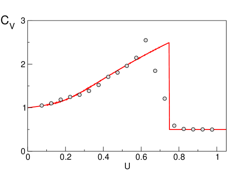
Figure 11: Specific heat as a function of U in the $A=0$ ferromagnetic case. The numerical simulation at equilibrium for a system with $N=500$ is compared with the expected theoretical result (50).

In the HMF model and for a rather moderate size of the systems, it is possible to calculate not only the LLE but all the Lyapunov exponents, and from them the Kolmogorov-Sinai entropy. We give first a succinct definition of the spectrum of Lyapunov exponents (for more details see Ruelleeckman ). Once the 2N-dimensional tangent vector ${\bf z}=(\delta\theta_{1},\cdots,\delta\theta_{N},\delta p_{1},\cdots,\delta p_{N})$ is defined, with its dynamics given by Eqs. (41), one can formally integrate the motion in tangent space up to time $t$, since the equations are linear,

$${\bf z}(t)=J^{t}{\bf z}(0)~{},$$ (51)

where $J^{t}$ is a $2N\times 2N$ matrix that depends on time through the orbit $\theta_{i}(t),p_{i}(t)$. The first $k$ exponents of the spectrum $\lambda_{1},\dots,\lambda_{k}$, which are ordered from the maximal to the minimal, are then given by

$$(\lambda_{1}+\dots+\lambda_{k})=\lim_{t\to\infty}\frac{1}{2t}\ln\mbox{Tr}J_{k}^{t}(J_{k}^{t})^{*}\quad,$$ (52)

where $J_{k}^{t}$ is the matrix ($(J_{k}^{t})^{*}$ its transpose) induced by $J^{t}$ that acts on the exterior product of $k$ vectors in the tangent space ${\bf z}_{1}\land\dots\land{\bf z}_{k}$. The spectrum extends up to $k=2N$ and in our Hamiltonian system obeys the pairing rule

$$\lambda_{i}=-\lambda_{2N+1-i}\quad\mbox{for}\quad 1\leq i\leq 2N~{}.$$ (53)

The numerical evaluation of the spectrum of the Lyapunov exponents is a heavy computational task, in particular for the necessity to perform Gram-Schmidt orthonormalizations of the Lyapunov eigenvectors in order to maintain them mutually orthogonal during the time evolution. We have been able to compute the complete Lyapunov spectrum for system sizes up to $N=100$. In Fig. 12, we report the positive part of the spectrum for different system sizes and an energy $U=0.1$ inside the weakly chaotic region. The negative part of the spectrum is symmetric due to the pairing rule (53). The limit distribution $\lambda(x)$, suggested for short range interactions,

$$\lambda(x)=\lim_{N\to\infty}\lambda_{xN}(N)~{},$$ (54)

that is obtained by plotting $\lambda_{i}$ vs. $i/N$ and letting $N$ going to infinity, is found also here for the $N$ values that we have been able to explore. At higher energies, this scaling is not valid and a size-dependence is present lat2hmf .

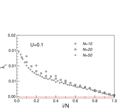
Figure 12: Scaling of the positive part of the spectrum of Lyapunov exponents in the A=0 ferromagnetic case for $U=0.1$.

The Kolmogorov-Sinai (K-S) entropy is, according to Pesin’s formula Ruelleeckman , the sum of the positive Lyapunov exponents. In Fig. 13, we plot the entropy density $S_{KS}/N$ as a function of $U$ for different systems sizes.

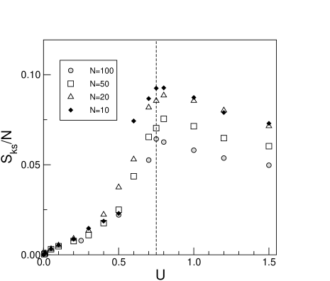
Figure 13: $S_{KS}/N$ as a function of $U$ in the $A=0$ ferromagnetic case.Numerical calculations for different systems sizes ranging from $N=10$ to $N=100$ are shown. The dashed line indicates the critical energy.

As for the LLE, $S_{KS}/N$ shows a peak near the critical energy, a fast convergence to a limiting value as $N$ increases in the small energy limit, and a slow convergence to zero for $U\geq U_{c}$. A comparison of the ferromagnetic and antiferromagnetic cases is reported in Fig. 14.

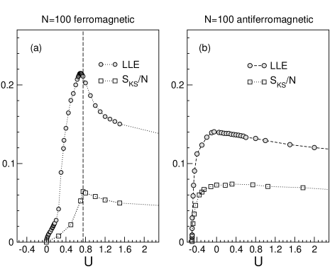
Figure 14: LLE and $S_{KS}/N$ as a function of $U$ in the $A=0$ ferromagnetic and antiferromagnetic cases for N=100.

Here, for N=100, we plot as a function of $U$ the LLE and the Kolmogorov-Sinai entropy per particle $S_{KS}/N$. In both the ferromagnetic and antiferromagnetic cases, the system is integrable in the limits of small and large energies. The main difference between the ferromagnetic and the antiferromagnetic model appears at intermediate energies. In fact, although both cases are chaotic (LLE and $S_{KS}/N$ are positive), in the ferromagnetic system one observes a well defined peak just below the critical energy, because the dynamics feels the presence of the phase transition. On the other hand, a smoother curve is observed in the antiferromagnetic case.

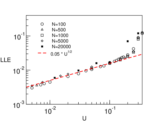
Figure 15: Scaling properties of the LLE at low energies in the $A=0$ ferromagnetic case. No N-dependence is observed for $U<0.2$. The dashed line indicates a power-law $U^{1/2}$.

In the low energy regime, it is possible to work out lat1hmf a simple estimate $\lambda_{1}\propto\sqrt{U}$, which is fully confirmed for the ferromagnetic case in Fig. 15 for different system sizes in the range $N=100,20000$. The same scaling law is also valid in the antiferromagnetic case latoraprogtherophys and for the $A=1$ at HMF model.

At variance with the $N$-independent behavior observed at small energy, strong finite size effects are present above the critical energy in the ferromagnetic case and for all energies for the antiferromagnetic case. In Fig. 16(a), we show that the LLE is positive and $N$-independent below the transition (see the values $U=0.4,0.5$), while it goes to zero with $N$ above. We also report in the same figure a calculation of the LLE using a random distribution of particle positions $\theta_{i}$ on the circle in Eq. (41) for the tangent vector. The agreement between the deterministic estimate and this random matrix calculation is very good. The LLE scales as $N^{-{1\over 3}}$, as indicated by the fit reported in the figure. This agreement can be explained by means of an analytical result obtained for the LLE of product of random matrices pari . If the elements of the symplectic random matrix have zero mean, the LLE scales with the power $2/3$ of the perturbation. In our case, the latter condition is satisfied and the perturbation is the magnetization $M$. Since $M$ scales as $N^{-{1\over 2}}$, we get the right scaling of $\lambda_{1}$ with $N$. This proves that the system is integrable for $U\geq U_{c}$ as $N\to\infty$. This result is also confirmed by the analytical calculations of Ref. firpo and, more recently, of Ref. Vallejos .

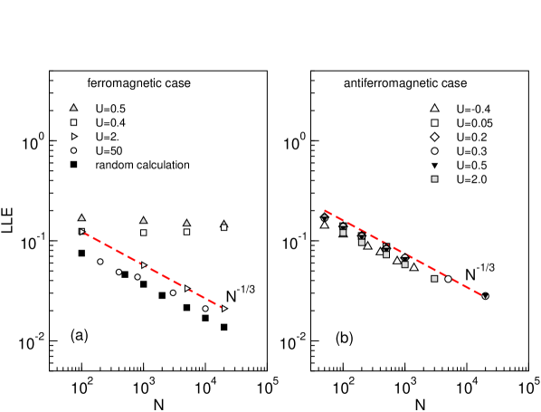
Figure 16: Scaling of the LLE vs $N$ for the $A=0$ ferromagnetic and antiferromagnetic cases at various energies, see text. A power-law decreasing as $N^{-1/3}$ of the LLE is observed for overcritical energies in the ferromagnetic case and for all energies in the antiferromagnetic one. See text for further details.

In the antiferromagnetic case, the LLE goes to zero with system size as $N^{-{1\over 3}}$ for all values of $U$.

Interesting scaling laws have also been found for the Kolmogorov-Sinai entropy in the ferromagnetic case: at small energies $S_{KS}/N\propto U^{3/4}$ with no size dependence, and $S_{KS}/N\propto N^{-1/5}$ for overcritical energy densities. The latter behavior has been found also in other models tsuchia . Concluding this section we would like to stress that the finite value of chaotic measures close to the critical point is strongly related to kinetic energy fluctuations and can be considered as a microscopic dynamical indication of the macroscopic equilibrium phase transition. This connection has been found also in other models and seems to be quite general laporeport ; cmd ; lapo3 ; barrehmf

The behavior of the HMF model as a function of the range of the interaction celiahmf ; tamahmf ; campa and the dynamical features before equilibration lat0 ; lat0a is discussed in a separate chapter of this volume in connection to Tsallis nonextensive thermodynamics tsallisrap .

5.2 Mechanisms of chaos in the $A\neq 0$ case

For $A=0$, the origin of chaos is related to the non time-dependence of Eq. (20), since it is obvious that if the phase $\phi$ and the magnetization $M$ would become constant the dynamics of the system will reduce to that of an integrable system. There are indeed preliminary indications priv that in the mean-field limit $N\to\infty$, $M$ and $\phi$ will become constant and $\lambda\to 0$ . It should be noticed that this is true if the mean-field limit is taken before the limit $t\to\infty$ in the definition of the maximal Lyapunov exponent, and numerical indications were reported in Ref. lat0a . When $A>0$ we expect a quite different situation: indeed, even assuming that in the mean-field limit $M$ and $P$ and their respective phases will become constant, the dynamics will eventually take place in a $4$-dimensional phase space and chaos can in principle be observed.

As already shown in at , for $A=1$ and $\varepsilon=1$, two different mechanisms of chaos are present in the system for $U<U_{c}$ : one acting on the particles trapped in the potential and another one felt by the particles moving in proximity of the separatrix. This second mechanism is well known and is related to the presence of a chaotic layer situated around the separatrix. The origin of the first mechanism is less clear, but presumably related to the erratic motion of the minimum of the potential well, i.e. to the time-dependent character of the equations ruling the dynamics of the single particle. Indications in this direction can be found by performing the following numerical experiment. Let us prepare a system with $N=200$ and $U=0.87$ (the critical energy is in this case $U_{c}\sim 2$) with a Maxwellian velocity distribution and with all particles in a single cluster.

For an integration time $t<2\times 10^{6}$, the Lyapunov exponent has a value $\lambda\simeq 0.13$. But when at time $t\sim 2\times 10^{6}$, one particle escapes from the cluster, its value almost doubles (see Fig. 17). The escaping of the particle from the cluster is associated to a decrease of the magnetization $M$ and of the kinetic energy $K$. This last effect is related to the negative specific heat regime: the potential energy $V_{A}$ is minimal when all the particles are trapped, if one escapes then $V_{A}$ increases and due to the energy conservation $K$ decreases. As a matter of fact, we can identify a “strong” chaos felt from the particles approaching the separatrix and a “weak” chaos associated to the orbits trapped in the potential well. We believe that the latter mechanism of chaotization should disappear (in analogy with the $A=0$ case) when the mean-field limit is taken before the $t\to\infty$ limit. Therefore we expect that for $N\to\infty$ the only source of chaotic behaviour should be related to the chaotic sea located around the separatrix. As already noticed in Ref. at , the degree of chaotization of a given system depends strongly on the initial condition (in particular in the mean-field limit). In the latter limit, for initial condition prepared in a clustered configuration, we expect that $\lambda=0$, until one particle will escape from the cluster.

Figure 17: Time evolution of the Largest Lyapunov Exponent (LLE) $\lambda_{1}$, of the magnetization $M$, and of the kinetic energy $K$ are shown for a clustered initial condition for the model with $A=1$ and $\varepsilon=1$ at $U=0.87$ and with $N=200$.

6 Conclusions

We have discussed the dynamical properties of the Hamiltonian Mean Field model in connection to ita thermodynamics. This apparently simple class of models has revealed a very rich and interesting variety of behaviours. Inequivalence of ensembles, negative specific heat, metastable dynamical states and chaotic dynamics are only some among them. During the past years these models have been of great help in understanding the connection between dynamics and thermodynamics when long-range interactions are present. Such kind of investigation is of extreme importance for self-gravitating systems and plasmas, but also for phase transitions in finite systems, such as atomic clusters or nuclei, and for the foundation of statistical mechanics. Several progresses have been done during these years. This contribution, although not exhaustive, is an effort to summarize some of the main results achieved so far. We believe that the problems which are still not understood will be hopefully clarified in the near future within a general theoretical framework. We list three important open questions that we believe can be reasonably addresses: the exact solution of the model in the microcanonical ensemble; the full characterization of the out-of-equilibrium states close to phase transitions; the clarification of the scaling laws of the maximal Lyapunov exponent and of the Lyapunov spectrum; the study of the single-particle diffusive motion levyhmf in the various non-equilibrium and equilibrium regimes.

References

- (1) T. Padhmanaban, Statistical Mechanics of gravitating systems in static and cosmological backgrounds, in “Dynamics and Thermodynamics of Systems with Long Range Interactions”, T. Dauxois, S. Ruffo, E. Arimondo, M. Wilkens Eds., Lecture Notes in Physics Vol. 602, Springer (2002), (in this volume)
- (2) P.-H. Chavanis, Statistical mechanics of two-dimensional vortices and stellar systems, in “Dynamics and Thermodynamics of Systems with Long Range Interactions”, T. Dauxois, S. Ruffo, E. Arimondo, M. Wilkens Eds., Lecture Notes in Physics Vol. 602, Springer (2002), (in this volume)
- (3) Elskens, Kinetic theory for plasmas and wave-particle hamiltonian dynamics, in “Dynamics and Thermodynamics of Systems with Long Range Interactions”, T. Dauxois, S. Ruffo, E. Arimondo, M. Wilkens Eds., Lecture Notes in Physics Vol. 602, Springer (2002), (in this volume)
- (4) F. Tamarit and C. Anteneodo, Physical Review Letters 84, 208 (2000)
- (5) J. Barré, D. Mukamel, S. Ruffo, Ensemble inequivalence in mean-field models of magnetism, in “Dynamics and Thermodynamics of Systems with Long Range Interactions”, T. Dauxois, S. Ruffo, E. Arimondo, M. Wilkens Eds., Lecture Notes in Physics Vol. 602, Springer (2002), (in this volume)
- (6) A. Campa, A. Giansanti, D. Moroni, Physical Review E 62, 303 (2000) and Chaos Solitons and Fractals 13, 407 (2002)
- (7) J.-P. Eckmann, D. Ruelle, Review of Modern Physics 57, 615 (1985)
- (8) S. Ruffo, in Transport and Plasma Physics, edited by S. Benkadda, Y. Elskens and F. Doveil (World Scientific, Singapore, 1994), pp. 114-119; M. Antoni, S. Ruffo, Physical Review E 52, 2361 (1995)
- (9) M. Antoni and A. Torcini, Physical Review E 57, R6233 (1998); A. Torcini and M. Antoni, Physical Review E 59, 2746 (1999)
- (10) M. Antoni, S. Ruffo, A. Torcini, First and second order phase transitions for a system with infinite-range attractive interaction, Physical Review E, to appear (2002), [cond-mat/0206369]
- (11) C. Tsallis, A. Rapisarda, V. Latora and F. Baldovin Nonextensivity: from low-dimensional maps to Hamiltonian systems, in “Dynamics and Thermodynamics of Systems with Long Range Interactions”, T. Dauxois, S. Ruffo, E. Arimondo, M. Wilkens Eds., Lecture Notes in Physics Vol. 602, Springer (2002), (in this volume)
- (12) V. Latora, A. Rapisarda and S. Ruffo, Physical Review Letters 80, 692 (1998)
- (13) C. Anteneodo and C. Tsallis, Physical Review Letters 80, 5313 (1998)
- (14) R. Livi, A. Politi, S. Ruffo, Journal of Physics A 19, 2033 (1986)
- (15) D.H. Gross, Thermo-Statistics or Topology of the Microcanonical Entropy Surface, in “Dynamics and Thermodynamics of Systems with Long Range Interactions”, T. Dauxois, S. Ruffo, E. Arimondo, M. Wilkens Eds., Lecture Notes in Physics Vol. 602, Springer (2002), (in this volume)
- (16) M. Kac, G. Uhlenbeck and P.C. Hemmer, Journal Mathematical Physics (N.Y.) 4, 216 (1963); 4, 229 (1963); 5, 60 (1964)
- (17) S. Tanase-Nicola and J. Kurchan, Private Communication (2002)
- (18) J. Barré, PhD Thesis, ENS Lyon, unpublished (2002)
- (19) D.H.E. Gross, Microcanonical thermodynamics, Phase transitions in “small” systems (World Scientific, Singapore, 2000)
- (20) H. Yoshida, Physics Letters A 150, 262 (1990); R. I. McLachlan and P. Atela, Nonlinearity 5, 541 (1992)
- (21) P. Hertel and W. Thirring, Annals of Physics 63, 520 (1971)
- (22) A. Compagner, C. Bruin, A. Roelse, Physical Review A 39, 5989 (1989); H.A. Posch, H. Narnhofer, W. Thirring, Physical Review A 42, 1880 (1990)
- (23) V. Latora, A. Rapisarda and S. Ruffo, Physical Review Letters 83, 2104 (1999)
- (24) V. Latora, A. Rapisarda and C. Tsallis, Physical Review E 64, 056124-1 (2001)
- (25) V. Latora, A. Rapisarda and C. Tsallis, Physica A 305, 129 (2002)
- (26) D. Del Castillo-Negrete, Dynamics and self-consistent chaos in a mean field Hamiltonian model, in “Dynamics and Thermodynamics of Systems with Long Range Interactions”, T. Dauxois, S. Ruffo, E. Arimondo, M. Wilkens Eds., Lecture Notes in Physics Vol. 602, Springer (2002), (in this volume)
- (27) J. Barré, F. Bouchet, T. Dauxois, S. Ruffo, Birth and long-time stabilization of out-of-equilibrium coherent structures, submitted to European Physical Journal B (2002) and Physical Review Letters, to appear (2002)
- (28) T. Dauxois, P. Holdsworth, S. Ruffo, European Physical Journal B 16, 659 (2000)
- (29) M.C. Firpo, F. Leyvraz and S. Ruffo, Journal of Physics A, 35, 4413 (2002)
- (30) W. Braun, K. Hepp, Communications in Mathematical Physics 56, 101 (1977)
- (31) P. L. Kapitza, in Collected Papers of P. L. Kapitza, edited by D. Ter Harr (Pergamon, London, 1965), pp 714, 726
- (32) J. L. Lebowitz, J. Piasecki, Ya. Sinai ”Scaling dynamics of a massive piston in an ideal gas” , in Hard ball systems and the Lorentz gas, 217-227, Encycl. Math. Sci., 101, Springer, Berlin (2000)
- (33) Ya. Sinai, Theoretical and Mathematical Physics (in Russian), 121, 110 (1999)
- (34) M. Antoni, Y. Elskens, D. F. Escande, Physics of Plasmas 5, 841 (1998); M-C. Firpo, Etude dynamique et statistique de l’interaction onde-particule, PhD Thesis, Université de Marseille (1999)
- (35) P. F. Embid, A. J. Majda, Communications in Partial Differential Equations 21, 619 (1996)
- (36) L. Casetti, M. Pettini, E.G.D. Cohen, Physics Reports 337, 237 (2000)
- (37) A. Bonasera, V. Latora and A. Rapisarda, Physical Review Letters 75, 3434 (1995)
- (38) G. Benettin, L. Galgani and J.M. Strelcyn, Physical Review A 14, 2338 (1976)
- (39) S.K. Nayak, R.Ramaswamy and C. Chakravarty, Physical Review E 51, 3376 (1995); V. Mehra, R. Ramaswamy, Physical Review E 56, 2508 (1997)
- (40) Y.Y. Yamaguchi, Progress of Theoretical Physics 95, 717 (1996)
- (41) M-C. Firpo, Physical Review E 57, 6599 (1998)
- (42) V. Latora, A. Rapisarda and S. Ruffo, Physica D 131, 38 (1999); Physica A 280, 81 (2000)
- (43) L. Casetti, C. Clementi and M. Pettini, Physical Review E 54, 5969 (1996); L. Caiani, L. Casetti, C. Clementi and M. Pettini, Physical Review Letters 79, 4361, (1997)
- (44) J.L. Lebowitz, J.K. Percus and L. Verlet, Physical Review A 153, 250 (1967)
- (45) V. Latora, A. Rapisarda, S. Ruffo, Progress of Theoretical Physics Supplement 139, 204 (2000)
- (46) G. Parisi and A. Vulpiani, Journal of Physics A 19, L425 (1986)
- (47) T. Tsuchiya and N. Gouda, Physical Review E 61, 948 (2000)
- (48) L. Caiani, L. Casetti, C. Clementi, G. Pettini, M. Pettini and R. Gatto, Physical Review E 57, 3886 (1998)
- (49) J. Barré and T. Dauxois, Europhysics Letters 55, 164 (2001)
- (50) C. Anteneodo and R. Vallejos, Physical Review E 65, 016210 (2002)