Bit-String Models for Parasex

S. Moss de Oliveira¹, P.M.C. de Oliveira¹ and D. Stauffer².

Laboratoire PMMH, Ecole Supérieure de Physique et Chimie Industrielle, 10 rue Vauquelin, F-75231 Paris, Euroland

¹ Visiting from Instituto de Física, Universidade Federal Fluminense; Av. Litorânea s/n, Boa Viagem, Niterói 24210-340, RJ, Brazil; pmco@if.uff.br

² Visiting from Institute for Theoretical Physics, Cologne University, D-50923 Köln, Euroland; stauffer@thp.uni-koeln.de

Abstract: We present different bit-string models of haploid asexual populations in which individuals may exchange part of their genome with other individuals (parasex) according to a given probability. We study the advantages of this parasex concerning population sizes, genetic fitness and diversity. We find that the exchange of genomes always improves these features.

1 Introduction

Since a long time the question on why sex evolved has been studied through different models. Some of them justify the sexual reproduction from intrinsic genetic reasons, and others from extrinsic or social reasons like child protection, changing environment or parasites [1].

The Redfield model [2] is an example of an elegant model that requires little computer time. It is not a population dynamics model following the lifetime of each individual, but only simulates their probabilities to survive up to reproduction. The mortality increases exponentially with the number of mutations in the individual. For the sexual variant the number of mutations in the child is determined by a binomial distribution such that on average the child has as its own number of mutations half the number of the father, plus half the number from the mother. At birth, new mutations are added following a Poisson distribution, for both asexual and sexual reproduction. Because of the lack of an explicit genome, intermediate forms of reproduction as meiotic parthenogenesis and hermaphroditism were not simulated.

A more realistic model, involving an explicit genome in the form of bit-strings, was more recently used by Örçal et al. [3] to investigate intermediate reproductive regimes. It makes use of a parameter $\mu$, introduced before by Jan et al. [4], defined such that only individuals with $\mu$ and more mutations exchange genome. Healthy individuals without many mutations reproduce asexually, that is, by cloning plus deleterious random mutations.

The models we present here are of this second type, that is, the genomes of the individuals are represented by bit-strings, and our purpose is to investigate an intermediate strategy (between asexual-haploid and sexual-diploid reproduction) which is called parasex (S. Cebrat, private communication).

2 Penna-type models

2.1 General

For biological ageing, the Penna model [5] presently is the most widespread computer simulation method. The genome of each individual is given by a string of 32 bits, representing dangerous inherited diseases (detrimental mutations) for the at most 32 intervals of life of this individual. A 0-bit means health, a 1-bit on position $a$ of the bit-string means a mutation affecting the health from that age $a$ on. Three such diseases kill the individual at that age $a$ at which the third disease becomes active. At each time step, i.e. one iteration of the whole population, each living individual above a minimum reproduction age of 8 gives birth to three children with the same genome as the mother except for one mutation: One bit position is randomly selected and its bit is set to one independently of its previous value. Besides these deaths from genetic reasons, individuals also die at each time step with the Verhulst probability $N/N_{max}$ where $N$ is the total population and $N_{max}$ a constant parameter, often called the carrying capacity. For more results from the Penna model we refer to [6, 7]. In particular, this model was used to compare various forms of sexual and asexual reproduction for diploids [8, 9]. We start with the asexual Fortran program published in [6].

Figure 1: Variation of equilibrium population with parasex probability $p$, including ageing. At least $10^{4}$ iterations at $N_{max}=2$ million; averages over second half of the simulation. The horizontal line gives the result for the standard Penna model without parasex and with otherwise the same parameters.

2.2 With ageing

To simulate parasex, at each time step each individual gets with probability $p$ from another randomly selected individual half of its genome: For each of the 32 bits we determine randomly if the old bit is kept or the bit of the other individual is inserted instead. The number of deleterious mutations (1-bits) is then found from the newly formed bit-string. This model might correspond to mutations of haploid individuals hundreds of million years ago to evolve from asexual to sexual reproduction. Bacteria to our present knowledge show no ageing effects and are thus not described by this model but by the one in the next subsection.

Fig.1 compares the population from the standard asexual Penna model with that from this parasex model. This is a simple way to compare the fitness of species under the same environment: the larger the stationary population $N$ is for the same $N_{max}$, the fitter is this species [8, 9]. We see a fitness maximum at a probability $p\simeq 0.1$. These organisms also live longer with parasex than without (not shown). With also positive mutations, however, the advantages of parasex are lost. A positive mutation means that when the randomly selected bit to be mutated is equal to one, it is set to zero in the offspring genome.

2.3 Without ageing

Now we get rid of the ageing effects (increase of mortality with increasing age) trying to model present-day bacteria. For this purpose the program [6] no longer counts at each iteration the current number of active mutations; instead the number of mutations is determined at birth (inherited mutations plus new mutation happening at birth), and stays with this individual until its death. Otherwise the program remains essentially as published [6], i.e. again three mutations kill. By definition, the survival probabilities of all living individuals is independent of their number of mutations (0, 1 or 2), while the survival of their offspring depends on this number.

Figure 2: As Fig.1, but without ageing.

“Death” for bacteria is a matter of definition: If one bacterium splits into two, we may regard this event as the death of the previously living and the birth of two new bacteria. Computationally less changes are required if we define this duplication process as a mother giving birth to one child. The mother then keeps the old genome, while the child has at most one more mutation. In this way, the individuals are genetically immortal and die only from environmental causes simulated by the above mentioned Verhulst factor. The mortality (probability to die within the time up to the next birth) is thus positive but independent of age.

Fig.2 shows the stationary populations in this model without ageing, but still with the above birthrate of three. (One iteration may thus approximate two consecutive duplications.) We see a fitness plateau at a low parasex probability up to $10^{-3}$.

Simulations with birth rate = 1 instead of 3 are shown in Fig.3, giving similar results. For both Fig.2 and 3 our model gives much lower populations (166032 and 45466, respectively), if we omit completely the exchange of genomes. We feel that this comparison, which makes parasex very advantageous, is the appropriate one.

Figure 3: As Fig.2, but with one instead of three births per iteration.

3 Bit-string model with longer genomes

3.1 General

This bit-string model has no age structure, and was previously introduced by de Oliveira [10] for diploid populations (see also [11],[12],[13]). Here we simplify it for haploids. The genome of each individual is represented by a bit-string now of 1024 bits each. At every time step each individual $i$ produces a copy of its own genome (child), and mutations are randomly introduced to this copy according to a predefined mutation rate $m$. Now mutations can be only deleterious (the randomly selected bits are always set to one) or mixed. In the last case if a randomly selected bit of the original genome is equal to one, it is set to zero in the child genome (positive mutation) and vice-versa (bad mutation).

The population size $P$ (the number of alive individuals) is kept nearly constant, always fluctuating around some number $P_{0}$, say $P_{0}=10000$, by applying the following death rule after the whole population breeding is over. Each individual $i$ survives with probability $x^{N_{i}+1}$, where $N_{i}$ is the number of 1-bits in its genome. Before killing any individual, the value of $x$ is determined in order to give an overall death rate that compensates the number of newborns, that is, by solving the equation

$$x\sum_{i=1}^{P}{x}^{N_{i}}=P_{0}\,\,\,\,,$$ (1)

where the sum runs over all individuals, including the newborns. Once the value of $x$ is already known, then the death roulette is applied sequentially to each individual $i$, according to its $N_{i}$. In this way, the larger is the number of 1-bits in a given individual’s genome, the smaller is its survival probability. In contrast to the previous model (section 2.3), now individuals differ from each other only according to their own survival probabilities, the number of offspring per time step being the same for all.

After the killing process described above, again for each individual $i$, a random number between zero and one is selected and compared to a predefined probability $p$ of exchanging genomes. If this random number is smaller or equal to $p$ a new individual $j$ is randomly selected from the same population and the genomes of $i$ and $j$ are crossed. The same crossing position is randomly selected along the 1024 bit-string for both, and one piece of individual’s $i$ genome is recombined with the complementary piece of individual’s $j$ genome. The same recombination occurs with the remaining parts, producing in this way two new genomes, without changing the total number of individuals. After completing the process of breeding, killing and recombination on the whole population, one more time step is added to the evolutionary clock of the whole system.

3.2 Results for mixed mutations

All results presented in this subsection were obtained for a population size $P_{0}=10000$ individuals, a total number of 65 thousands time-steps with averages performed during the last 32 thousands. At this stage, the probability distribution of 1-bits in the genomes of all individuals has already reached a steady state.

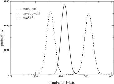
Figure 4: The probability distribution of 1-bits per individual, with ($p=0.5$) and without parasex ($p=0$), for mutation rates $m=3$ and $m=513$ (in this last case, at right, the curves for $p=0$ and $p=0.5$ coincide).

First, we studied this distribution when there is no parasex. We observed that for a very high mutation rate ($m\geq 512$), that is, if during the reproduction step half or more of the offspring genome is mutated, there is no selection effect: Genomes end up, on average, with half of the bits equal to one (maximum entropy). In this case the introduction of parasex has no visible effect and the probability distribution of 1-bits per individual seems to be a Gaussian centered at 512, in both cases (rightmost curve of Fig.4.).

For small mutation rates, selection effects are already present even without parasex: The probability distribution is now centered at a value smaller than 512. The introduction of parasex moves the distribution towards an even smaller average number of 1-bits, as shown in Fig.4.

In order to confirm that these distributions are Gaussians, that is:

$$y=A\exp\biggl{[}{-\frac{(N-\langle N\rangle)^{2}}{2{\alpha}^{2}}}\biggr{]}$$

where $\langle N\rangle$ is the average number of 1-bits and $\alpha$ is the distribution width, we plot $Y=-\ln y$ as a function of $X=(N-\langle N\rangle)^{2}$, to check if we obtain straight lines for both sides of the distribution. The slope of these lines is proportional to $1/{\alpha^{2}}$. The results are shown in Fig.5, for a mutation rate of $m=513$.

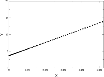
Figure 5: Linearization (see text) of the distributions with $m=513$ shown in Fig.4.

In this case where, as mentioned before, selection does not work, it can be seen that the distributions are indeed Gaussians.

However, from Fig.6 we can see that for small mutation rates ($m=3$) the tails of the distributions deviate from the Gaussian form, mainly when there is no parasex (circles). It occurs because selection is working and there are more individuals populating the left side of the distributions, than the right one. The reason why this deviation is stronger when there is no crossing is that parasex tends to mix the very clean genomes already selected by the dynamic process. However, this effect should not be confounded with a possible loss of diversity. On the contrary, besides improving the average genetic fitness of the whole population by pushing the distribution to the left, as shown in Fig.4, parasex in fact increases the diversity, i.e. the width of the distribution. Note the lower slope of the lines in Fig.6 when there is parasex. The role of the crossing mechanism is simply to offer a larger number of options to the Darwinian selection process.

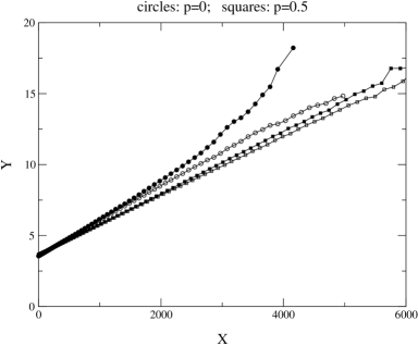
Figure 6: Linearization (see text) of the distributions with $m=3$, shown in Fig.4. The upper line corresponds to the right part of the distribution and the lower line to the left part. Circles: no parasex; Squares: parasex for $p=0.5$.

Similar results were obtained for smaller values of the parasex probability $p$. Also, in all cases the final steady state distribution of 1-bits is reached much faster when parasex is allowed. This is another advantage in what concerns the ability of the population to adapt to sudden environment changes.

3.3 Results for pure bad mutations

When only deleterious mutations are considered, without parasex all genomes end up with only 1-bits, independently of the value of the mutation rate. For real genomes this would result in a genetic population meltdown with the death of all individuals. The introduction of parasex is able to avoid this extinction, even for small probabilities of exchanging genomes. Fig.7. shows the probability distribution for genome lengths of 512 bits. Without parasex the distribution evolves to a delta-function at 512.

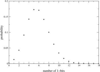
Figure 7: The probability distribution of 1-bits per individual, with parasex and only bad mutations. Parameters: $p=0.3$, $m=1$ and $P_{0}=1000$.

4 Conclusions

We have used three different models to simulate genome exchange between individuals, a possible intermediate behaviour between asexual and sexual reproduction. In all of them the genome of each individual is represented by one bit-string (haploid) and its fitness is related to the number of 1-bits accumulated in its genome. Every individual has a probability to exchange part of its genome with another individual randomly chosen among the same population, a process called parasex. We have observed that this exchanging of genomes always increase the survival chances, measured through the population size or through the probability distribution of 1-bits per genome, depending on the model. Even in extreme cases where the population evolves to genetic meltdown, the introduction of parasex is enough to avoid it.

Acknowledgements: To PMMH at ESPCI for the warm hospitality, to Sorin Tănase-Nicola for helping us with the computer facilities and to S. Cebrat for discussions; SMO and PMCO thank the Brazilian agency FAPERJ for financial support.

References

- [1] J.S. Sa Martins: Phys. Rev. E 61, 2212 (2000); R.S. Howard and C.M. Lively, Nature 367, 554 and 368, 358 (E) (1994).
- [2] R.J. Redfield: Nature 369, 145 (1994).
- [3] B. Örçal, E. Tüzel, V. Sevim, N. Jan and A. Erzan: Int. J. Mod. Phys. C 11, 973 (2000).
- [4] N. Jan, L. Moseley and D. Stauffer: Theory in Bioscience 119, 166 (2000).
- [5] T.J.P. Penna: J. Stat. Phys. 78, 1629 (1995).
- [6] S. Moss de Oliveira, P.M.C. de Oliveira, D. Stauffer: Evolution, Money, War and Computers, Teubner, Stuttgart and Leipzig 1999.
- [7] D. Stauffer, page 258 in: Biological Evolution and Statistical Physics, ed. by M. Lässig and A. Valleriani, Springer, Berlin Heidelberg 2002.
- [8] D. Stauffer, P.M.C. de Oliveira, S. Moss de Oliveira, T.J.P. Penna, J.S. Sa Martins: An. Acad. Bras. Ci. 73, 15 (2001) (condmat/0011524).
- [9] D. Stauffer, J.S. Sa Martins, S. Moss de Oliveira: Int. J. Mod. Phys. C 11, 1305 (2000); J.S. Sa Martins, D. Stauffer: Physica A, 294, 191 (2001).
- [10] P.M.C. de Oliveira: Theory Bioscience 120, 1 (2001) (condmat/0101170).
- [11] P.M.C. de Oliveira, S. Moss de Oliveira and Jan P. Radomski: Theory in Bioscience, 120, 77 (2001).
- [12] A. Ticona and P.M.C. de Oliveira: Int. J. Mod. Phys. C 12, 1075 (2001).
- [13] Jan P. Radomski and S. Moss de Oliveira: Int. J. Mod. Phys. C 11, 1297 (2000).