Spin-Orbit Coupling, Antilocalization, and Parallel Magnetic Fields in Quantum Dots

Abstract

We investigate antilocalization due to spin-orbit coupling in ballistic GaAs quantum dots. Antilocalization that is prominent in large dots is suppressed in small dots, as anticipated theoretically. Parallel magnetic fields suppress both antilocalization and also, at larger fields, weak localization, consistent with random matrix theory results once orbital coupling of the parallel field is included. In situ control of spin-orbit coupling in dots is demonstrated as a gate-controlled crossover from weak localization to antilocalization.

The combination of quantum coherence and electron spin rotation in mesoscopic systems produces a number of interesting and novel transport properties. Numerous proposals for potentially revolutionary electronic devices that use spin-orbit (SO) coupling have appeared in recent years, including gate-controlled spin rotators DattaDas as well as sources and detectors of spin-polarized currents SOPol . It has been predicted that the effects of some types of SO coupling will be strongly suppressed in small 0D systems, i.e., quantum dots Khaetskii ; Halperin ; RMT . This suppression as well as overall control of SO coupling will be important if quantum dots are used to store electron spin states as part of a future information processing scheme.

In this Letter, we investigate SO effects in ballistic-chaotic GaAs/AlGaAs quantum dots. We identify the signature of SO coupling in ballistic quantum dots to be antilocalization (AL), leading to characteristic magnetoconductance curves, analogous to known cases of disordered 1D and 2D systems HLK ; BergmannReview ; DresselhausExp ; Millo ; Miller ; Knap . AL is found to be prominent in large dots and suppressed in smaller dots, as anticipated theoretically Khaetskii ; Halperin ; RMT . Results are generally in excellent agreement with a new random matrix theory (RMT) that includes SO and Zeeman coupling RMT . Moderate magnetic fields applied in the plane of the 2D electron gas (2DEG) in which the dots are formed cause a crossover from AL to weak localization (WL). This can be understood as a result of Zeeman splitting, consistent with RMT RMT . At larger parallel fields WL is also suppressed, which is not expected within RMT. The suppression of WL is explained quantitatively by orbital coupling of the parallel field, which breaks time-reversal symmetry Falko . Finally, we demonstrate in situ electrostatic control of the SO coupling strength by tuning from AL to WL in a dot with a center gate.

It is well known that in mesoscopic samples coherent backscattering of time-reversed electron trajectories leads to a conductance minimum (WL) at $B=0$ in the spin-invariant case, and a conductance maximum (AL) in the case of strong SO coupling HLK . In semiconductor heterostructures, SO coupling results mainly from electric fields DyakanovPerel (appearing as magnetic fields in the electron frame) leading to momentum dependent spin precessions due to crystal inversion asymmetry (Dresselhaus term Dresselhaus ) and heterointerface asymmetry (Rashba term Rashba ).

SO coupling effects have been previously measured using AL in GaAs 2DEGs DresselhausExp ; Millo ; Miller and other 2D heterostructures Knap . Other means of measuring SO coupling in heterostructures, such as from Shubnikov-de Haas oscillations SdH and Raman scattering spectroscopy Jusserand are also quite developed. SO effects have also been reported in mesoscopic systems (comparable in size to the phase coherence length) such as Aharonov-Bohm rings, wires, and carbon nanotubes rwt . Recently, parallel field effects of SO coupling in quantum dots were measured Hackens ; Folk . In particular, an observed reduction of conductance fluctuations in a parallel field Folk was explained by including SO effects Halperin ; RMT , leading to an important extension of random matrix theory (RMT) to include new symmetry classes associated with SO and Zeeman coupling RMT .

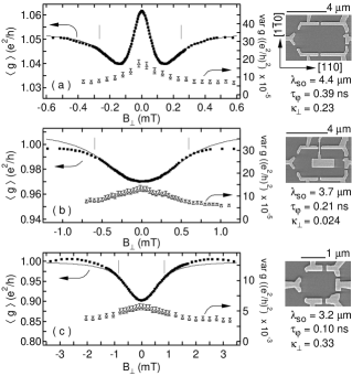
Figure 1: Average conductance $\langle g\rangle$ (squares) and variance of conductance $\mathrm{var}(g)$ (triangles) calculated from $\sim 200$ statistically independent samples (see text) as a function of perpendicular magnetic field $B_{\bot}$ for (a) $8.0\,\mathrm{\mu m^{2}}$ dot (b) $5.8\,\mathrm{\mu m^{2}}$ center-gated dot and (c) $1.2\,\mathrm{\mu m^{2}}$ dot at $T=0.3\,\mathrm{K}$, along with fits to RMT (solid curves). In (b), the center gate is fully depleted. Vertical lines indicate the fitting range, error bars of $\langle g\rangle$ are about the size of the squares.

This RMT addresses quantum dots coupled to two reservoirs via $N$ total conducting channels, with $N\gg 1$. It assumes $(\gamma,\epsilon_{Z})\ll E_{T}$, where $\gamma=N\Delta/(2\pi)$ is the level broadening due to escape, $\Delta$ is the mean level spacing, $\epsilon_{Z}=g\mu_{B}B$ is the Zeeman energy and $E_{T}$ is the Thouless energy (Table I). Decoherence is included as a fictitious voltage probe BBB ; RMT with dimensionless dephasing rate $N_{\varphi}=h/(\Delta\tau_{\varphi})$, where $\tau_{\varphi}$ is the phase coherence time. SO lengths $\lambda_{1,2}$ along respective principal axes $[110]$ and $[1\bar{1}0]$ are assumed (within the RMT) to be large compared to the dot dimensions $L_{1,2}$ along these axes. We define the mean SO length $\lambda_{so}=\sqrt{|\lambda_{1}\lambda_{2}|}$ and SO anisotropy $\nu_{so}=\sqrt{|\lambda_{1}/\lambda_{2}|}$. SO coupling introduces two energy scales: $\epsilon_{\bot}^{so}=\kappa_{\bot}E_{T}(L_{1}L_{2}/\lambda_{so}^{2})^{2}$, which represents a spin-dependent Aharonov-Bohm-like effect, and $\epsilon_{\parallel}^{so}\sim((L_{1}/\lambda_{1})^{2}+(L_{2}/\lambda_{2})^{2})\epsilon_{\bot}^{so}$, providing spin flips. AL appears in the regime of strong SO coupling, $(\epsilon_{\bot}^{so},\epsilon_{\parallel}^{so})\gg\tilde{\gamma}$, where $\tilde{\gamma}$ is the total level broadening $\tilde{\gamma}=(\gamma+\hbar/\tau_{\varphi})$. Note that large dots reach the strong SO regime more readily (i.e., for weaker SO coupling) than small dots. Parameters $\lambda_{so}$, $\tau_{\varphi}$, and $\kappa_{\bot}$ (a dimensionless parameter characterizing trajectory areas within the dot) are extracted from fits to dot conductance as a function of perpendicular field, $B_{\perp}$. The asymmetry parameter, $\nu_{so}$, is estimated from the dependence of magnetoconductance on parallel field, $B_{\parallel}$.

The quantum dots are formed by lateral Cr-Au depletion gates defined by electron-beam lithography on the surface of a GaAs/AlGaAs heterostructure grown in the [001] direction. The 2DEG interface is $349\,\mathrm{\AA}$ below the wafer surface, comprising a $50\,\mathrm{\AA}$ GaAs cap layer and a $299\,\mathrm{\AA}$ AlGaAs layer with two Si $\mathrm{\delta}$-doping layers $143\,\mathrm{\AA}$ and $161\,\mathrm{\AA}$ from the 2DEG. An electron density of $n\sim 5.8\times 10^{15}\,\mathrm{m^{-2}}$ Subb and bulk mobility $\mu\sim 24\,\mathrm{m^{2}/Vs}$ (cooled in the dark) gives a transport mean free path $\ell_{e}\sim 3\,\mathrm{\mu m}$. This 2DEG is known to show AL in 2D Miller . Measurements were made in a ³He cryostat at $0.3\,\mathrm{K}$ using current bias of $1\,\mathrm{nA}$ at $338\,\mathrm{Hz}$. Shape-distorting gates were used to obtain ensembles of statistically independent conductance measurements Chan95 while the point contacts were actively held at one fully transmitting mode each ($N=2$).

A	$\Delta$	$\tau_{d}$	$E_{T}/\Delta$	$\epsilon_{\bot}^{so}/\Delta$	$\epsilon_{\parallel}^{so}/\Delta$	$a_{1}$, $a_{2}$	$b_{2}$
$\,\mathrm{\mu m^{2}}$	$\mathrm{\mu eV}$	ns				$\mathrm{(ns)^{-1}T^{-2}}$	$\mathrm{(ns)^{-1}T^{-6}}$
1.2	6.0	0.35	33	0.15	0.04	6.6, 6.6	0.24
5.8	1.2	1.7	73	0.32	0.33	3.2, 0	140
8	0.9	2.3	86	3.6	3.1	1.4, 0.9	3.7

Table 1: Dot area $A=L_{1}L_{2}$ ($130\,\mathrm{nm}$ edge depletion); spin-degenerate mean level spacing $\Delta=2\pi\hbar^{2}/m^{*}A$ ($m^{*}=0.067m_{e}$); dwell time $\tau_{d}=h/(N\Delta)$; Thouless energy $E_{T}=\hbar v_{F}/\sqrt{A}$; $\epsilon_{\bot}^{so}/\Delta$ and $\epsilon_{\parallel}^{so}/\Delta$ for the fits in Fig. 1; $B^{2}$ coefficients $a_{1}$ and $a_{2}$ from one and two parameter fits; $B^{6}$ coefficient $b_{2}$ from two parameter fit, see text.

Figure 1 shows average conductance $\langle g\rangle$, and variance of conductance fluctuations, $\mathrm{var}(g)$, as a function of $B_{\perp}$ for the three measured dots: a large dot ($A\sim 8\,\mathrm{\mu m^{2}}$), a variable size dot with an internal gate ($A\sim 5.8\,\mathrm{\mu m^{2}}$ or $8\,\mathrm{\mu m^{2}}$, depending on center gate voltage), and a smaller dot ($1.2\,\mathrm{\mu m^{2}}$). Each data point represents $\sim 200$ independent device shapes. The large dot shows AL while the small and gated dots show WL. Estimates for $\lambda_{so}$, $\tau_{\varphi}$ and $\kappa_{\bot}$, from RMT fits are listed for each device below the micrographs in Fig. 1 (see Table I for corresponding $\epsilon_{\bot}$ and $\epsilon_{\parallel}$). When AL is present (i.e., for the large dot), estimates for $\lambda_{so}$ have small uncertainties ($\pm 5\%$) and give upper and lower bounds; when AL is absent (i.e., for the small and gated dots) only a lower bound for $\lambda_{so}$ ($-5\%$) can be extracted from fits. The value $\lambda_{so}\sim 4.4\,\mathrm{\mu m}$ is consistent with all dots and in good agreement with AL measurements made on an unpatterned 2DEG sample from the same wafer Miller .

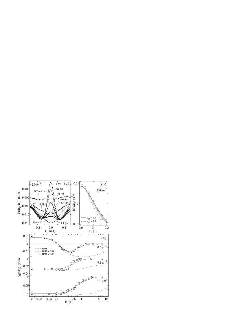
Figure 2: (a) Difference of average conductance from its value at large $B_{\bot}$, $\delta g(B_{\bot},B_{\parallel})$, as a function of $B_{\bot}$ for several $B_{\parallel}$ for the $8.0\,\mathrm{\mu m^{2}}$ dot at $T=0.3\,\mathrm{K}$ (squares) with RMT fits (curves). (b) Sensitivity of $\delta g(0,B_{\parallel})$ to $\nu_{so}$ for the $8.0\,\mathrm{\mu m^{2}}$ dot, $1\leq\nu_{so}\leq 2$ (shaded), $\nu_{so}=1.4$ (solid line) and $\nu_{so}=0.8$ (dashed line) (c) $\delta g(0,B_{\parallel})$ (markers) with RMT predictions (dashed curves) and one parameter (solid curves) or two parameter fits (dotted curves) using RMT including a suppression factor due to orbital coupling of $B_{\parallel}$, see text.

Comparing Figs. 1(a) and 1(c), and recalling that all dots are fabricated on the same wafer, one sees that AL is suppressed in smaller dots, even though $\lambda_{so}$ is sufficient to produce AL in the larger dot. We note that these dots do not strongly satisfy the inequalities $L/\lambda_{so}\ll 1,N\gg 1$, having $N=2$ and $L/\lambda_{so}=0.64\ (0.34)$ for the large (small) dot. Nevertheless, Fig. 1 shows the very good agreement between experiment and the new RMT.

We next consider the influence of a parallel magnetic field on average magnetoconductance. In order to apply tesla-scale $B_{\parallel}$ while maintaining subgauss control of $B_{\perp}$, we mount the sample with the 2DEG aligned to the axis of the primary solenoid (accurate to $\sim 1^{\circ}$) and use an independent split-coil magnet attached to the cryostat to provide $B_{\perp}$ as well as to compensate for sample misalignment Folk . Figure 2 shows plots of the deviation of the shape-averaged conductance from its value at $B_{\perp}\gg\phi_{0}/A$ (i.e., with time-reversal symmetry fully broken by $B_{\perp}$), $\delta g(B_{\bot},B_{\parallel})=\langle g(B_{\bot},B_{\parallel})\rangle-\langle g(B_{\perp}\gg\phi_{0}/A,B_{\parallel})\rangle$. Figure 2(a) shows $\delta g(B_{\bot},B_{\parallel})$ as a function of $B_{\bot}$ at several values of $B_{\parallel}$, along with fits of RMT RMT in which parameters $\lambda_{so}$, $\tau_{\varphi}$ and $\kappa_{\bot}$ have been set by a single fit to the $B_{\parallel}=0$ data. The low-field dependence of $\delta g(0,B_{\parallel})$ on $B_{\parallel}$ (Fig. 2(b)) then allows the remaining parameter, $\nu_{so}$, to be estimated as described below.

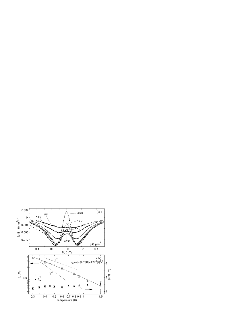
Figure 3: (a) Difference of average conductance from its value at large $B_{\bot}$, $\delta g(B_{\bot},0)$, for various temperatures with $B_{\parallel}=0$ for the $8.0\,\mathrm{\mu m^{2}}$ dot (squares), along with RMT fits (solid curves). (b) Spin-orbit lengths $\lambda_{so}$ (circles) and phase coherence times $\tau_{\varphi}$ (triangles) as a function of temperature, from data in (a).

Besides $\epsilon_{Z}$ (which is calculated using $g=-0.44$ rather than fit), parallel field combined with SO coupling introduces an additional new energy scale, $\epsilon^{Z}_{\perp}={\kappa_{z}\epsilon_{Z}^{2}A\over 2E_{T}}\sum_{i,j=1,2}{l_{i}\over\lambda_{i}}{l_{j}\over\lambda_{j}}$, where $\kappa_{Z}$ is a dot-dependent constant and $l_{1,2}$ are the components of a unit vector along $B_{\parallel}$ RMT . Because orbital effects of $B_{\parallel}$ on $\delta g(B_{\perp},B_{\parallel})$ dominate at large $B_{\parallel}$, $\epsilon^{Z}_{\perp}$ must instead be estimated from RMT fits of $\mathrm{var}(g)$ with already-broken time reversal symmetry, which is unaffected by orbital coupling Zumbuhlvar .

The RMT formulation RMT is invariant under $\nu_{so}\rightarrow r/\nu_{so}$, where $r=L_{1}/L_{2}$ sym , and gives an extremal value of $\delta g(0,B_{\parallel})$ at $\nu_{so}=\sqrt{r}$. As a consequence, fits to $\delta g(0,B_{\parallel})$ cannot distinguish between $\nu_{so}$ and $r/\nu_{so}$. As shown in Fig. 2(b), data for the $8\mathrm{\mu m^{2}}$ dot ($r\sim 2$) are consistent with $1\leq\nu_{so}\leq 2$ and appear best fit to the extremal value, $\nu_{so}\sim 1.4$. Values of $\nu_{so}$ that differ from one indicate that both Rashba and Dresselhaus terms are significant, which is consistent with 2D data taken on the same material Miller .

Using $\nu_{so}=1.4$ and values of $\lambda_{so}$, $\tau_{\varphi}$, and $\kappa_{\bot}$ from the $B_{\parallel}=0$ fit, RMT predictions for $\delta g(B_{\bot},B_{\parallel})$ agree well with experiment up to about $B_{\parallel}\sim\,0.2\,\mathrm{T}$ (Fig. 2(a)), showing a crossover from AL to WL. For higher parallel fields, however, experimental $\delta g$’s are suppressed relative to RMT predictions. By $B_{\parallel}\sim 2\,\mathrm{T}$, WL has vanished in all dots (Fig. 2(c)) while RMT predicts significant remaining WL at large $B_{\parallel}$. The full range of $\delta g(0,B_{\parallel})$ for the three dots is shown in Fig. 2(c). The center-gated ($5.6\,\mathrm{\mu m^{2}}$) dot and the small ($1.2\,\mathrm{\mu m^{2}}$) dot show WL for all $B_{\parallel}$, and a similar suppression of WL above $B_{\parallel}\sim 2\,\mathrm{T}$.

One would expect WL/AL to vanish once orbital effects of $B_{\parallel}$ break time reversal symmetry. Following Ref. Falko (FJ), we account for this with a suppression factor $f_{FJ}(B_{\parallel})=(1+\tau_{B\parallel}^{-1}/\tau_{esc}^{-1})^{-1}$, where $\tau_{B\parallel}^{-1}\sim aB_{\parallel}^{2}+bB_{\parallel}^{6}$, and assume that the combined effects of SO coupling and flux threading by $B_{\parallel}$ can be written as a product, $\delta g(0,B_{\parallel})=\delta g_{RMT}(0,B_{\parallel})\cdot f_{FJ}(B_{\parallel})$. The $B_{\parallel}^{2}$ term reflects surface roughness or dopant inhomogeneities; the $B_{\parallel}^{6}$ term reflects the asymmetry of the quantum well. We consider fits taking $a$ as a fit parameter ($a_{1}$, Table I) with $b=1.4\,10^{8}\,\mathrm{s^{-1}T^{-6}}$ fixed, obtained from self-consistent simulations FJsim , or allowing both $a$ and $b$ to be fit parameters ($a_{2}$ and $b_{2}$, Table I). Figure 2(c) shows that allowing both to be free is only significant for the (unusually shaped) center-gated dot; for the small and large dots, the single-parameter ($a$) fit gives good quantitative agreement.

We next consider the effects of temperature and dephasing. We find that increased temperature reduces the overall magnitude of $\delta g$ and also suppresses AL compared to WL, causing AL at $300\,\mathrm{mK}$ to become WL by $1.5\,\mathrm{K}$ (maximum of $\delta g(B_{\bot},0)$ at $B_{\bot}=0$ becomes minimum) in the $8\,\mathrm{\mu m^{2}}$ dot (Fig. 3a). Fits of RMT to $\delta g(B_{\perp},0)$ yield $\lambda_{so}$ values that are roughly independent of temperature (Fig. 3b), consistent with 2D results Millo , and $\tau_{\varphi}$ values that decrease with increasing temperature. Dephasing is well described by the empirical form $(\tau_{\varphi}\mathrm{[ns]})^{-1}\sim 7.5\,\mathrm{T[K]}+2.5\,\mathrm{(T[K])^{2}}$, consistent with previous measurements in low-SO dots HuibersDephasing . As temperature increases, long trajectories that allow large amounts of spin rotations are being cut off by the decreasing $\tau_{\varphi}$ and the AL peak is diminished, as observed.

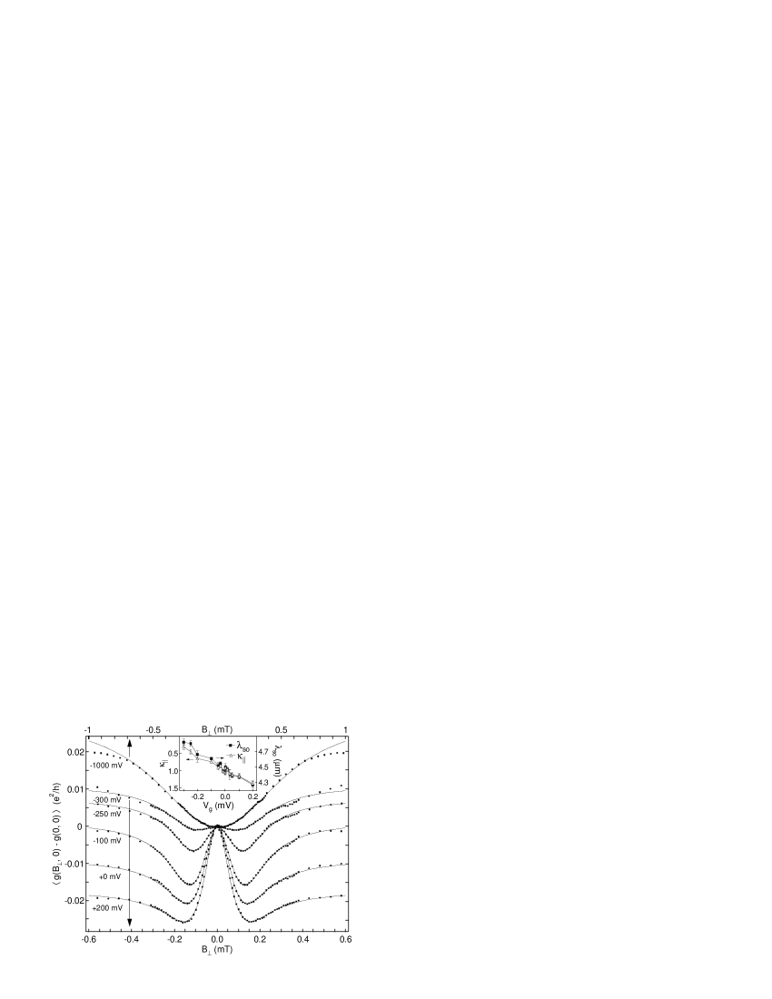
Figure 4: Difference of average conductance $\langle g\rangle$ from its value at $B_{\bot}=0$ as a function of $B_{\bot}$ for various center gate voltages $V_{g}$ in the center-gated dot (squares), along with fits to RMT RMT . Good fits are obtained though the theory assumes homogeneous SO coupling. Error bars are the size of the squares. Inset: $\lambda_{so}$ and $\kappa_{\parallel}$ as a function of $V_{g}$ extracted from RMT fits, see text.

Finally, we demonstrate in situ control of the SO coupling using a center-gated dot. Figure 4 shows the observed crossover from AL to WL as the gate voltage $V_{g}$ is tuned from $+0.2\,\mathrm{V}$ to $-1\,\mathrm{V}$. At $V_{g}=-1\,\mathrm{V}$, electrons beneath the center gate are fully depleted producing a dot of area $5.8\,\mathrm{\mu m^{2}}$ which shows WL. In the range of $V_{g}\geq-0.3$ V, the region under the gate is not fully depleted and the amount of AL is controlled by modifying the density under the gate. Note that for $V_{g}>0\,\mathrm{V}$ the AL peak is larger than in the ungated $8\,\mathrm{\mu m^{2}}$ dot. We interpret this enhancement not as a removal of the SO suppression due to an inhomogeneous SO coupling BrouwerInho , which would enhance AL in dots with $L/\lambda_{so}\ll 1$ (not the case for the $8\,\mathrm{\mu m^{2}}$ dot), but rather as the result of increased SO coupling in the higher-density region under the gate when $V_{g}>0\,\mathrm{V}$.

One may wish to use the evolution of WL/AL as a function of $V_{g}$ to extract SO parameters for the region under the gate. To do so, the dependence may be ascribed to either a gate-dependent $\lambda_{so}$ or to a gate-dependence of a new parameter $\kappa_{\parallel}=\epsilon_{\parallel}^{so}/(((L_{1}/\lambda_{1})^{2}+(L_{2}/\lambda_{2})^{2})\epsilon_{\bot}^{so})$. Both options give equally good agreement with the data (fits in Fig. 4 assume $\lambda_{so}(V_{g})$), including the parallel field dependence (not shown). Resulting values for $\lambda_{so}$ or $\kappa_{\parallel}$ (assuming the other fixed) are shown in the inset in Fig. 4. We note that the 2D samples from the same wafer did not show gate-voltage dependent SO parameters Miller . However, in the 2D case a cubic Dresselhaus term that is not included in the RMT of Ref. RMT was significant. For this reason, fits using RMT might show $\lambda_{so}(V_{g})$ though the 2D case did not. Further investigation of the gate dependence of SO coupling in dots will be the subject of future work.

We thank I. Aleiner, B. Altshuler, P. Brouwer, J. Cremers, V. Falko, J. Folk, B. Halperin, T. Jungwirth and Y. Lyanda-Geller. This work was supported in part by DARPA-QuIST, DARPA-SpinS, ARO-MURI and NSF-NSEC. Work at UCSB was supported by QUEST, an NSF Science and Technology Center. JBM acknowledges partial support from NDSEG.

References

- (1)
- (2) S. Datta and B. Das, Appl. Phys. Lett. 56, 665 (1990).
- (3) E. N. Bulgakov et al., Phys. Rev. Lett. 83, 376 (1999); A. A. Kiselev and K. W. Kim, Appl. Phys. Lett. 78, 775 (2001); S. Keppeler and R. Winkler, Phys. Rev. Lett. 88, 46401 (2002).
- (4) A. V. Khaetskii and Y. V. Nazarov, Phys. Rev. B 61, 12639 (2000); A. V. Khaetskii and Y. V. Nazarov, Phys. Rev. B 64, 125316 (2001).
- (5) B. I. Halperin et al., Phys. Rev. Lett. 86, 2106 (2001).
- (6) I. L. Aleiner and V. I. Fal’ko, Phys. Rev. Lett. 87, 256801 (2001); J. N. H. J. Cremers, P. W. Brouwer, B. I. Halperin, I. L. Aleiner and V. I. Fal’ko, (to be published).
- (7) S. Hikami et al., Prog. Theor. Phys. 63, 707 (1980); B. L. Al’tshuler et al., Sov. Phys. JETP 54, 411 (1981).
- (8) G. Bergmann, Phys. Rep. 107, 1 (1984).
- (9) P. D. Dresselhaus et al., Phys. Rev. Lett. 68, 106 (1992).
- (10) O. Millo et al., Phys. Rev. Lett. 65, 1494 (1990).
- (11) J. B. Miller, D. M. Zumbühl, C. M. Marcus, Y. B. Lyanda-Geller, K. Campman, and A. C. Gossard, cond-mat/0206375.
- (12) W. Knap et al., Phys. Rev. B 53, 3912 (1996).
- (13) V. I. Fal’ko and T. Jungwirth, Phys. Rev. B 65, 81306 (2002); J. S. Meyer et al., cond-mat/0105623 (2001).
- (14) M. I. D’yakanov and V. I. Perel’, Sov. Phys. JETP 33, 1053 (1971).
- (15) G. Dresselhaus, Phys. Rev. 100, 580 (1955).
- (16) Y. L. Bychkov, E. I. Rashba, J. Phys. C 17, 6093 (1983).
- (17) J. P. Heida et al., Phys. Rev. B 57, 11911 (1988); S. J. Papadakis et al., Science 283, 2056 (1999); D. Grundler, Phys. Rev. Lett. 84, 6074 (2000).
- (18) B. Jusserand et al., Phys. Rev. B 51, 4707 (1995).
- (19) Ç. Kurdak et al., Phys. Rev. B 46, 6846 (1992); A. G. Aronov and Y.B. Lyanda-Geller, Phys. Rev. Lett. 70, 343 (1993); A. F. Morpurgo et al., Phys. Rev. Lett. 80, 1050 (1998); J. Nitta et al., App. Phys. Lett. 75, 695 (1999); H. R. Shea et al., Phys. Rev. Lett. 84, 4441 (2000); H. A. Engel and D. Loss, Phys. Rev. B 62, 10238 (2000); A. Braggio et al., Phys. Rev. Lett. 87, 146802 (2001); F. Mireles and G. Kirczenow, Phys. Rev. B 64, 24426 (2001).
- (20) B. Hackens et al., Physica E 12, 833 (2002).
- (21) J. A. Folk et al., Phys. Rev. Lett. 86, 2102 (2001).
- (22) M. Büttiker, Phys. Rev. B 33, 3020 (1986); H. U. Baranger and P. A. Mello, Phys. Rev. B 51, 4703 (1995); P. W. Brouwer and C. W. J. Beenakker, Phys. Rev. B 55, 4695 (1997).
- (23) All measured densities are below the threshold for second subband occupation , which is known from Shubnikov-de Haas measurements and a decreasing mobility with increasing density near the threshold.
- (24) I. H. Chan et al., Phys. Rev. Lett. 74, 3876 (1995).
- (25) D. M. Zumbühl et at., (to be published).
- (26) The symmetry is precise if one takes . See Ref. RMT .
- (27) V. Falko, T. Jungwirth, private communication.
- (28) A. G. Huibers et al., Phys. Rev. Lett. 81, 200 (1998); A. G. Huibers et al., Phys. Rev. Lett. 83, 5090 (1999).
- (29) P. W. Brouwer et al., Phys. Rev. B 65, 81302 (2002).