Short-range interactions in a two-electron system: energy levels and magnetic properties

Abstract

The problem of two electrons in a square billiard interacting via a finite-range repulsive Yukawa potential and subjected to a constant magnetic field is considered. We compute the energy spectrum for both singlet and triplet states, and for all symmetry classes, as a function of the strength and range of the interaction and of the magnetic field. We show that the short-range nature of the potential suppresses the formation of “Wigner molecule” states for the ground state, even in the strong interaction limit. The magnetic susceptibility $\chi(B)$ shows low-temperature paramagnetic peaks due to exchange induced singlet-triplet oscillations. The position, number and intensity of these peaks depend on the range and strength of the interaction. The contribution of the interaction to the susceptibility displays paramagnetic and diamagnetic phases as a function of $T$.

I Introduction

The study of mesoscopic systems has proved to be a rich field to investigate explicit manifestations of quantum properties in nanometer and micron scales Mesosc_review . In such systems, the electron coherence length scales and mean-free paths are in general larger than the typical sample sizes, so that the underlying classical electronic motion plays an important role. The nature of the classical motion, regular, mixed or chaotic, reflects itself on some of the quantum properties of the system, particularly in the energy level distribution. These features have long been studied for non-interacting chaos_nonint and weakly interacting systems harold .

In quantum dots, where few electrons are laterally confined kastner , the electron-electron interaction is usually very efficiently shielded by the positively charged fixed ions and other effects, so that the independent electron gas theory can often be used to understand the basic features of the system ullmo ; report ; levy ; prado1 ; prado ; agam ; oppen . However, the residual interaction that survives the shielding can sometimes play important roles. In recent years, much attention has been given to interaction-induced effects in mesoscopic systems bedanov ; peeters ; harold ; creffield1 ; creffield2 ; grigorenko ; akbar . These effects are particularly important in the large-dot regime, where the electron-electron Coulomb interaction overcomes the kinetic energy, forcing the ground-state into a Wigner molecule type of configuration creffield1 .

In mesoscopic systems the electronic interaction is usually not well approximated by a bare long-range Coulomb force, due exactly to screening effects ando . The strength and range of the residual interaction, or the efficiency of the screening, depend on many parameters, like the electron density and size of the dot. It is therefore important to understand the effects of the interaction as a function of its effective intensity and range. In this work we give a contribution in this direction presenting exact results for the problem of two electrons in a square quantum dot interacting via a repulsive finite-range Yukawa type of interaction, $V(r)=V_{0}e^{-\alpha r}/r$, and subjected to a uniform and constant magnetic field of strength $B$ applied perpendicular to the dot. This model system was inspired by the experimental work of Levy et al levy where the orbital magnetic susceptibility was measured for an ensemble of square dots containing of the order of a thousand electrons each. Although the independent particle semiclassical theory explained most of the experimental findings ullmo ; report ; levy ; prado1 ; prado ; agam ; oppen , the behavior of the susceptibility with the temperature does not come out correctly in this approach and still puzzles the theorists. The idea that the slow decay of the susceptibility observed experimentally (as opposed to the exponential decay expected from the semiclassical theory), could be due to electron-electron interaction was first investigated in harold for a weak contact (Dirac delta) type of interaction using perturbation methods. In this article we study the effects of electronic interaction a much simpler system, with only two electrons, but we present exact (numerical) results.

The choice of an Yukawa type of potential allows us to interpolate between the pure Coulomb ($\alpha=0$) and short range interactions. Besides, the calculation of the Hamiltonian matrix elements can be reduced to one-dimensional integrals, which can be calculated numerically. This allows us to compute the energy spectrum for the four rotational symmetry classes as a function of the interaction strength $V_{0}$ and range $1/\alpha$ for both singlet and triplet states. We also consider these results as a function of a constant magnetic field of strength $B$ applied perpendicular to the square. We compute the magnetic susceptibility at finite values of the magnetic field and temperature via the partition function.

Our main results can be summarized as follows: (1) $V_{0}$ introduces avoided crossings between the energy levels within each symmetry class, one of the signatures of quantum chaos; (2) $\alpha$ has a very important role in determining the probability profile of the ground state, suppressing in some cases the Wigner molecule type of behavior even for strong interactions; (3) The effect of the interaction on the magnetic susceptibility $\chi(B)$ depends on $\alpha$. In particular, for large magnetic fields, singlet-triplet oscillations of the ground state level lead to paramagnetic fluctuations on the two-electron susceptibility $\chi(B)$, in contrast to the non-interacting diamagnetic susceptibility. The position and intensity of these peaks change with the range of the interaction.; (4) The contribution to the susceptibility induced by interaction at zero magnetic field shows paramagnetic and diamagnetic phases as a function of the temperature. This type of behavior has also been found for weak Dirac delta interactions harold .

This paper is organized as follows: in section II we describe the system in detail. We discuss its symmetry properties and compute the matrix elements of the Hamiltonian. In section III we present numerical results for the energy spectrum and for ground-state electronic density as a function of the strength and range of the interaction. In section IV we consider the magnetic properties of the system and in section V we discuss our results.

II Hamiltonian and Matrix Elements

We consider a system where two electrons are confined in a square-shaped two dimensional billiard of size $L$ interacting via an Yukawa type of potential and subjected to a uniform and constant magnetic field of strength $B$ applied perpendicular to the dot. The Hamiltonian is given by

$$H= \frac{1}{2m^{*}}\sum_{i=1,2}(p_{xi}+eBy_{i}/2)^{2}+(p_{yi}-eBx_{i}/2)^{2})$$ (1)

$$+V_{walls}+V_{0}\frac{e^{-\alpha|\vec{r}_{1}-\vec{r}_{2}|}}{|\vec{r}_{1}-\vec{r}_{2}|}$$

where $m^{*}$ is the quasiparticle electron mass and $V_{walls}$ is the square well potential. The eigenfunctions of a single particle in this square dot with zero magnetic field are given by a normalized product of sine functions:

$$\varphi_{mn}(x,y)=\left(\frac{2}{L}\right)\sin{\frac{m\pi}{L}x}\sin{\frac{n\pi}{L}y}$$ (2)

and the eigenenergies are simply

$$E_{mn}=\frac{\hbar^{2}}{2m^{*}L^{2}}\pi^{2}(m^{2}+n^{2})$$ (3)

The square billiard is a highly symmetric system. It is invariant under the action of 8 symmetry operations (4 rotations plus 4 reflections) which form the ${\mathcal{C}}_{4v}$ symmetry group. When the time-reversal symmetry is broken (e.g. by the application of a magnetic field), the Hamiltonian is no longer invariant under reflections. The group then reduces to ${\mathcal{C}}_{4}$, formed by the four rotations generated by $\hat{C}_{4}$ (rotation by $\frac{\pi}{2}$ ). The symmetric eigenfunctions can be written as a linear combination of a particular eigenfunction and its symmetry-related counterparts:

$$\psi(x,y)=\varphi(x,y)+\hat{C_{4}}\varphi(x,y)+\hat{C^{2}_{4}}\varphi(x,y)+\hat{C^{3}_{4}}\varphi(x,y)\;.$$ (4)

Rotating $\psi$ leads to $\hat{C_{4}}\psi=e^{i\theta}\psi$ with $(e^{i\theta})^{4}=1$. This, in turn, leads to four solutions for $e^{i\theta}$, namely $+1,-1,+i$ and $-i$. We can thus separate the general eigenfunctions (2) in four “classes” (or representations) using the group’s character table hammermesh , as follows:

$$\begin{array}[]{rcl}\psi_{mn}^{(+1)}(x,y)&=&\left\{\begin{array}[]{lll}\varphi_{mn}(x,y)&&\mbox{\small if $n=m$ (both odd)}\\ \lx@intercol\frac{1}{\sqrt{2}}\left(\varphi_{mn}(x,y)(\pm)\varphi_{nm}(x,y)\right)\hfil\lx@intercol\\ &&\mbox{\small if $n\neq m$ and both odd (even)}\end{array}\right.\\[2.84544pt] \psi_{mn}^{(-1)}(x,y)&=&\left\{\begin{array}[]{lll}\varphi_{mn}(x,y)&&\mbox{\small if $n=m$ (both even)}\\ \lx@intercol\frac{1}{\sqrt{2}}\left(\varphi_{mn}(x,y)(\mp)\varphi_{nm}(x,y)\right)\hfil\lx@intercol\\ &&\mbox{\small if $n\neq m$ and both odd (even)}\end{array}\right.\\[2.84544pt] \psi_{mn}^{(+i)}(x,y)&=&\left\{\begin{array}[]{lll}\frac{1}{\sqrt{2}}\left(\varphi_{mn}(x,y)\right.&\pm&i\varphi_{nm}(x,y))\\ &\lx@intercol\mbox{\small if $m$ even (odd) $n$ odd (even)}\hfil\lx@intercol\end{array}\right.\\[2.84544pt] \psi_{mn}^{(-i)}(x,y)&=&\left\{\begin{array}[]{lll}\frac{1}{\sqrt{2}}\left(\varphi_{mn}(x,y)\right.&\mp&i\varphi_{nm}(x,y))\\ &\lx@intercol\mbox{\small if $m$ even (odd) $n$ odd (even)}\hfil\lx@intercol\end{array}\right.\\[2.84544pt] \end{array}$$ (5)

This equation can be written in a more compact form as

$$\psi^{(C)}_{l}=F^{(C)}_{l}\left(\varphi_{l}+S^{(C)}_{l}\varphi_{\bar{l}}\right)$$ (6)

where $l\equiv(m,n)$ and $\bar{l}\equiv(n,m)$. $F^{(C)}_{l}$ is either $1$ or $\frac{1}{\sqrt{2}}$ and $S^{(C)}_{l}$ is $0$, $\pm 1$ or $\pm i$, depending on the symmetry class $(C)$ and on $l$ (whether $(m,n)$ is odd/even and whether $m=n$ or $m\neq n$).

Finally the two-particle orbital eigenfunctions are symmetrized $(S)$ or anti-symmetrized $(A)$ combinations of one-particle orbital eigenfunctions:

$$\psi^{(S,A),(C_{1}\otimes C_{2})}_{l_{1}l_{2}}(\vec{r_{1}},\vec{r_{2}})=$$

$$\frac{1}{\sqrt{2}}\left(\psi_{l_{1}}^{(C_{1})}(\vec{r_{1}})\psi_{l_{2}}^{(C_{2})}(\vec{r_{2}})\pm\psi_{l_{1}}^{(C_{1})}(\vec{r_{2}})\psi_{l_{2}}^{(C_{2})}(\vec{r_{1}})\right)$$

The orbital eigenfunction is symmetrized if the electrons are in the singlet spin state and anti-symmetrized if they are in the triplet spin state.

The symmetry group of the two-particle system is ${\mathcal{C}}_{4}\otimes{\mathcal{C}}_{4}$ and the eigenfunctions still separate in four symmetry classes. The two-particle ($2p$) class is defined by the total phase gained under the action of an element of the ${\mathcal{C}}_{4}\otimes{\mathcal{C}}_{4}$ group ($E\otimes\hat{C}_{4}$, $\hat{C}_{4}\otimes\hat{C}_{4}$ and so on). This phase is simply the product of the one-particle ($1p$) phases in the representation shown in (5). The $2p$ class is thus obtained in a simple manner by “multiplying” the $1p$ classes. For instance, two $1p$ states of class $(-1)$ form a $2p$ state of class $(+1)$ [pictorically, $(+1)$ ”=” $(-1)\otimes(-1)$]. The same happens with a $1p$ state of class $(+i)$ combined with other from class $(-i)$. On the other hand, two $1p$ $(+i)$ states form a $(-1)$ $2p$ state and so on.

II.1 The screened Coulomb interaction

For the electron-electron interaction we have used an “Yukawa type” short-range screened Coulomb potential

$$V(\vec{r_{1}},\vec{r_{2}})=\frac{e^{2}}{4\pi\epsilon_{0}\epsilon_{r}}\frac{e^{-\alpha|\vec{r_{1}}-\vec{r_{2}}|}}{|\vec{r_{1}}-\vec{r_{2}}|}$$ (8)

where $1/\alpha$ is the interaction range and $\epsilon_{r}$ is the dielectric constant of the two-dimensional electron gas (in case of a GaAs 2DEG, $\epsilon_{r}=10.9$). The reason for this particular choice of screening is two-fold. First it interpolates between the pure Coulomb case and localized interactions. Also it gives an effective “interaction length” ($\alpha^{-1}$) which is easy to control. Second, the $1/r$ dependence is maintained with the screening appearing as an exponential (as opposed to a power of $1/r$). This facilitates enormously the calculation of the matrix elements, as we show in the appendix. The range $\alpha$ will be considered here as a free parameter.

The Hamiltonian for the two electrons without the magnetic field is given by

$$\hat{H}=\sum_{i=1}^{2}\left(\frac{1}{2m_{i}^{*}}\vec{p_{i}}^{2}\right)+V(\vec{r_{1}},\vec{r_{2}})\;.$$ (9)

Since the kinetic energy (3) scales with $1/L^{2}$ and the interaction scales with $1/L$, the electron-electron interaction term dominates over the kinetic term for large $L$. Thus, we define an “effective potential strength” $V_{0}$ that grows linearly with the dot size $L$:

$$V_{0}\equiv L\frac{e^{2}}{4\pi\epsilon_{0}\epsilon_{r}}\left(\frac{2m^{*}}{\hbar^{2}\pi^{2}}\right)$$ (10)

so that we can write the matrix elements of $\hat{H}$ in the non-interacting basis in units of $(\pi^{2}\hbar^{2})/(2m^{*}L^{2})$:

$$<\psi^{(C)}_{l_{1}l_{2}}|\hat{H}|\psi^{(C)}_{l_{1}l_{2}}>=\frac{\pi^{2}\hbar^{2}}{2m^{*}L^{2}}\left\{\bar{E}_{l_{1}l_{2}}+V_{0}<\psi^{(C)}_{l_{1}l_{2}}|\hat{V}(r/L)|\psi^{(C)}_{l_{1}l_{2}}>\right\}$$ (11)

where $\bar{E}_{l_{1}l_{2}}=(m_{1}^{2}+n_{1}^{2}+m_{2}^{2}+n_{2}^{2})$ is the kinetic energy in units of $(\pi^{2}\hbar^{2})/(2m^{*}L^{2})$. This defines another free parameter, $V_{0}$ (or, equivalently, $L$) that controls the relative interaction strength.

The next step is to calculate the matrix elements of the potential in the two-particle eigenfunction basis defined by Eq.(LABEL:psi2p). The repulsive potential does not break the ${\mathcal{C}}_{4}\otimes{\mathcal{C}}_{4}$ rotational symmetry of the Hamiltonian, since it depends only on the distance between the electrons. Therefore, the interaction matrix is block-diagonal in this representation, i.e. the matrix elements

$$V_{l_{1}l_{2}l^{{}^{\prime}}_{1}l^{{}^{\prime}}_{2}}=\left<\psi^{S,A,(\mbox{\scriptsize{Class}})}_{l_{1}l_{2}}|\hat{V}|\psi^{S,A,(\mbox{\scriptsize{Class}})}_{l^{{}^{\prime}}_{1}l^{{}^{\prime}}_{2}}\right>$$ (12)

are non-zero only inside the same symmetry block. For totally symmetric (antisymmetric) eigenfunctions $V_{l_{1}l_{2}l^{{}^{\prime}}_{1}l^{{}^{\prime}}_{2}}$ breaks into a sum (difference) of the a direct and an exchange term. The general expression for the $\hat{V}$ matriz elements is given in terms of the general one-particle states Eq.(6) as

$$\begin{array}[]{l}\begin{array}[]{rcl}<\psi_{1}^{A}\psi_{2}^{B}|\hat{V}|\psi_{1^{{}^{\prime}}}^{C}\psi_{2^{{}^{\prime}}}^{D}>&=&F^{(A)}_{1}F^{(B)}_{2}F^{(C)}_{3}F^{(D)}_{4}\times\\[14.22636pt] \end{array}\\ \begin{array}[]{l}\left((1+S^{(A)}_{1}S^{(B)}_{2}S^{(C)}_{1^{{}^{\prime}}}S^{(D)}_{2^{{}^{\prime}}})<l_{1}l_{2}|\hat{V}|l^{{}^{\prime}}_{1}l^{{}^{\prime}}_{2}>+(S^{(A)*}_{1}S^{(B)*}_{2}S^{(C)*}_{1^{{}^{\prime}}}+S^{(D)}_{2^{{}^{\prime}}})<l_{1}l_{2}|\hat{V}|l^{{}^{\prime}}_{1}\bar{l}^{{}^{\prime}}_{2}>\right.\\ +(S^{(A)*}_{1}S^{(B)*}_{2}S^{(D)*}_{2^{{}^{\prime}}}+S^{(C)}_{1^{{}^{\prime}}})<l_{1}l_{2}|\hat{V}|\bar{l}^{{}^{\prime}}_{1}l^{{}^{\prime}}_{2}>+(S^{(A)*}_{1}S^{(C)*}_{1^{{}^{\prime}}}S^{(D)*}_{2^{{}^{\prime}}}+S^{(B)}_{2})<l_{1}\bar{l}_{2}|\hat{V}|l^{{}^{\prime}}_{1}l^{{}^{\prime}}_{2}>\\ +(S^{(B)*}_{2}S^{(C)*}_{1^{{}^{\prime}}}S^{(D)*}_{2^{{}^{\prime}}}+S^{(A)}_{1})<\bar{l}_{1}l_{2}|\hat{V}|l^{{}^{\prime}}_{1}l^{{}^{\prime}}_{2}>+(S^{(A)*}_{1}S^{(B)*}_{2}+S^{(C)}_{1^{{}^{\prime}}}S^{(D)}_{2^{{}^{\prime}}})<l_{1}l_{2}|\hat{V}|\bar{l}^{{}^{\prime}}_{1}\bar{l}^{{}^{\prime}}_{2}>\\ \left.+(S^{(A)*}_{1}S^{(C)*}_{1^{{}^{\prime}}}+S^{(B)}_{2}S^{(D)}_{2^{{}^{\prime}}})<l_{1}\bar{l}_{2}|\hat{V}|l^{{}^{\prime}}_{1}\bar{l}^{{}^{\prime}}_{2}>+(S^{(B)*}_{2}S^{(C)*}_{1^{{}^{\prime}}}+S^{(A)}_{1}S^{(D)}_{2^{{}^{\prime}}})<\bar{l}_{1}l_{2}|\hat{V}|l^{{}^{\prime}}_{1}\bar{l}^{{}^{\prime}}_{2}>\right)\;.\\ \end{array}\\ \end{array}$$ (13)

The terms $<l_{1}l_{2}|\hat{V}|l^{{}^{\prime}}_{1}l^{{}^{\prime}}_{2}>$ can be written explicitly with help of Eq.(2) as

$$\left<l_{1}l_{2}|\hat{V}|l^{{}^{\prime}}_{1}l^{{}^{\prime}}_{2}\right>=\frac{16}{L^{4}}\int\sin{\frac{\pi m_{1}x_{1}}{L}}\sin{\frac{\pi n_{1}y_{1}}{L}}\sin{\frac{\pi m_{2}x_{2}}{L}}\sin{\frac{\pi n_{2}y_{2}}{L}}\;V(|\vec{r_{2}}-\vec{r_{1}}|)\;\sin{\frac{\pi m_{1}^{{}^{\prime}}x_{1}}{L}}\sin{\frac{\pi n_{1}^{{}^{\prime}}y_{1}}{L}}\sin{\frac{\pi m_{2}^{{}^{\prime}}x_{2}}{L}}\sin{\frac{\pi n_{2}^{{}^{\prime}}y_{2}}{L}}\;d^{2}\vec{r_{1}}d^{2}\vec{r_{2}}$$ (14)

Eq.(13) can be further simplified using the property $\left<l_{1}l_{2}\right|\hat{V}\left|l^{{}^{\prime}}_{1}l^{{}^{\prime}}_{2}\right>=\left<\bar{l}_{1}\bar{l}_{2}\right|\hat{V}\left|\bar{l}^{{}^{\prime}}_{1}\bar{l}^{{}^{\prime}}_{2}\right>$. The integrals in Eq.(14) can be evaluated by switching to relative polar $(r,\theta)$ and center-of-mass coordinates. Thanks to the exponential form of the screening, three of the four integrals in (14) can be done analytically. The remaining integral, over the relative polar angle $\theta$, is performed numerically. Most of the direct and exchange elements involve less than 16 integrals. The number is actually $\frac{16}{2^{N}}$ where $N$ is the number of one-particle states with $m=n$ involved in either one of the two-particle functions. All these facts reduce the number of numerical integrals to be evaluated. The details of this calculation are on Appendix A.

II.2 The magnetic field

For $B\neq 0$, there are additional terms in the kinetic matrix element of (1) proportional to $B$ and $B^{2}$. These terms lead to integrals combining sine and cosine functions and powers of $x$ and $y$, which can all be done analytically.

The terms linear in $B$ (involving $\hat{p}_{y}$ and $\hat{p}_{y}$) contribute imaginary parts to the matrix elements, breaking the degeneracy of the $(+i)$ and $(-i)$ symmetry classes. This is a consequence of the time-reversal symmetry breaking.

III Effects of interaction: strength and range

In this section, we show the numerical results obtained with the exact diagonalization of the two-particle interacting Hamiltonian without the magnetic field. We discuss the effects of the two independent parameters of our model: the strength $V_{0}$ and the range $\alpha$. To change the intensity of the interaction relative to the kinetic energy we need to change $L$ (see Eq.(10)). However, changing $L$ changes the energy levels even if $V_{0}=0$. Therefore, in order to focus on the changes induced only by the potential, we shall measure the energy in units of $\frac{\pi^{2}\hbar^{2}}{2m^{*}L^{2}}$ throughout this section. In these units, the non-interacting eigen-energies are independent of $L$; the ground state energy, in particular, is equal to 4.

III.1 Energy levels

We first consider the effects of the interaction strength $V_{0}$. To increase $V_{0}$ relative to the kinetic energy we need to increase $L$. That, however, decreases the effective range of the interaction. To keep the ratio between range and size of the dot fixed, and concentrate on the effects of the potential strength, we shall keep the relative range $1/(\alpha L)$ fixed as $L$ (or $V_{0}$) is changed. When $1/(\alpha L)>1$, the electrons “feel” the presence of each other all over the dot. For $1/(\alpha L)<1$, the interaction is more localized and the interaction range reduced.

Figure 1 shows the two-particle energy levels as a function of the interaction strength for different values of $\alpha L$. All energy levels are shown, for the four symmetry classes of both singlet and triplet configurations. The first panel shows the Coulomb case, $\alpha=0$. The interaction induces singlet-triplet gaps creffield2 and removes several degeneracies in the energy levels. It also promotes level repulsion (“avoided crossings”) within each symmetry class. These are typical of systems with GOE-type level spacing distribution. Although the number of levels does not allow for a precise statistical analysis of the spectrum, the level-spacing histograms (not shown) display a distinctive difference between the non-interacting (Poisson-like) and the interacting (GOE-like) cases. As the relative range decreases ($\alpha L$ increases) the levels become less sensitive to $V_{0}$ and the avoided crossings narrow.

III.2 Ground-state properties

Recent works have investigated the formation of “Wigner molecule” type of ground states in polygonal quantum-dots in the low density limit creffield1 ; grigorenko ; akbar . In this limit, the Coulomb interaction between the electrons dominates over the kinetic energy (the so called “large $r_{s}$” limit) and the ground state electron density shows pronounced peaks near the corners of the polygonal boundary creffield1 .

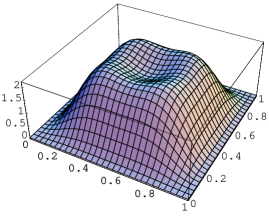
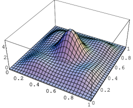
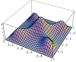
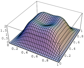
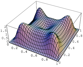
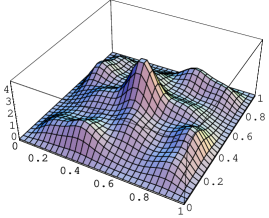
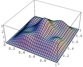
Figure 2: Electronic density for different values of $\alpha^{-1}$ and $L$. For each line, the reach parameter $\alpha^{-1}$ is fixed for increasing values of $L$ (from left to right $L=10,100$ and $1000$nm). From top to bottom, we have $\alpha^{-1}=10,100$ and $1000$nm. The Wigner Molecule state is recovered for $\alpha^{-1}=L=1\mu m$

We have addressed the question of whether the finite-range character of the repulsive potential would change such configuration. The low-density limit can be approached by making $V_{0}\rightarrow\infty$. However, as discussed above, as the dot size $L$ increases, the interaction strength increases but the effective interaction range $\alpha^{-1}$ decreases. Figure 2 shows that, depending on the value of $\alpha^{-1}$, the Wigner molecule state can be suppressed, even for large dots. This figure shows the ground-state electronic density

$$\rho(\vec{r_{1}})=\int|\Psi_{0}(\vec{r_{1}},\vec{r_{2}})|^{2}d\vec{r_{2}}$$ (15)

for $L=10$, $100$ and $1000$ $nm$ and $\alpha^{-1}=10$, $100$ and $1000$ $nm$. Each column represents dots with the same width $L$ but with different values of $\alpha$. Each line has the same value of $\alpha$ but different sizes. The product $\alpha L$ is constant along the diagonal. Even for the largest dot, with $1000nm$, the Wigner molecule state is completely suppressed for $\alpha L<10$ (first two plots on the last column). Only when $\alpha L=1$ (last plot on the last column) does the electron density show pronunced peaks near the corners.

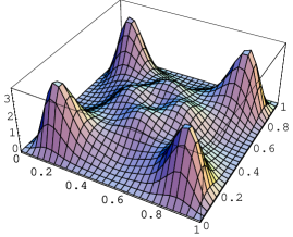
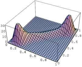
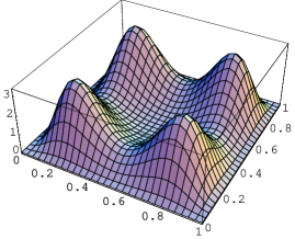
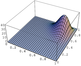
Figure 3: Top: Electronic density (right) and probability density with one of the coordinates on a Wigner molecule peak ($|\Psi^{(C)}_{0}({\bf r_{1}}=(0.2,0.2),{\bf r_{2}})|^{2}$) (middle) showing a singlet-like spatial correlation (right). Bottom: Same for an excited triplet state [(+i)-Class]

Figure 3 shows two examples of states with peaks near the corners in the strong interaction limit. We see that, although the electronic density of the two states looks similar, the spatial correlations are very different, reflecting the fact that one of them is a singlet and the other a triplet. Fixing ${\bf r}_{1}$ at the center of one of the peaks, $\bar{{\bf r}}_{1}=(0.2,0.2)$, the probability density $|\Psi({\bf r_{1}}=\bar{{\bf r}}_{1},{\bf r_{2}})|^{2}$ shows two peaks along the diagonal for the singlet state and only one peak on the opposite corner for the triplet state, since $\psi=0$ for ${\bf r}_{1}={\bf r}_{2}$ in this case. The two-particle configuration is shown schematically for both cases.

IV Effects of the interaction in the magnetic properties

IV.1 Energy levels

Figure 4 shows the first energy levels as a function of the magnetic field for $L=200$ nm and different values of $\alpha$. The first plot shows the non-interacting case ($V_{0}=0$), where the singlet and triplet two-particle levels are degenerate. Notice that the symmetry classes $(+i)$ and $(-i)$ are no longer degenerate for $B\neq 0$. Also, when the electronic interaction is switched on (Figs.4(b) and (c)), the singlet-triplet degeneracy is broken. The combination of these two effects leads to singlet-triplet crossings in the ground state for magnetic fields of the order of a few Tesla. This kind of oscillation has been studied previously both theoretically (for the Coulomb case) wagner ; peeters ; ugajin ; creffield2 and experimentally ashoori ; ashoori2 .

The role of the potential range $\alpha$ can also be seen from these figures. In Fig.4(b), where the range is only one tenth of the dot size, the splitting between the $(+i)$ and $(-i)$ classes is still very clear, but the scale of the energy levels is much closer to the non-interacting case. Also, and more importantly, there is only one singlet-triplet crossing in the ground state, as opposed to the three crossings of the Coulomb case. For smaller values of $\alpha^{-1}$ these crossings are completely suppressed.

IV.2 Partition function and susceptibility

In this subsection we consider the orbital magnetization and magnetic susceptibility of the interacting two-electron system. The partition function $Z(B,T)=\mathit{Tr}\{e^{-\beta\hat{H}(B)}\}$ ($\beta\equiv 1/k_{B}T$) can be computed from the energy levels. The magnetization $m(B)$ and the magnetic susceptibility $\chi(B)=\partial m(B)/\partial B$ can be calculated from

$$m(B)=-\frac{1}{A}\;\frac{\partial F}{\partial B}=\frac{1}{\beta A}\frac{\partial\log Z(B,T)}{\partial B}\;,$$ (16)

where $F$ is the Helmholtz free energy and $A=L^{2}$.

Figure 5 shows the magnetization $m(B,T)$, the susceptibility $\chi(B,T)$ and the interaction-induced susceptibility $\chi^{int}=\chi-\chi^{(0)}$ as a function of $B$ for $\alpha=0$ (Coulomb potential) and $\alpha^{-1}=L/10$ (short-range interaction). $\chi^{(0)}$ is the susceptibility of the non-interacting system. Both $\chi(B,T)$ and $\chi^{int}(B,T)$ are expressed in units of the Landau susceptibility $|\chi_{L}|=e^{2}/12\pi m^{*}c^{2}$ and the temperature is expressed in units of the mean level spacing $\Delta$.

On the average, $\chi(B,T)$ is diamagnetic, as in the non-interacting case (see $\chi^{(0)}$ on the inset). However, the exchange-induced singlet-triplet crossings of the ground state level contributes paramagnetic fluctuations of order of $\sim 3\chi_{L}$ at low temperatures. As discussed in the previous subsection, these crossings tend to disappear for short range interactions. For $\alpha L=10$ only one crossing survives.

For very low temperatures, only the ground state contributes significantly to the partition function and $F\approx E_{0}$. In the region close to the crossing, $\partial E_{0}/\partial B$ is discontinuous with a negative curvature, which explains the paramagnetic peak in $\chi(B)$. For higher temperatures, the “anti-crossing” (positive curvature) of the first excited state tends to compensate the ground state crossing and the fluctuations are attenuated.

Figure 6 shows the behavior of the interaction-induced susceptibility at zero magnetic field $\chi^{int}(B=0,T)$ for the Coulomb the and short-range ($\alpha^{-1}=L/10$) potentials and different values of the strength parameter $V_{0}$. The results show paramagnetic and diamagnetic phases as a $T$ increases, with a diamagnetic minimum at $T\approx 2\Delta$. For low values of $V_{0}$ the susceptibility is again paramagnetic for high $T$. This type of behavior has been observed before for weak contact (Dirac delta) type of interactions harold . Our results show that the existence of paramagnetic and diamagnetic phases in $\chi^{int}(B=0,T)$ might be more general, and not so sensitive to the type of interaction.

V Discussion

This work was motivated in part by the experimental results of Levy et al levy , who measured the magnetic properties of an ensemble of square dots containing a few thousands electrons each in the balistic regime. Our objective in this paper was to understand the effects of the residual electronic interaction in the simplest possible case, i.e., that of only two electrons. We simulated the shielding of the bare Coulomb force by using an exponential type of cut-off, like that of the Yukawa potential. The range of the interaction, $\alpha$, was considered as a free parameter. The size of the dot, which controls the relative strength of the potential, $V_{0},$ with respect to the kinetic energy, acts as a second parameter. Our results show that both $V_{0}$ and $\alpha$ are important to determine the properties of the energy spectrum and of the probability profile of the ground state. We showed, in particular, that short range interactions may suppress the appearance of Wigner molecule type of states even for strong interactions ($V_{0}$ large). The range of the interaction also affects the magnetic susceptibility of the system. Short range interactions might inhibit singlet-triplet oscillations of the ground state, suppressing the paramagnetic fluctuations of $\chi(B)$. Finally we have shown that the part of the susceptibility induced by the interaction presents paramagnetic and diamagnetic phases as a function of the temperature, in agreement with the results obtained by a pure Dirac delta interaction harold .

It is difficult speculate at this point if our results point to an explanation of the slow decay of the susceptibility with the temperature, as observed experimentally by Levy et al. In a system with many electrons, the ground state energy oscillates as a function of $B$ even without electronic interaction. This type of oscillation is only due to the boundary, and is responsible for the paramagnetic susceptibility of the gas. Our results indicate that, besides this “boundary-induced” effects, the electronic interaction is responsible for further oscillations, this time between singlet and triplet states. These “interaction-induced” oscillations also contribute to the susceptibility. In the present case of two electrons this contribution turns out to be larger than that of the non-interacting case. Besides, the curves in Fig. 6 show that $\chi^{int}(B=0,T)$ is sensitive to both $V_{0}$ and $\alpha$. The peak of $\chi^{int}(B=0,T)$ at $T\approx\Delta$ leads to a slightly slower decay of the overall susceptibility. Although this result might be peculiar of few-particle systems, there are similarities between our findings and those obtained from semiclassical analysis and RPA perturbation theory in the high-density limit harold , such as the diamagnetic minima in $\chi^{int}(B=0,T)$. This might indicate that the interaction indeed plays an important role in behavior of the susceptibility with the temperature, although calculations with more electrons should be conducted to confirm this conjecture.

Acknowledgements

This paper was partly supported by FAPESP, CNPq and Finep. LGGVDS would like to thank Prof. Harold U. Baranger for his contributions and support to the development of this work and acknowledges the hospitality of the Department of Physics at Duke University. We also would like to thank Dennis Ullmo, Gonzalo Usaj and Charles Creffield for helpful discussions and suggestions.

Appendix A Calculation of the integrals

In order to calculate the matrix element (14) we first notice that the integrand can be decoupled using relative and center-of-mass coordinates. Since the masses are equal (we set $m_{1}=m_{2}\equiv 1$ for simplicity), we have $\vec{r}=\vec{r_{2}}-\vec{r_{1}}$ and $\vec{R}=(\vec{R_{2}}+\vec{R_{1}})/2$. When the sine functions are written as a sum of complex exponentials

$$\begin{array}[]{rcl}\sin{2m\pi x_{i}}&=&\sum_{\epsilon_{i}=-1}^{1}\frac{\epsilon_{i}\;e^{\epsilon_{i}iM_{i}x_{i}}}{2i}\\[5.69046pt] \sin{2n\pi y_{i}}&=&\sum_{\eta_{i}=-1}^{1}\frac{\eta_{i}\;e^{\eta_{i}iN_{i}y_{i}}}{2i}\;,\end{array}$$

the integrand in Eq.(14) becomes

$$\sum_{\epsilon_{i}\eta_{i}}\frac{(\epsilon_{1}\cdots\epsilon_{2}^{{}^{\prime}})(\eta_{1}\cdots\eta_{2}^{{}^{\prime}})}{256}\times$$

$$\left(e^{i(\alpha_{1}+\alpha_{2})X}e^{i(\beta_{1}+\beta_{2})Y}e^{i(\alpha_{2}-\alpha_{1})\frac{x}{2}}e^{i(\beta_{2}-\beta_{1}){\frac{y}{2}}}\frac{e^{-\alpha r}}{r}\right)$$

where

$$\begin{array}[]{l}\alpha_{1}=\frac{\pi m_{1}}{L}\epsilon_{1}+\frac{\pi m_{1}^{{}^{\prime}}}{L}\epsilon_{1}^{{}^{\prime}}\;,\qquad\alpha_{2}=\frac{\pi m_{2}}{L}\epsilon_{2}+\frac{\pi m_{2}^{{}^{\prime}}}{L}\epsilon_{2}^{{}^{\prime}}\\ \beta_{1}=\frac{\pi n_{1}}{L}\eta_{1}+\frac{\pi n_{1}^{{}^{\prime}}}{L}\eta_{1}^{{}^{\prime}}\;,\qquad\beta_{2}=\frac{\pi n_{2}}{L}\eta_{1}+\frac{\pi n_{2}^{{}^{\prime}}}{L}\eta_{2}^{{}^{\prime}}\\ \end{array}$$ (18)

The integrals on the Center-of-Mass coordinates can then be readly evaluated, at the cost of working on the complex plane. However, one should note that the limits of integration of $(x,y)$ and $(X,Y)$ are not independent. In the rest of this development, we will take $L\equiv 1$ for the sake of simplicity. This is equivalent to perform the calculations on a adimensional variable $\frac{r}{L}$. In order to consider specific sizes for the dot, one has to include an additional factor of $L$ multiplying the whole integral and scale $\alpha$ accordingly.

The change of variables $(x_{1},y_{1},x_{2},y_{2})\rightarrow(x,y,X,Y)$ leads us to four different sets of integration limits (the quadrants on the $(x,y)$ plane). Next, we show the calculation of the integral on the first quadrant $(I_{1})$. The calculation on the other quadrants ($I_{2},I_{3},I_{4}$) is analogous. The total integral is then $I=I_{1}+I_{2}+I_{3}+I_{4}$. On the first quadrant we have

$$I_{1}=\sum_{\epsilon_{i}\eta_{i}}\frac{(\epsilon_{1}\cdots\epsilon_{2}^{{}^{\prime}})(\eta_{1}\cdots\eta_{2}^{{}^{\prime}})}{256}\times$$

$$\!\!\!\!\!\!\!\left(\int dA_{1}e^{i(\alpha_{1}+\alpha_{2})X}e^{i(\beta_{1}+\beta_{2})Y}e^{i(\alpha_{2}-\alpha_{1})\frac{x}{2}}e^{i(\beta_{2}-\beta_{1}){\frac{y}{2}}}\frac{e^{-\alpha\sqrt{x^{2}+y^{2}}}}{\sqrt{x^{2}+y^{2}}}\right)$$

where

$$\int dA_{1}=\int_{0}^{1}dx\int_{0}^{1}dy\int_{\frac{x}{2}}^{1-\frac{x}{2}}dX\int_{\frac{y}{2}}^{1-\frac{y}{2}}dY\,.$$ (20)

After doing the integrals on the center-of-mass coordinates we are left with

$$I_{1}=\sum_{\epsilon_{i}\eta_{i}}\frac{(\epsilon_{1}\cdots\epsilon_{2}^{{}^{\prime}})(\eta_{1}\cdots\eta_{2}^{{}^{\prime}})}{256}\left\{\int_{0}^{1}\int_{0}^{1}f(x,y)\frac{e^{-\alpha\sqrt{x^{2}+y^{2}}}}{\sqrt{x^{2}+y^{2}}}\;dxdy\right\}$$ (21)

where the exact format of $f(x,y)$ depends on whether we have $(\alpha_{1}+\alpha_{2})$ or $(\beta_{1}+\beta_{2})$ equal to zero or not. We are going to write it down explicitly in a moment.

A transformation to relative polar coordinates yields:

$$I_{1}=\sum_{\epsilon_{i}\eta_{i}}\frac{(\epsilon_{1}\cdots\epsilon_{2}^{{}^{\prime}})(\eta_{1}\cdots\eta_{2}^{{}^{\prime}})}{256}\left\{\int_{0}^{\frac{\pi}{2}}\int_{0}^{r_{1}(\theta)}f(r,\theta)e^{-\alpha r}\;drd\theta\right\}$$ (22)

where $r_{1}(\theta)=1/\cos{\theta}$ for $0<\theta<\frac{\pi}{4}$ and $r_{1}(\theta)=1/\sin{\theta}$ for $\frac{\pi}{4}<\theta<\frac{\pi}{2}$. The integral over $r$ can be done analytically and we are left with a set of integrals over $\theta$:

$$I_{1}=\sum_{\epsilon_{i}\eta_{i}}\frac{(\epsilon_{1}\cdots\epsilon_{2}^{{}^{\prime}})(\eta_{1}\cdots\eta_{2}^{{}^{\prime}})}{256}\left\{\int_{0}^{\frac{\pi}{2}}F(\theta)d\theta\right\}$$ (23)

As one can see from eq. (LABEL:Ik), the explicit form of $F(\theta)$ depends whether $(\alpha_{1}+\alpha_{2})$ and/or $(\beta_{1}+\beta_{2})$ are equal to zero or not. We now present the specific form of $F(\theta)$ for all different possibilities.

A.1 $(\alpha_{1}+\alpha_{2}),(\beta_{1}+\beta_{2})\neq 0$

$$F(\theta)=\frac{(-1)}{(\alpha_{1}+\alpha_{2})(\beta_{1}+\beta_{2})}\left[\frac{e^{(\alpha_{1}+\alpha_{2}+\beta_{1}+\beta_{2})}\left(e^{Z_{a}r_{1}}-1\right)}{Z_{a}(\theta)}+\frac{\left(e^{Z_{b}r_{1}}-1\right)}{Z_{b}(\theta)}+\frac{e^{(\alpha_{1}+\alpha_{2})}\left(1-e^{Z_{c}r_{1}}\right)}{Z_{c}(\theta)}+\frac{e^{(\beta_{1}+\beta_{2})}\left(1-e^{Z_{d}r_{1}}\right)}{Z_{d}(\theta)}\right]$$ (24)

A.2 $(\alpha_{1}+\alpha_{2})=(\beta_{1}+\beta_{2})=0$

$$F(\theta)=\frac{\left(e^{z_{a}r_{1}}-1\right)}{z_{a}(\theta)}-\frac{(\cos{\theta}+\sin{\theta})}{z_{a}^{2}(\theta)}\left[\left(e^{z_{a}r_{1}}(z_{a}r_{1}-1)+1\right)\right]+\frac{(\cos{\theta}\sin{\theta})}{z_{a}^{3}(\theta)}\left[\left(e^{z_{a}r_{1}}(z_{a}^{2}r^{2}_{1}-2z_{a}r_{1}+2)-2\right)\right]$$ (25)

A.3 $(\alpha_{1}+\alpha_{2})=0$ and $(\beta_{1}+\beta_{2})\neq 0$

$$F(\theta)=e^{(\beta_{1}+\beta_{2})}\frac{\left(e^{z_{b}r_{1}}-1\right)}{z_{b}(\theta)}-\frac{\left(e^{z_{c}r_{1}}-1\right)}{z_{c}(\theta)}-\cos{\theta}\left[e^{(\beta_{1}+\beta_{2})}\frac{\left(e^{z_{b}r_{1}}(z_{b}r_{1}-1)+1\right)}{z_{b}^{2}}-\frac{\left(e^{z_{c}r_{1}}(z_{c}r_{1}-1)+1\right)}{z_{c}^{2}}\right]$$ (26)

A.4 $(\alpha_{1}+\alpha_{2})\neq 0$ and $(\beta_{1}+\beta_{2})=0$

$$F(\theta)=e^{(\alpha_{1}+\alpha_{2})}\frac{\left(e^{z_{d}r_{1}}-1\right)}{z_{d}(\theta)}-\frac{\left(e^{z_{e}r_{1}}-1\right)}{z_{e}(\theta)}-\sin{\theta}\left[e^{(\alpha_{1}+\alpha_{2})}\frac{\left(e^{z_{d}r_{1}}(z_{d}r_{1}-1)+1\right)}{z_{d}^{2}}-\frac{\left(e^{z_{e}r_{1}}(z_{e}r_{1}-1)+1\right)}{z_{e}^{2}}\right]$$ (27)

where

$$\begin{array}[]{rcl}Z_{a}(\theta)&=&-\alpha-i\left(\alpha_{1}\cos{\theta}+\beta_{1}\sin{\theta}\right)\\ Z_{b}(\theta)&=&-\alpha+i\left(\alpha_{2}\cos{\theta}+\beta_{2}\sin{\theta}\right)\\ Z_{c}(\theta)&=&-\alpha-i\left(\alpha_{1}\cos{\theta}-\beta_{2}\sin{\theta}\right)\\ Z_{d}(\theta)&=&-\alpha+i\left(\alpha_{2}\cos{\theta}-\beta_{1}\sin{\theta}\right)\\ \\ z_{a}(\theta)&\equiv&-\alpha+i(\alpha_{2}\cos{\theta}+\beta_{2}\sin{\theta})\\ z_{b}(\theta)&\equiv&-\alpha+i(\alpha_{2}\cos{\theta}-\beta_{1}\sin{\theta})\\ z_{c}(\theta)&\equiv&-\alpha+i(\alpha_{2}\cos{\theta}+\beta_{2}\sin{\theta})\\ z_{d}(\theta)&\equiv&-\alpha+i(\beta_{2}\sin{\theta}-\alpha_{1}\cos{\theta})\\ z_{e}(\theta)&\equiv&-\alpha+i(\beta_{2}\sin{\theta}+\alpha_{2}\cos{\theta})\end{array}$$

All non-trivial integrals over $\theta$ have been performed numerically.

^∗ Present address: Universidade Federal de São Carlos, Dept. Física, 13565-905 São Carlos, SP, Brazil. Email: gregorio@df.ufscar.br

Figure 1: Energy levels as a function of $V_{0}$ for different values of the reach parameter $\alpha$. (a) $\alpha=0$ (Coulomb interaction), (b) $\alpha L=1$ and (d) $\alpha L=10$. Inset: avoided crossings on the $(+1)$-singlet (solid line) and $(-1)$-singlet (filled squares) classes

Figure 4: Energy levels as a function of $B$ for $L=200$nm and different values of the reach parameter $\alpha^{-1}$. (a) non-interacting ($V_{0}=0$), (b) $\alpha^{-1}=L/10$ and (c) Coulomb potential ($\alpha=0$)

Figure 5: Magnetization $m(B)$, magnetic susceptibility $\chi(B)$ and interaction induced susceptibility $\chi^{\mbox{\scriptsize int}}=\chi-\chi^{(0)}$ as a function on the magnetic field $B$ for a dot size of $L=200$nm and different values of the potential reach parameter $\alpha$ (Top: $\alpha=0$ [Coulomb], Bottom: $\alpha^{-1}=20$nm). For low temperatures $(T<\Delta/2)$, the system features interaction-induced paramagnetic peaks. Inset: The non-interacting magnetization and susceptibility.

Figure 6: Interaction-induced zero field susceptibility $\chi^{\mbox{\scriptsize int}}_{B=0}(T)$ as a function of the temperature for a Coulomb potential (left) and a Yukawa potential with $\alpha^{-1}=L/10$ (dir.) and different values of the potential strength $V_{0}$.

References

(1)Mesoscopic Quantum Physics, edited by
E. Akkermans, G. Montambaux, J.-L. Pichard, and J. Zinn-Justin
(Elsevier, New York, 1995).
(2)Quantum Chaos - Between order and disorder,
edited by G. Casati and B. Chirikov (Cambridge Univesity Press, New
York, 1995)
(3) D. Ullmo, H. Baranger, K. Richter, Felix von Oppen
and R. Jalabert, Phy. Rev. Lett. 80, 895 (1998)
(4) M.A. Kastner, Rev. Mod. Phys. 64, 849 (1992)
(5) D. Ullmo, K. Richter and R. Jalabert,
Phys. Rev. Lett. 74, 383 (1995)
(6) K. Richter, D. Ullmo and R. Jalabert
Phys. Rep. 276, 1 (1996)
(7) L.P. Lévy, D.H. Reich, L. Pfeiffer and
K. West, Physica B 189, 204 (1993)
(8) S.D. Prado and M.A.M. de Aguiar Phys. Rev.
E 54, 1369 (1996)
(9) S.D. Prado,M.A.M. de Aguiar, J.P Keating
and R. Egydio de Carvalho, J. Phys. A 27, 6091 (1994)
(20) I. Grigorenko. M.E. Garcia PhysicaA 291 (2001) 439-448;
(21) S. Akbar, In-Ho Lee Phys. Rev. B, 63
(2001) 165301
(22) T. Ando, A. B. Fowler, F. Stern, Rev. Mod. Phys.54, 437 (1982)
(23) M. Hammermesh, Group Theory and its
Application to Physical problems, Dover, 1989