Winner-Relaxing Self-Organizing Maps


Jens Christian Claussen
claussen@theo-physik.uni-kiel.de
Institut für Theoretische Physik und Astrophysik, Leibnizstr. 15,
Christian-Albrechts-Universität zu Kiel, 24098 Kiel, Germany

A new family of self-organizing maps, the Winner-Relaxing Kohonen Algorithm, is introduced as a generalization of a variant given by Kohonen in 1991. The magnification behaviour is calculated analytically. For the original variant a magnification exponent of 4/7 is derived; the generalized version allows to steer the magnification in the wide range from exponent 1/2 to 1 in the one-dimensional case, thus provides optimal mapping in the sense of information theory. The Winner Relaxing Algorithm requires minimal extra computations per learning step and is conveniently easy to implement.

1 Introduction

The self-organizing map (SOM) algorithm (Kohonen 1982) served both as model for topology-preserving primary sensory processing in the cortex (Obermayer et al. 1992), and for technical applications (Ritter et al. 1992). Self-organizing feature maps map an input space, such as the retina or skin receptor fields, into a neural layer by feedforward structures with lateral inhibition. Defining properties are topology preservation, error tolerance, plasticity, and self-organized formation by a local process. Compared to other clustering algorithms and vector quantizers its apparent advantage for data visualization and exploration is its approximative topology preservation. In contrast to the Elastic Net (Durbin & Willshaw 1987) and the Linsker (1989) Algorithm, which are performing gradient descent in a certain energy landscape, the Kohonen algorithm lacks an energy function in the general case of a continuous input distribution. Although the learning process can be described in terms of a Fokker-Planck equation (Ritter & Schulten 1988), the expectation value of the learning step is a nonconservative force (Obermayer et al. 1992) driving the process so that it has no associated energy function. Despite a lot of research, the relationships between the Kohonen model and its variants to general principles remain an open field (Kohonen 1991).

To appear in Neural Computation

1.1 Kohonen’s Self Organizing Feature Map

Kohonen’s Self Organizing Map is defined as follows: Every stimulus ${\bf v}$ of an input space $V$ is mapped to a “center of excitation”, or winner

$$\mbox{${\bf s}$}=\mbox{$\mbox{\rm argmin}_{{\bf r}\in R}|{\bf w}_{{\bf r}}-{\bf v}|$},$$ (1)

where $|.|$ denotes the Euclidian distance in input space. In the Kohonen model, the learning rule for each synaptic weight vector ${\bf w}_{{\bf r}}$ is given by

$$\delta{\bf w}_{{\bf r}}=\eta\cdot g_{{\bf r}{\bf s}}\cdot({\bf v}-{\bf w}_{{\bf r}}),$$ (2)

where $g_{{\bf r}{\bf s}}$ defines the neighborhood relation in $R$, and will throughout this paper be a Gaussian function of the Euclidian distance $|{\bf r}-{\bf s}|$ in the neural layer. Topology preservation is enforced by the common update of all weight vectors whose neuron ${\bf r}$ is adjacent to the center of excitation ${\bf s}$; the adjacency function $g_{{\bf r}{\bf s}}$ prescribes the topology in the neural layer. The speed of learning $\eta$ usually is decreased during the process.

1.2 The Winner Relaxing Kohonen Algorithm

We now consider an energy function $V$ first proposed in (Ritter et al. 1992). If we have a discrete input space, the potential function for the expectation value of the learning step is given by

$$V(\{{\bf w}\})=\frac{1}{2}\sum_{{\bf r}{\bf s}}g^{\gamma}_{{\bf r}{\bf s}}\sum_{\mu|{\bf v}^{\mu}\in F_{{\bf s}}(\{{\bf w}\})}p({\bf v}^{\mu})\cdot|{\bf v}^{\mu}-{\bf w}_{{\bf r}}|^{2},$$ (3)

where $F_{{\bf s}}(\{{\bf w}\})$ is the cell of the Voronoi tesselation (or Dirichlet tesselation) of input space defined by (1). For discrete input space, where $p({\bf v})$ is a sum over delta peaks $\delta({\bf v}-{\bf v}^{\mu})$, the first derivative w.r.t. ${\bf w}_{{\bf r}}$ is not continuous at all weight vectors where the borders of the voronoi tesselation are shifting over one of the input vectors (Fig. 1).

Figure 1: Shift of Voronoi borders as an effect of weight vector update.

However, (3) requires the assumption that none of the borders of the Voronoi tesselation is shifting over a pattern vector ${\bf v}^{\mu}$, which may be fulfilled in the final convergence phase for discrete input spaces, but becomes problematic if there are more receptor positions than neurons. If $p({\bf v})$ is continuous, the sum over $\mu$ becomes an integral, and with every stimulus vector update the surrounding Voronoi borders slide over stimuli (which means they become represented by annother weight vector), so that there is no global energy function for the general case.

We remark that replacing the crisp (or hard) winner selection (1) by a soft-winner ${\bf s}=\mbox{argmin}_{\bf r}\sum_{{\bf r^{\prime}}}g_{{\bf rr^{\prime}}}|{\bf w}_{{\bf r^{\prime}}}-{\bf v}|^{2}$ minimizes (3) even in the continuous case (Graepel et al 1997, Heskes 1999). This is a formally elegant approach if one wants to ensure the existence of an energy function and accepts to modify the winner selection.

However, to motivate the Winner Relaxing learning, we return to the hard winner selection scheme (1) and take up the learning rule given by Kohonen (1991). Our use of this ansatz however is justified here only a posteriori by its use for adjusting the magnification.

From the shift of the borders of the Voronoi tesselation $F_{{\bf s}}(\{{\bf w}\})$ (see Fig. 1) in evaluation of the gradient with respect to a weight vector ${\bf w}_{{\bf r}}$, Kohonen (1991) derived for the (approximated) gradient descent in $V$ the additive term $-\frac{1}{2}\eta\delta_{{\bf r}{\bf s}}\sum_{{\bf r}^{{}^{\prime}}\neq{\bf s}}g_{{\bf r}^{{}^{\prime}}{\bf s}}({\bf v}-{\bf w}_{{\bf r}^{{}^{\prime}}})$ extending (2) for the winning neuron. As it implied an additional elastic relaxation, it was straightforward to call it ‘Winner Relaxing’ (WR) Kohonen algorithm (Claussen 1992). In the remainder we study the (generalized) Winner Relaxing Kohonen algorithm, or Winner Relaxing Self-Organizing Map (WRSOM), introduced firstly in (Claussen 1992), in the form

$$\delta{\bf w}_{{\bf r}} = \eta\{({\bf v}-{\bf w}_{{\bf r}})g^{\gamma}_{{\bf r}{\bf s}}-\lambda\delta_{{\bf r}{\bf s}}\sum_{{\bf r}^{{}^{\prime}}\neq{\bf s}}g^{\gamma}_{{\bf r}^{{}^{\prime}}{\bf s}}({\bf v}-{\bf w}_{{\bf r}^{{}^{\prime}}})\},$$ (4)

where ${\bf s}$ is the center of excitation for incoming stimulus ${\bf v}$, and $g^{\gamma}_{{\bf r}{\bf s}}$ is a Gaussian function of distance in the neural layer with characteristic length $\gamma$. Here $\lambda$ is a free parameter of the algorithm. The original algorithm (associated with the potential function) proposed by Kohonen in 1991 is obtained for $\lambda=+1/2$, whereas the classical Self Organizing Map Algorithm is obtained for $\lambda=0$. The influence of $\lambda$ on the magnification behaviour is the central issue of this paper.

1.3 The Magnification Factor

The magnification factor is defined as the density of neurons ${\bf r}$ (i.e. the density of synaptic weight vectors ${\bf w}_{{\bf r}}$) per unit volume of input space, and therefore is given by the inverse Jacobi determinant of the mapping from input space to neuron layer: $M=|J|^{-1}=|\det({{d}}{\bf w}/{{d}}{\bf r})|^{-1}$. We assume the input space to be continuous and of same dimension as the neural layer, and the map to be noninverting $(J>0)$.

The magnification factor quantifies the networks’ response to a given probability density of stimuli $P({\bf v})$. To evaluate $M$ in higher dimensions, one in general has to compute the equilibrium state of the whole network and needs therefore the complete global knowledge on $P({\bf v})$, except for separable cases. For one-dimensional mappings the magnification factor can follow an universal magnification law, that is, $M(\bar{{\bf w}}({\bf r}))$ is a function of the local probability density $P$ only, independent of both the location ${\bf r}$ in the neural layer and the location $\bar{{\bf w}}({\bf r})$ in input space. Hereby it is nontrivial whether there exists a power law or not; the Elastic Net obeys an universal magnification law that remarkably is not a power law (Claussen & Schuster 2002) due to a nonvanishing elastic tension in regions of small input density. For the classical Kohonen algorithm the magnification law is given by a power law $M(\bar{{\bf w}}({\bf r}))\propto P(\bar{{\bf w}}({\bf r}))^{\rho}$ with exponent $\rho=\frac{2}{3}$ (Ritter & Schulten 1986). See Table 1 for an overview. For a discrete neural layer and different neighborhood kernels corrections apply (Ritter 1991, Ritter et al. 1992, Dersch& Tavan 1995).

Elastic	VQ,	WRK	SOM	WRK	Linsker
Net	NG	$\lambda=\frac{1}{2}$	$\lambda=0$	$\lambda=-1$
$\displaystyle\frac{1}{1+\frac{\kappa}{\sigma^{2}}\frac{P}{J}}$	$P^{\displaystyle 1/3}$	$P^{\displaystyle 4/7}$	$P^{\displaystyle 2/3}$	$P^{\displaystyle 1}$	$P^{\displaystyle 1}$

Table 1: Magnification laws for one-dimensional maps

As the brain is assumed to be optimized by evolution for information processing, one could conjecture that maximal mutual information can define an extremal principle governing the setup of neural structures. For feedforward neural structures with lateral inhibition, an algorithm of maximal mutual information has been defined by Linsker (1989) using the gradient descend in mutual information. It requires computationally costly integrations, and has a highly nonlocal learning rule; therefore it is neither favourable as a model for biological maps, nor feasible for technical applications. Due to realization constraints, both technical applications and cortical networks (Plumbley 1999) are not necessarily capable of reaching this optimum. Even if one had experimental data of the magnification behaviour, the question from what self-organizing dynamics neural structures emerge, remains. Overall it is desirable to find learning rules that minimize mutual information in a simpler way.

An optimal map from the view of information theory would reproduce the input probability exactly ($M\sim P({\bf v})^{\rho}$ with $\rho=1$), being equivalent to the condition that all neurons in the layer are firing with same probability. This defines an equiprobabilistic mapping (van Hulle 2000). An exponent $\rho=0$, on the other hand, corresponds to a uniform distribution of weight vectors, or no adaptation at all. So the magnification exponent is a direct indicator, how far a Self Organizing Map algorithm is away from the optimum predicted by information theory.

2 Magnification Exponent of the Winner-Relaxing Kohonen Algorithm

We now derive the magnification law of the Winner-Relaxing Kohonen algorithm (4) for the case of a 1D$\to$1D map. Note that for higher dimensions analytical results can only be obtained for special degenerate cases of the input probability density and therefore lack generality.

The necessary condition for the final state of the algorithm is that the expectation value of the learning step vanishes for all neurons $r$:

$$\forall_{{r}{\in}R}\;\;\;\;0=\int{\rm d}{v}\;p({v})\delta\bar{w}_{{r}}({v}).$$ (5)

Since this expectation value is equal to the learning step of the pattern parallel rule, (5) is the stationary state condition for both serial and parallel updating, and also for batch updating. Thus we can proceed for these variants simultaneously (As synaptic plasticity is widely assumed to be based on integrative effects, one could claim that a parallel model is sufficient). The update rule (4) can be extended by an additional diagonal term controlled by $\mu$:

$$\delta{w}_{{r}} = \eta\{({v}-{w}_{{r}})\cdot g^{\gamma}_{{r}{s}}+\mu({v}-{w}_{{r}})\delta_{{r}{s}}$$ (6)

$$-\lambda\delta_{{r}{s}}\sum_{{r}^{{}^{\prime}}\neq{s}}g^{\gamma}_{{r}^{{}^{\prime}}{s}}({v}-{w}_{{r}^{{}^{\prime}}})\}.$$

By insertion of the update rule (6) one obtains

$$0 = \int{\rm d}s\;P(\bar{w}(s))J(s)g^{\gamma}_{rs}(\bar{w}(s)-\bar{w}(r))$$ (7)

$$+(\mu+\lambda)\cdot\underbrace{\int{\rm d}s\;P(\bar{w}(s))J(s)\delta_{rs}(\bar{w}(s)-\bar{w}(r))}_{\equiv 0}$$

$$\;\;-\lambda\cdot\int\int{\rm d}s\;{\rm d}r^{{}^{\prime}}\;P(\bar{w}(s))J(s)\delta_{rs}g^{\gamma}_{r^{{}^{\prime}}s}(\bar{w}(s)-\bar{w}(r^{{}^{\prime}}))$$

$$= \int{\rm d}s\;P(\bar{w}(s))J(s)g^{\gamma}_{rs}(\bar{w}(s)-\bar{w}(r))$$

$$\;\;+\lambda\cdot P(\bar{w}(r))J(r)\cdot\int{\rm d}r^{{}^{\prime}}\;g^{\gamma}_{r^{{}^{\prime}}r}(\bar{w}(r^{{}^{\prime}})-\bar{w}(r)).$$

The derivation can be performed analoguous to (Ritter, Martinetz & Schulten 1992). In the continuum limit there is always an exactly matching winning weight vector $\bar{w}_{s}=v$. Further the integration variable is substituted, ${\rm d}v={\rm d}\bar{w}_{s}=J(s){\rm d}s$, and we define the abbreviation $\bar{P}:=P(\bar{w}(r))$. In the first integrand $\bar{P}J$ has to be expanded in powers of $q:=s-r$. Within the second integral $\bar{P}J$ is evaluated only at $r$. Thus the integration yields in leading order in $q$:

$$0 = \gamma^{2}\left(\frac{{\rm d}\bar{w}}{{\rm d}r}\frac{{\rm d}(\bar{P}J)}{{\rm d}r}+\frac{1}{2}\bar{P}J\frac{{\rm d}^{2}\bar{w}}{{\rm d}r^{2}}\right)$$

$$+\lambda\cdot\bar{P}J\cdot\int{\rm d}q\;g^{\gamma}_{0q}\;(\!\!\!\!\!\underbrace{q\frac{{\rm d}\bar{w}}{{\rm d}r}}_{\mbox{\tiny contribution 0}}\!\!\!\!\!+\frac{q^{2}}{2}\frac{{\rm d}^{2}\bar{w}}{{\rm d}r^{2}})$$

$$0 = \gamma^{2}\left(J\frac{{\rm d}(\bar{P}J)}{{\rm d}r}+\frac{\bar{P}J}{2}\frac{{\rm d}J}{{\rm d}r}+\lambda\frac{\bar{P}J}{2}\frac{{\rm d}J}{{\rm d}r}\right).$$ (8)

Further we have to require $\gamma\neq 0,$ $P\neq 0,$ $d\bar{P}/dr\neq 0$. Then the ansatz of an universal local magnification law $J(r)=J(\bar{P}(r))$, i.e. $J$ depends only on the local value of $P$, that may be expected for the one-dimensional case only, requires $J$ to fulfill the differential equation

$$0 = \frac{J}{\bar{P}}+(1+\frac{1}{2}+\frac{\lambda}{2})\frac{{\rm d}J}{{\rm d}\bar{P}}$$ (9)

or

$$\frac{{\rm d}J}{{\rm d}\bar{P}} = -\frac{2}{3+\lambda}\frac{J}{\bar{P}}.$$ (10)

It has a power law solution, (provided that $\lambda\neq{-3}$), which verifies the ansatz made above, $J$ being a function of the local density only,

$$M=\frac{1}{J}\sim P(v)^{\mbox{${\frac{2}{3+\lambda}}$}}.$$ (11)

Thus the magnification exponent is given by $\frac{2}{3+\lambda}$ and can be tuned from $1/2$ to 1 (see Fig. 2) within the range of stability.

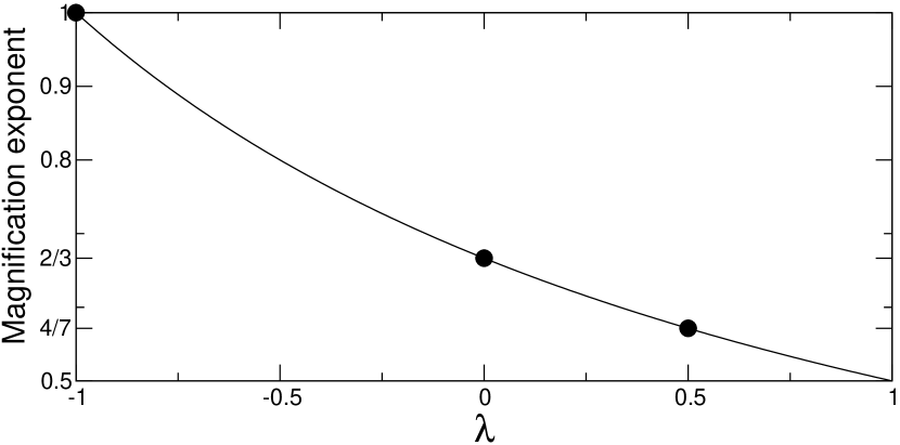
Figure 2: Impact of parameter $\lambda$ on the magnification exponent. The cases of $\lambda=1/2$ (Kohonen 1991), the SOM case $\lambda=0$ (Kohonen 1982) and the “winner enhancing” choice $\lambda=-1$ are marked with dots.

For the $\lambda=1/2$ choice of the Winner-Relaxing Kohonen Algorithm the magnification factor follows an exact power law with magnification exponent $\rho=4/7$, which is smaller than $\rho=2/3$ for the classical Self Organizing Feature Map (Ritter & Schulten 1986), but is still much larger than $\rho=1/3$ for Vector Quantization and Neural Gas. In any case, the maps resulting from the choices $\lambda=1/2$ and $\lambda=0$ are not optimal in terms of information theory.

3 Enhancing the Magnification

From this result one would try to invert the Relaxing Effect by choice of negative values for $\lambda$, which means to “enforce” the winner. In fact, the choice of $\lambda=-1$ leads to the magnification exponent 1.

The magnification law (11) is verified numerically as is shown in Table 2. Apart from the fact that the exponent can be varied by a priori parameter choice between $1/2$ and $1$, the simulations show that our Winner Relaxing Algorithm is able to establish information-theoretically optimal self-organizing maps in the “winner enforcing” case ($\lambda<0$).

$\!\!\downarrow\!\gamma$ $\lambda\!\rightarrow\!\!\!$	-1	-3/4	-1/2	-1/4	0	1/4	1/2	3/4	1
0.1	0.29	0.29	0.23	0.29	0.27	0.25	0.26	0.27	0.27
	$\pm$.04	$\pm$.04	$\pm$.04	$\pm$.04	$\pm$.05	$\pm$.04	$\pm$.04	$\pm$.04	$\pm$.05
0.5	0.49	0.46	0.43	0.45	0.43	0.40	0.39	0.37	0.34
	$\pm$.02	$\pm$.01	$\pm$.02	$\pm$.01	$\pm$.01	$\pm$.01	$\pm$.02	$\pm$.01	$\pm$.01
1.0	0.75	0.77	0.68	0.67	0.61	0.58	0.58	0.53	0.51
	$\pm$.04	$\pm$.02	$\pm$.02	$\pm$.02	$\pm$.01	$\pm$.01	$\pm$.01	$\pm$.01	$\pm$.01
2.0	0.93	0.86	0.77	0.71	0.65	0.61	0.57	0.53	0.50
	$\pm$.03	$\pm$.02	$\pm$.02	$\pm$.01	$\pm$.01	$\pm$.01	$\pm$.01	$\pm$.01	$\pm$.01
5.0	0.99	0.88	0.80	0.72	0.66	0.61	0.57	0.53	0.50
	$\pm$.05	$\pm$.04	$\pm$.03	$\pm$.02	$\pm$.02	$\pm$.02	$\pm$.02	$\pm$.02	$\pm$.02
Theory:	1.00	0.89	0.80	0.73	0.67	0.62	0.57	0.53	0.50

Table 2: Magnification exponent of the Winner Relaxing Algorithms determined numerically from a sample setup with $200$ neurons and $2\cdot{}10^{7}$ update steps and a learning rate of $0.1$. The input space was the unit interval, the stimulus probability density was chosen exponentially as $\exp(-\beta{}w)$ with $\beta=4$. After an adaptation period of $5\cdot{}10^{7}$ learning steps further $10\%$ of learning steps were used to calculate average slope and its fluctuation of $\log{}J$ as a function of $\log{}P.$ (The first and last $10\%$ of neurons were excluded to eliminate boundary effects). The small numbers denote the fluctuation of the exponent through the final $10\%$ of the experiment. For small $\gamma$, the neighborhood interaction becomes too weak. If the Gaussian neighborhood extends over some neurons ($\gamma=5$), the exponent follows the predicted dependence of $\gamma$ given by $2/(3+\lambda)$. For $|\lambda|>1$ the system is instable, this is the case where the additional update term of the winner is larger than the sum over all other update terms in the whole network. Tuning of the parameter $\mu$ did not seem to extend the region of stability. As the relaxing effect is inverted for $\lambda<0$, fluctuations are larger than in the Kohonen case.

4 Ordering time and Stability Region

At least for the 2D$\to$2D case, the Winner-Relaxing Kohonen Algorithm was reported as ‘somewhat faster’ (Kohonen 1991) in the initial ordering process. In a 1D$\to$1D sample setup (Claussen 2003), a marginally quicker ordering was observed for negative $\lambda$, at least at a relatively high learning rate $\eta=1$. As a lot of parameters and the input distribution itself influence the ordering time and decay of fluctuations, different results may be obtained; e.g., a small fraction of input distributions containing topological kinks take much longer to become ordererd, thus minimal, maximal, averaged, and inverse averaged ordering time will deviate.

If one instead investigates the time dependence of the fluctuations, for positive values of $\lambda$ a considerably quicker decay is observed (Fig. 4), being consistent with the observation by Kohonen (1991) mentioned above.

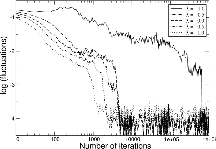
Figure 3: Time dependence (every tenth iterate shown) of the log rms fluctuations for different $\lambda$. Here the same setup of a single run with $\gamma=1.0$, $\eta=0.1$ and 10 neurons is being used; each run starts with the same configuration and random initial values between 0 and 1. For $\lambda>0$ a quicker ordering is observed.

Figure 4: Fast learning using a simple switching strategy. Starting with $\lambda=1/2$, ordering is acheived quickly. At iteration step 2000, $\lambda$ is immediately changed to -1 (dotted). This speeds up the learning phase by two orders of magnitude compared to starting with $\lambda=-1$, and by a factor 4 compared to $\lambda=0$ (dashed, shown for comparison). If the duration of the initial ordering phase is underestimated, again a long learning phase results (solid line; switch at step 200).

These simulations indicate that for obtaining optimal magnification, the price of a longer learning phase may have to be paid. However, this drawback can be circumvented by combining the advantages of both $\lambda$ ranges; i.e. using $\lambda>1$ in the initial phase to speed up ordering, and switching to $\lambda=-1$ after a considerable decay of fluctuations (Fig. 4). No complicated time-dependence of this parameter switch has been used, and neither learning rate nor neighborhood have been changed during the simulation.

The last important issue to be addressed is the dependence of stability on the parameter $\lambda$, especially at the border $-1$. Fortunately, the algorithm appears to be stable (in the 1D$\to$1D case) in the whole range $-1\leq\lambda\leq+1$, as shown in Fig. 5. On both borders the Winner Relaxing learning remains stable. Thus, the full range of magnification exponents between $1/2$ and $1$ can be acheived.

Figure 5: For $\mu\in[-1,+1]$ the common stability range is $\lambda\in[-1,+1]$. For $\lambda<-1$, the log rms of the weight vector differences $w_{r}-w_{r-1}$ diverges, but extremely long quiet transients are observed there. In the upper range $\lambda>+1$, making use of the diagonal term by using $\mu\neq{}0$ extends the stability range. The plots correspond to $10^{7}$ (straight), $10^{6}$ (dash-dotteded), and $10^{5}$ (dashed),respectively, for $\mu=0$. For $10^{7}$ iterations, also the cases $\mu=-1$ (thin dots) and $\mu=+1$ (thick dots) are shown. Parameters are $\gamma=1.0$, $\eta=0.1$, and 10 neurons are initialized near an equidistant chain with noise of amplitude 0.01 added.

In higher dimensions no universal magnification law is expected, but one can evaluate the output entropy for a given input distribution and network. As shown in Fig. 6, the enhancement of output entropy by Winner Relaxing learning is effective also in the twodimensional case, where however parameters have to be chosen more carefully.

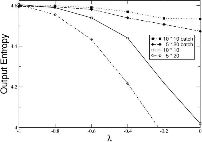
Figure 6: Entropy enhancement for the 2D$\to$2D case for network geometries of $10*10$ and $5*20$ neurons. The data density was $\sin({\pi}v_{1})\cdot\sin({\pi}v_{2})$ within the unit square, $\gamma=5.0$, and $\eta$ was decreased from $0.01$ to $0.001$ during $10^{6}$ learning steps. Alternatively, batch learning (over 100 steps) has been used; here $\eta$ was decreased from $0.05$ to $0.001$, $\gamma=2.0$ in the first $2\cdot 10^{5}$ steps ordinary SOM learning was applied ($\gamma=5.0$, $\lambda=0$). In all cases, for $\lambda=-1$ the entropy is enlarged compared to the unmodified case $\lambda=0$, and close to the optimum ($\ln 100=4.605$).

5 Discussion

After our first study (Claussen 1992), Herrmann et al. (1995) introduced annother modification of the learning process, which was also applied to the Neural Gas algorithm (Villmann & Herrmann 1998). Their central idea is to use a learning rate $\eta$ being locally dependent on the input probability density and also an exponent 1 can be obtained. As the input probability density should not be available to a neural map that self-organizes from stimuli drawn from that distribution, it is estimated from the actual local reconstruction mismatch (being an estimate for the size of the Voronoi cell) and from the time elapsed since the last time being the winner. Both operations require additional memory and computation, and, due to the estimating character, the learning rate has to be bounded in practical use. This localized learning was overall easier applicable and overcame the stability problems of the early approach of conscience learning (deSieno 1988).

Another systematic method, the extended Maximum Entropy Learning Rule, has been introduced by van Hulle (1997). It approximates a map of maximal output entropy for arbitrary dimension, alhough in higher dimensions the handling of the quantization regions becomes less practial (van Hulle 1998). A quite different approach being also capable of generating equiprobabilistic maps is via kernel optimization (van Hulle 1998, 2000, 2002), i.e.  neighborhood kernel radii themselves become learning parameters, in addition to the weight vectors defining the kernel centers. Other approaches, also influencing magnification, consider the selection of the winner to be probabilistic, leading to elegant statistical approaches to potential functions, as given by Graepel et al. (1997) and Heskes (1999).

As shown recently (Claussen & Villmann 2004), the Winner Relaxing concept can also be transferred successfully to the Neural Gas, confirming the utility of this class of learning rules.

6 Conclusions

The Linsker, Elastic Net and Winner-Relaxing Kohonen algorithms can be derived from an extremal principle, given by information theory, physical motivations, and reconstruction error, respectively. In this paper we have chosen the magnification law to indicate how close the algorithm reaches the adaptation properties of a map of maximal mutual information. The magnification law is one quantitative property that both is accessible by neurobiological experiments and manifests as a quantitative control parameter of a neural map used as vector quantizer in applications. A map of maximal mutual information uses all neurons with same probability, i.e. their firing rate will be equal.

In this work we have investigated the Winner Relaxing approach to establish a new family of vector quantizers. The shift from Kohonen ($\rho=2/3$) to Winner Relaxing Kohonen algorithm ($\rho=4/7$) seems to be marginal, if the emphasis is laid on the existence of a potential function. If a large magnification exponent is desired, the Winner Relaxing Kohonen Algorithm (with $\lambda=-1$) combines simple computation with a magnification corresponding to maximal mutual information.

Acknowledgements: The author wants to thank H.G. Schuster for raising attention to the topic and for stimulating discussions.

References

Claussen, J.C.  (born Gruel) (1992). Selbstorganisation Neuronaler Karten. Diploma thesis, Kiel, Germany.

Claussen, J.C.  & Schuster, H.G. (2002). Asymptotic level density of the Elastic Net Self-Organizing Map, Proc. ICANN 2002.

Claussen, J.C. (2003). Winner Relaxing and Winner-Enhancing Kohonen Maps: Maximal Mutual information from Enhancing the Winner. Complexity, 8(4), 15-22.

Claussen, J.C.  & Villmann, T. (2004). Magnification Control in Winner Relaxing Neural Gas. Neurocomputing, in print.

Dersch, D.R., & Tavan, P. (1995). Asymptotic level density in topological feature maps. IEEE Transactions on Neural Networks, 6, 230-236.

DeSieno, D. (1988). Adding a conscience to competitive learning. In: Proc. ICNN’88, International Conference on Neural Networks, pp. 117-124, IEEE Service Center, Piscataway, NJ.

Durbin, R. & Willshaw, D. (1987). An analogue approach to the Travelling Salesman Problem using an Elastic Net Method. Nature, 326, 689-691.

Herrmann, M., Bauer, H.-U., Der, R. (1995). Optimal Magnification Factors in Self-Organizing Maps. Proc. ICANN 1995, pp. 75-80.

Graepel, T., Burger, M., & Obermayer, K. (1997). Phase transitions in stochastic self-organizing maps. Phys. Rev. E, 56, 3876-3890.

Heskes, T. (1999). Energy functions for self-organizing maps. In: Oja and Karski, ed.: Kohonen Maps, Elsevier.

van Hulle, M. M. (1997). Nonparametric density estimation and regression achieved with topographic maps maximizing the information-theoretic entropy of their outputs. Biological Cybernetics, 77, 49-61.

van Hulle, M. M. (1998). Kernel-based equiprobabilistic topographic map formation. Neural Computation. 10, 1847-1871.

van Hulle, M. M. (2000). Faithful Representations and Topographic Maps. Wiley.

van Hulle, M. M. (2002). Kernel-based topographic map formation by local density modeling. Neural Computation, 14, 1561-1573.

Kohonen, T. (1982). Self-Organized Formation of Toplogically Correct Feature Maps. Biological Cybernetics, 43, 59-69.

Kohonen, T. (1991). Self-Organizing Maps: Optimization Approaches. In: Artificial Neural Networks, ed. T. Kohonen et al. (North-Holland, Amsterdam).

Linsker, R. (1989). How To generate Ordered maps by Maximizing the Mutual Information between Input and Output Signals. Neural Computation, 1, 402-411.

Obermayer, K., Blasdel, G.G., & Schulten, K. (1992). Statistical-mechanical analysis of self-organization and pattern formation during the development of visual maps. Phys. Rev. A, 45, 7568-7589.

Plumbley, M.D. (1999). Do cortical maps adapt to optimize information density?, Network, 10, 41-58.

Ritter, H. & Schulten, K. (1986). On the Stationary State of Kohonen’s Self-Organizing Sensory Mapping. Biol. Cybernetics, 54, 99-106.

Ritter, H. & Schulten, K. (1988). Convergence Properties of Kohonen’s Topology Conserving Maps: Fluctuations, Stability and Dimension Selection. Biological Cybernetics, 60, 59-71.

Ritter, H. (1991). Asymptotic Level Density for a Class of Vector Quantization Processes. IEEE Trans.  Neural Networks, 2, 173-175.

Ritter, H., Martinetz, T., & Schulten, K.  (1992). Neural Computation and Self-Organizing Maps: An Introduction. Addison-Wesley, NY.

Simic, P.D. (1990). Statistical mechanics as the underlying theory of ‘elastic’ and ‘neural’ optimizations. Network, 1, 89-103.

Villmann, T., & Herrmann, M. (1998). Magnification Control in Neural Maps, Proc. ESANN 1998, pp. 191-196.

                                
Manuscript submitted August 15, 2002; revised June 4 & September 24, 2004; accepted November 1, 2004.