Slider-Block Friction Model for Landslides: Application to Vaiont and La Clapière Landslides

Abstract

Accelerating displacements preceding some catastrophic landslides have been found empirically to follow a time-to-failure power law, corresponding to a finite-time singularity of the velocity $v\sim 1/(t_{c}-t)$ [Voight, 1988]. Here, we provide a physical basis for this phenomenological law based on a slider-block model using a state and velocity dependent friction law established in the laboratory and used to model earthquake friction. This physical model accounts for and generalizes Voight’s observation: depending on the ratio $B/A$ of two parameters of the rate and state friction law and on the initial frictional state of the sliding surfaces characterized by a reduced parameter $x_{i}$, four possible regimes are found. Two regimes can account for an acceleration of the displacement. For $B/A>1$ (velocity weakening) and $x_{i}<1$, the slider block exhibits an unstable acceleration leading to a finite-time singularity of the displacement and of the velocity $v\sim 1/(t_{c}-t)$, thus rationalizing Voight’s empirical law. An acceleration of the displacement can also be reproduced in the velocity strengthening regime, for $B/A<1$ and $x_{i}>1$. In this case, the acceleration of the displacement evolves toward a stable sliding with a constant sliding velocity. The two others cases ($B/A<1$ and $x_{i}<1$, and $B/A>1$ and $x_{i}>1$) give a deceleration of the displacement. We use the slider-block friction model to analyze quantitatively the displacement and velocity data preceding two landslides, Vaiont and La Clapière. The Vaiont landslide was the catastrophic culmination of an accelerated slope velocity. La Clapière landslide was characterized by a peak of slope acceleration that followed decades of ongoing accelerating displacements, succeeded by a restabilizing phase. Our inversion of the slider-block model on these data sets shows good fits and suggest to classify the Vaiont (respectively La Clapière) landslide as belonging to the velocity weakening unstable (respectively strengthening stable) sliding regime.

Helmstetter et al. Slider-block Model for Landslides Agnès Helmstetter, Laboratoire de Géophysique Interne et Tectonophysique, Observatoire de Grenoble, Université Joseph Fourier, BP 53X, 38041 Grenoble Cedex, France. (e-mail: helmstet@moho.ess.ucla.edu)

¹ LGIT, Observatoire de Grenoble, Université Joseph Fourier, France
² LPMC, CNRS UMR 6622 and Université de Nice-Sophia Antipolis
Parc Valrose, 06108 Nice, France
³ Department of Earth and Space Sciences
University of California, Los Angeles, California 90095-1567
⁴ Institute of Geophysics and Planetary Physics
University of California, Los Angeles, California 90095-1567
⁵ U. F. R. de Sciences Economiques, Gestion, Mathématiques et Informatique,
CNRS UMR7536 and Université Paris X-Nanterre
92001 Nanterre Cedex, France
⁶ International Institute of Earthquake Prediction Theory and Mathematical Geophysics
Russian Ac. Sci. Warshavskoye sh., 79, kor. 2, Moscow 113556, Russia

1 Introduction

Landslides constitute a major geologic hazard of strong concern in most parts of the world. The force of rocks, soil, or other debris moving down a slope can devastate anything in its path. In the United States for instance, landslides occur in all 50 states and cause $1-2 billion in damages and more than 25 fatalities on average each year. The situation is very similar in costs and casualty rates in the European Union. Landslides occur in a wide variety of geomechanical contexts, geological and structural settings, and as a response to various loading and triggering processes. They are often associated with other major natural disasters such as earthquakes, floods and volcanic eruptions.

Landslides sometimes strike without discernible warning. There are however well-documented cases of precursory signals, showing accelerating slip over time scales of weeks to decades (see [Voight (ed), 1978] for a review). While only a few such cases have been monitored in the past, modern monitoring techniques are bound to provide a wealth of new quantitative observations based on GPS and SAR (synthetic aperture radar) technology to map the surface velocity field [Mantovani et al., 1996; Fruneau et al., 1996; Parise, 2001; Malet et al., 2002] and seismic monitoring of slide quake activity [Gomberg et al., 1995; Xu et al., 1996; Rousseau, 1999; Caplan-Auerbach et al., 2001]. Derived from the civil-engineering methods developed for the safety of human-built structures, including dams and bridges, the standard approach to slope instability is to identify the conditions under which a slope becomes unstable [e.g. Hoek and Bray, 1997]. In this class of approach, geomechanical data and properties are inserted in finite elements or discrete elements numerical codes to predict the possible departure from static equilibrium or the distance to a failure threshold. The results of such analyses are expressed using a safety factor $F$, defined as the ratio between the maximum retaining force to the driving forces. According to this approach, a slope becomes unstable when $F<1$. This approach is at the basis of landslide hazard maps, using safety factor value $F$ larger than $1$.

By their nature, standard stability analysis does not account for acceleration in slope movement [e.g. Hoek and Brown, 1980]. The problem is that this modeling strategy gives a nothing-or-all signal. In this view, any specific landslide is essentially unpredictable, and the focus is on the recognition of landslide prone areas. Other studies of landslides analyze the propagation of a landslide and try to predict the maximum runout length of a landslide [Heim, 1932, Campbell, 1989; 1990]. These studies do not describe the initiation of a catastrophic collapse. To account for a progressive slope failure, i.e., a time dependence in stability analysis, previous work have taken a quasi-static approach in which some parameters are taken to vary slowly to account for progressive changes of external conditions and/or external loading. For instance, the accelerated motions have been linked to pore pressure changes [e.g. Vangenuchten and Derijke, 1989; Van Asch et al., 1999]. According to this approach, an instability occurs when the gravitational pull on a slope becomes larger than the resistance of a particular subsurface level. This resistance on a subsurface level is controlled by the friction coefficient of the interacting surfaces. Since pore pressure acts at the level of submicroscopic to macroscopic discontinuities, which themselves control the global friction coefficient, circulating water can hasten chemical alteration of the interface roughness, and pore pressure itself can force adjacent surfaces apart [Vangenuchten and Derijke, 1989]. Both effects can lead to a reduction in the friction coefficient that leads, when constant loading applies, to accelerating movement. However, this explanation has not yielded quantitative method for forecasting slope movement.

Other studies proposed that (i) rates of slope movements are controlled by microscopic slow cracking, and (ii) when a major failure plane is developed, the abrupt decrease in shear resistance may provide a sufficiently large force imbalance to trigger a catastrophic slope rupture [Kilburn and Petley, 2003]. Such a mechanism, with a proper law of input of new cracks, may reproduce the acceleration preceding the collapse that occurred at Vaiont, Mt Toc, Italy [Kilburn and Petley, 2003].

An alternative modeling strategy consists in viewing the accelerating displacement of the slope prior to the collapse as the final stage of the tertiary creep preceding failure [Saito and Uezawa, 1961; Saito, 1965, 1969; Kennedy and Niermeyert, 1971; Kilburn and Petley, 2003]. Further progress in exploring the relevance of this mechanism requires a reasonable knowledge of the geology of the sliding surfaces, their stress-strain history, the mode of failure, the time-dependent shear strength and the piezometric water level values along the surface of failure [Bhandari, 1988]. Unfortunately, this information is hard to obtain and usually not available. This mechanism, viewing the accelerating displacement of the slope prior to the collapse as the final stage of the tertiary creep preceding failure, is therefore used mainly as a justification for the establishment of empirical criteria of impending landslide instability. Controlled experiments on landslides driven by a monotonic load increase at laboratory scale have been quantified by a scaling law relating the surface acceleration $d\dot{\delta}/dt$ to the surface velocity $\dot{\delta}$ according to

$$d\dot{\delta}/dt=A\dot{\delta}^{\alpha}~{},$$ (1)

where $A$ and ${\alpha}$ are empirical constants [Fukozono, 1985]. For ${\alpha}>1$, this relationship predicts a divergence of the sliding velocity in finite time at some critical time $t_{c}$. The divergence is of course not to be taken literally: it signals a bifurcation from accelerated creep to complete slope instability for which inertia is no more negligible. Several cases have been quantified ex-post with this law, usually for ${\alpha}=2$, by plotting the time $t_{c}-t$ to failure as a function of the inverse of the creep velocity (see for a review [Bhandari, 1988]). Indeed, integrating (1) gives

$$t_{c}-t\sim\left({1\over\dot{\delta}}\right)^{1\over\alpha-1}~{}.$$ (2)

These fits suggest that it might be possible to forecast impending landslides by recording accelerated precursory slope displacements. Indeed, for the Mont Toc, Vaiont landslide revisited here, Voight [1988] mentioned that a prediction of the failure date could have been made more than 10 days before the actual failure, by using a linear relation linking the inverse velocity and the time to failure, as found from (2) for $\alpha=2$. Our goal will be to avoid such an a priori postulate by calibrating a more general physically-based model. Voight [1988, 1989] proposed that the relation (1), which generalizes damage mechanics laws [Rabotnov, 1969; Gluzman and Sornette, 2001], can be used with other variables (including strain and/or seismic energy release) for a large variety of materials and loading conditions. Expression (1) seems to apply as well to diverse types of landslides occurring in rock and soil, including first-time and reactivated slides [Voight, 1988]. It may be seen as a special case of a general expression for failure [Voight, 1988, 1989]. Recently, such time-to-failure laws have been interpreted as resulting from cooperative critical phenomena and have been applied to the prediction of failure of heterogeneous composite materials [Anifrani et al., 1995] and to precursory increase of seismic activity prior to main shocks [Sornette and Sammis, 1995; Jaume and Sykes, 1999; Sammis and Sornette, 2002]. See also [Sornette, 2002] for extensions to other fields.

Here, we focus on two case studies, La Clapière sliding system in the French Alps and the Vaiont landslide in the Italian Alps. The latter landslide led to a catastrophic collapse after 70 days of recorded velocity increase. In the former case study, decades of accelerating motion aborted and gave way to a slow down of the system. First, we should stress that, as for earthquakes for instance, it is extremely difficult to obtain all relevant geophysical parameters that may be germane to a given landslide instability. Furthermore, it is also a delicate exercise to scale up the results and insights obtained from experiments performed in the laboratory to the scale of mountain slopes. Having said that, probably the simplest model of landslides considers the moving part of the landslide as a block sliding over a surface endowed with some given topography. Within such a conceptual model, the complexity of the landsliding behavior emerges from (i) the dynamics of the block behavior (ii) the dynamics of interactions between the block and the substratum, (iii) the history of the external loading (e.g. rain, earthquake). In the following, we develop a simple model of sliding instability based on rate and state dependent solid friction laws and we test how the friction law of a rigid block driven by constant gravity force can be useful for understanding the apparent transition between slow stable sliding and fast unstable sliding leading to slope collapse.

Previous modeling efforts of landslides in terms of a rigid slider-block have taken either a constant friction coefficient or a slip- or velocity-dependent friction coefficient between the rigid block and the surface. A constant solid friction coefficient (Mohr-Coulomb law) is often taken to simulate bed- over bed-rock sliding. Heim [1932] proposed this model as an attempt to predict the propagation length of rock avalanches. In this pioneering study to forecast extreme runout length, the constant friction coefficient was interpreted as an effective average friction coefficient. In contrast, a slip-dependent friction coefficient model is taken to simulate the yield-plastic behavior of a brittle material beyond the maximum of its strain-stress characteristics. For rock avalanches, Eisbacher [1979] suggested that the evolution from a static to a dynamic friction coefficient is induced by the emergence of a basal gouge. Studies using a velocity-dependent friction coefficient have mostly focused on the establishment of empirical relationships between shear stress $\tau$ and block velocity $v$, such as $v\sim\exp(a\tau)$ [Davis et al., 1990] or $v\sim\tau^{1/2}$ [Korner, 1976], with however no definite understanding of the possible mechanism [see for instance Durville, 1992].

Our approach is to account for the interaction between the block and the underlying slope by a solid friction law encompassing both state and velocity dependence, as established by numerous laboratory experiments (see for instance [Scholz, 1990, 1998; Marone, 1998; Gomberg et al., 2000] for reviews). The sliding velocities used in laboratory to establish the rate and state friction laws are of the same order, $10^{-4}-10^{2}$ $\mu$m/s, than those observed for landslides before the catastrophic collapse. On the one hand, state- and velocity-dependent friction laws have been developed and used extensively to model the preparatory as well as the elasto-dynamical phases of earthquakes. On the other hand, analogies between landslide faults and tectonic faults have been noted [Gomberg et al., 1995] and the use of the static friction coefficient is ubiquitous in the analysis of slope stability. However, to our knowledge, no one has pushed further the analogy between sliding rupture and earthquakes and no one has used the physics of state- and velocity-dependent friction to apply it to the problem of landslides and their precursory phases. Such standard friction laws have been shown to lead to an asymptotic time-to-failure power law with $\alpha=2$ in the late stage of frictional sliding motion between two solid surfaces preceding the elasto-dynamic rupture instability [Dieterich, 1992]. This model therefore accounts for the finite-time singularity of the sliding velocity (2) observed for landslides and rationalizes the empirical time-to-failure laws proposed by Voight [1988, 1990]. In addition, this model also describes the stable sliding regime, the situation where the time-to-failure behavior is absent.

In the first section, we derive the four different sliding regimes of this model which depend on the ratio $B/A$ of two parameters of the rate and state friction law and on the initial conditions of the reduced state variable. Sections 3 and 4 analyze the Vaiont and La Clapière landslides, respectively. In particular, we calibrate the slider-block model to the two landslide slip data and invert the key parameters. Of particular interest is the possibility of distinguishing between an unstable and a stable sliding regime. Our results suggest the Vaiont landslide (respectively La Clapière landslide) as belonging to the velocity weakening unstable (respectively strengthening stable) sliding regime. Section 5 concludes. A companion paper investigates the potential of our present results for landslide prediction: the predictability of the failure times and prediction horizons are investigated using different methods [Sornette et al., 2003].

2 Slider-Block model with state and velocity dependent friction

2.1 Basic formulation

Following [Heim, 1932; Korner, 1976; Eisbacher, 1979; Davis et al., 1990; Durville, 1992], we model the future landslide as a block resting on an inclined slope forming an angle $\phi$ with respect to the horizontal. In general, the solid friction coefficient $\mu$ between two surfaces is a function of the cumulative slip $\delta$ and of the slip velocity $\dot{\delta}$. There are several forms of rate/state-variable constitutive law that have been used to model laboratory observations of solid friction. The version currently in best agreement with experimental data, known as the Dieterich-Ruina or ‘slowness’ law [Dieterich, 1978; Ruina, 1983], is expressed as

$$\mu=\mu_{0}+A\ln{\dot{\delta}\over\dot{\delta}_{0}}+B\ln{\theta\over\theta_{0}}~{},$$ (3)

where the state variable $\theta$ is usually interpreted as proportional to the surface of contact between asperities of the two surfaces. $\mu_{0}$ is the friction coefficient for a sliding velocity $\dot{\delta}_{0}$ and a state variable $\theta_{0}$. The state variable $\theta$ evolves with time according to

$${{\rm d}\theta\over{\rm d}t}=1-{\theta\dot{\delta}\over D_{c}}~{},$$ (4)

where $D_{c}$ is a characteristic slip distance, usually interpreted as the typical size of asperities. Expression (4) can be rewritten as

$${{\rm d}\theta\over{\rm d}\delta}={1\over\dot{\delta}}-{\theta\over D_{c}}~{}.$$ (5)

As reviewed in [Scholz, 1998], the friction at steady state is:

$$\mu_{S}={\hat{\mu}}_{0}+(A-B)\ln{\dot{\delta}\over\dot{\delta}_{0}}~{},$$ (6)

where ${\hat{\mu}}_{0}=\mu_{0}+B\ln{D_{c}\over\theta_{0}\dot{\delta}_{0}}$. Thus, the derivative of the steady-state friction coefficient with respect to the logarithm of the reduced slip velocity is $A-B$. If $A>B$, this derivative is positive: friction increases with slip velocity and the system is stable as more resistance occurs which tends to react against the increasing velocity. In contrast, for $A<B$, friction exhibits the phenomenon of velocity-weakening and is unstable.

The primary parameter that determines stability, $A-B$, is a material property. For instance, for granite, $A-B$ is negative at low temperatures and becomes positive for temperatures above about 300^o C. In general, for low-porosity crystalline rocks, the transition from negative to positive $A-B$ corresponds to a change from elastic-brittle deformation to crystal plasticity in the micro-mechanics of friction [Scholz, 1998]. For the application to landslides, we should in addition consider that sliding surfaces are not only contacts of bare rock surfaces: they are usually lined with wear detritus, called cataclastic or fault gouge. The shearing of such granular material involves an additional hardening mechanism (involving dilatancy), which tends to make $A-B$ more positive. For such materials, $A-B$ is positive when the material is poorly consolidated, but decreases at elevated pressure and temperature as the material becomes lithified. See also section 2.4 of Scholz’s book [Scholz, 1990].

The friction law (3) with (4) accounts for the fundamental properties of a broad range of surfaces in contact, namely that they strengthen logarithmically when aging at rest, and weaken (rejuvenate) when sliding [Scholz, 1998].

To make explicit the proposed model, let us represent schematically a mountain flank as a system made of a block and of its basal surface in which it is encased. The block represents the part of the slope which may be potentially unstable. For a constant gravity loading, the two parameters controlling the stability of the block are the dip angle $\phi$ between the surface on which the block stands and the horizontal and the solid friction coefficient $\mu$. The block exerts stresses that are normal ($\sigma$) as well as tangential ($\tau$) to this surface of contact. The angle $\phi$ controls the ratio of the shear over normal stress: $\tan\phi=\tau/\sigma$. In a first step, we assume for simplicity that the usual solid friction law $\tau=\mu\sigma$ holds for all times, expressing that the shear stress $\tau$ exerted on the block is proportional to the normal stress with a coefficient of proportionality defining the friction coefficient $\mu$. This assumption expresses a constant geometry of the block and of the surface of sliding. For the two landslides that we study in this paper, a rigid block sliding on a slope with a constant dip angle is a good first order approximate of these landslide behaviors.

2.2 Solution of the dynamical equation

2.2.1 Asymptotic power law regime for $A-B<0$

As the sliding accelerates, the sliding velocity becomes sufficiently large such that $\dot{\delta}\gg D_{c}/\theta$ and we can neglect the first term $1/\dot{\delta}$ in the right-hand-side of (5) [Dieterich, 1992]. This yields

$$\theta=\theta_{0}\exp\left(-\delta/D_{c}\right)~{},$$ (7)

which means that $\theta$ evolves toward zero. The friction law then reads

$${\tau\over\sigma}=\mu_{0}+A\ln{\dot{\delta}\over\dot{\delta}_{0}}-{B\delta\over D_{c}}~{},$$ (8)

where we have inserted (7) into (3). In this equation, $\tau$ and $\sigma$ result from the mass of the block and are constant. The solution of (8) is [Dieterich, 1992]

$$\delta(t)=-{AD_{c}\over B}~{}~{}\ln\left[{B\dot{\delta}_{0}~{}e^{{\tau\over\sigma}-\mu_{0}\over A}\over AD_{c}}~{}(t_{c}-t)\right]~{},$$ (9)

where $t_{c}$ is determined by the initial condition $\delta(t=0)\equiv\delta_{i}$ :

$$t_{c}={AD_{c}\over B\dot{\delta}_{0}}~{}e^{-\left({B\delta_{i}\over AD_{c}}+{{\tau\over\sigma}-\mu_{0}\over A}\right)}$$ (10)

The logarithmic blow up of the cumulative slip in finite time is associated with the divergence of the slip velocity

$$\dot{\delta}={AD_{c}\over B}~{}~{}{1\over t_{c}-t}~{},$$ (11)

which recovers (2) for $\alpha=2$.

2.2.2 The complete solution for the frictional problem

The solution (9) is valid only for $A-B<0$ and sufficiently close to $t_{c}$ for which the slip velocity $\dot{\delta}$ is large, ensuring the validity of the approximation leading to (7). However, even in the unstable case $A-B<0$, the initiation of sliding cannot be described by using the approximation established for $t$ close to $t_{c}$ and requires a description different from (9) and (11). Furthermore, we are interested in different situations, in which the sliding may not always result into a catastrophic instability, as for instance for the mountain slope La Clapière, which started to slip but did not reach the full instability, a situation which can be interpreted as the stable regime $A-B>0$. The complete solution for the frictional problem is derived in Appendix A.

2.3 Synthesis of the different slipping regimes

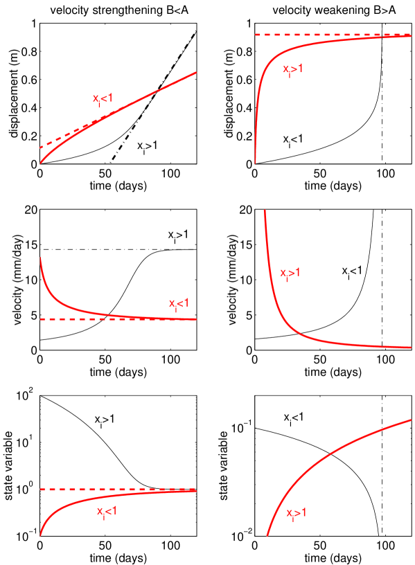
Figure 1: Schematic classification of the different regimes of sliding discussed in the text. The left column of three panels correspond to the stable regime $m=B/A<1$ and the right column of three panels describes the unstable regime $m=B/A>1$. In each case, the displacement, velocity and state variables are shown as a function of time. Each regime (stable and unstable) is divided into two cases, depending on the dimensionless initial value $x_{i}\propto\theta_{i}$ of the state variable. The thick lines corresponds to decreasing velocities and increasing state variables. The thin lines correspond to increasing velocities and decreasing state variables.

The block sliding displays different regimes as a function of the friction law parameters and of the initial conditions. These regimes are controlled by the value of the friction law parameters, i.e., the parameter $m=B/A$, the initial value $x_{i}$ of the reduced state variable and the material parameter $S$ defined by (14). $A$ and $B$ are defined in (3) and are determined by material properties. $x_{i}$ is defined in (17) and is proportional to the initial value of the state variable $\theta$. The parameter $S$ is independent of the initial conditions. As derived from the complete solution in Appendix A, the different regimes are summarized below and in Table 1 and illustrated in Figure 1.

• For $0<m<1$ the sliding is always stable. Depending of the initial value for $t=0$ of the reduced state variable $x_{i}$, the sliding velocity either increases (if $x_{i}>1$) or decreases (if $x_{i}<1$) toward a constant value.

• For $m>1$ the sliding is always unstable. When $x_{i}<1$, the sliding velocity increases toward a finite-time singularity. The slip velocity diverges as $1/(t_{c}-t)$ corresponding to a logarithmic singularity of the cumulative slip. For $x_{i}>1$, the velocity decreases toward a vanishingly small value.

2.4 Analysis of landslide observations, , applications to landslide behaviors

In the sequel, we test how this model can reproduce the observed acceleration of the displacement for Vaiont and La Clapière landslides. The Vaiont landslide was the catastrophic culmination of an accelerated slope velocity over a two months period [Muller, 1964]. La Clapière landslide was characterized by a long lasting acceleration that peaked up in the 1986-1988 period, succeeded by a restabilizing phase [Susella and Zanolini, 1996]. An acceleration of the displacement can arise from the friction model in two regimes, either in the stable regime with $m<1$ and $x_{i}>1$ or in the unstable regime with $m>1$ and $x_{i}<1$. In the first case, the acceleration evolves toward a stable sliding. In the unstable case, the acceleration leads to a finite-time singularity of the displacement and of the velocity. However, these two regimes are very similar in the early time regime before the critical time (see Figure 1). It is therefore very difficult to distinguish from limited observations a landslide in the stable regime from a landslide in the unstable regime when far from the rupture.

We assume that the friction law parameters, the geometry of the landslide and the gravity forces are constant. Within this conceptual model, the complexity of the landsliding behavior emerges from the friction law. We are aware of neglecting in this first order analysis any possible complexity inherent either to the geometry and rheology of a larger set of blocks, or the geometry and rheology of the substratum or the history of the external loading (e.g. earthquake, rainfalls). We invert the friction law parameters from the velocity and displacement data of the Vaiont and La Clapière landslides. Our goal is (i) to test if this model is useful for distinguishing an unstable accelerating sliding characterized by $B>A$ from a stable accelerating regime occurring for $B<A$ and (ii) to test the predictive skills of this model and compare with other methods of prediction.

3 The Vaiont landslide

3.1 Historical and geo-mechanical overview

On the Mt Toc slope in the Dolomite region in the Italian Alps about 100 km north of Venice, on October 9, 1963, a 2 km-wide landslide was initiated at an elevation of 1100-1200 m, that is 500-600 m above the valley floor. The event ended 70 days later in a 20 m/s run-away of about 0.3 km³ of rocks sliding into a dam reservoir. The high velocity of the slide triggered a water surge within the reservoir, overtopping the dam and killing 2500 people in the villages (Longarone, Pirago, Villanova, Rivalta and Fae) downstream.

This landslide has a rather complex history. The landslide occured on the mountain above a newly built dam reservoir. The first attempt to fill up the reservoir was made between March and November 1960. It induced recurrent observations of creeping motions of a large mass of rock above the reservoir, and led to several small and rather slow slides [Muller, 1964]. Lowering the reservoir water level induced the rock mass velocities to drop from $\sim 40$ mm/day to $<1$ mm/day. A controlled raising of the water level as well as cycling were performed. A second peak of creeping velocity, at about 10 mm/day was induced by the 1962 filling cycle. The 1963 filling cycle started in April. From May, recurrent increases of the creep velocity were measured using 4 benchmarks. On september 26, 1963, lowering the reservoir level was again initiated. Contrary to what happened in 1960 and again in 1962, the velocities continued to increase at an increasing rate. This culminated in the $20$ m/s downward movement of a volume of 0.3 km³ of rock in the reservoir.

The landslide geometry is a rough rectangular shape, 2 km wide and 1.3 km in length. Velocity measurements are available for four benchmarks, corresponding to four different positions on the mountain slope, respectively denoted 5, 50, 63 and 67 in the Vaiont nomenclature. Benchmarks 63 and 67 are located at the same elevation in the upper part of the landslide a few hundred meters from the submittal scarp. The distance between the two benchmarks is 1.1 km. The benchmark 5 and 50 are 700 m downward the 63-67 benchmark level.

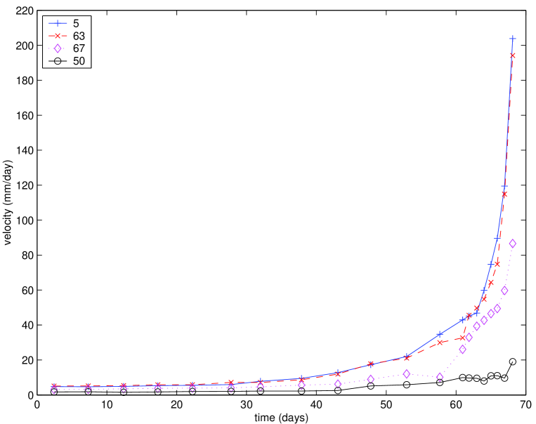
Figure 2: Velocity measurements for the four benchmarks of the Vaiont landslide. Benchmarks 5 and 63 exhibit similar acceleration. Benchmark 50 shows only a relatively small acceleration in absolute values at the end of the 60 days accelerating phase. Its acceleration is however significant in relative values, as seen in Figure 4. Data from [Muller, 1964].

Figure 2 shows the velocity of the four benchmarks on the block as a function of time prior to the Vaiont landslide. For these four benchmarks, the deformation of the sliding zone prior to rupture is not homogeneous, as the cumulative displacement in the period from August 2^nd, 1963 to October 8, 1963 ranges from 0.8 to 4 m. However, the low degree of disintegration of the distal deposit [Erismann and Abele, 2000] argue for a possible homogeneous block behavior during the 1963 sliding collapse.

It was recognized later that limestones and clay beds dipping into the valley provide conditions favorable for dip-slope failures [Muller, 1964, 1968; Broili, 1967]. There is now a general agreement on the collapse history of the 1963 Vaiont landslide (see e.g., [Erismann and Abele, 2000]). The failure occurred along bands of clays within the limestone mass at depths between 100-200 m below the surface [Hendron and Patton, 1985]. Raising the reservoir level increased water pore pressure in the slope flank, that triggered failure in the clays layers. Final sliding occurred after 70 days of down-slope accelerating movement. The rock mass velocity progressively increased from 5 mm/day to more than 20 cm/day, corresponding to a cumulative displacement of a few meters over this 70 days period [Muller, 1964].

3.2 Analysis of the velocity data with the slider-block model parameters.

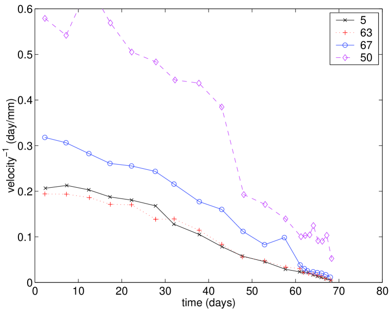
Figure 3: Same as Figure 2 by plotting the inverse of the velocity as a time $t$. All curves are roughly linear, showing that the velocity exhibits a finite-time singularity $v\sim 1/(t_{c}-t)$ with $t_{c}\approx 69.5$ days for all benchmarks, estimated as the intercept of the extrapolation of these curves with the horizontal axis.

Figure 3 shows the inverse of the velocity shown in Figure 2 to test the finite-time-singularity hypothesis (2,11). Note that this figure does not require the knowledge of the critical time $t_{c}$ and is not a fit to the data. The curves for all benchmarks are roughly linear in this representation, in agreement with a finite-time singularity of the velocity (2) with $\alpha=2$. It was the observations presented in Figure 3 that led Voight to suggest that a prediction could have been issued more than 10 days before the collapse [Voight, 1988]. We note that the law $\dot{\delta}\propto 1/(t_{c}-t)$ requires the adjustment of $\alpha$ to the special value $2$ in the phenomenological approach [Voight, 1988] underlying (2) while it is a robust and universal result in our model leading to (11) in the velocity-weakening regime $B>A$, $m>1$ and for a normalized initial state variable larger than $1$ (see equation (11) and Table 1).

In order to invert the parameters $m$, $D$, $T$ of the friction model and the initial condition of the state variable $x_{i}$ from the velocity data, we minimize the $rms$ (root-mean-square) of the residual between the observed velocity $\dot{\delta}_{obs}$ and the velocity $\dot{\delta}$ from the friction model (20) and (19). The constant $D$ in (19) is obtained by taking the derivative of the $rms$ with respect to $D$, which yields

$$D={\sum_{t_{i}}\dot{\delta}(t_{i})\dot{\delta}_{obs}(t_{i})\over\sum_{t_{i}}{\dot{\delta}(t_{i})}^{2}}$$ (12)

where the velocity $\dot{\delta}$ in (12) is evaluated for $D=1$ in (19). We use a simplex algorithm (matlab subroutine) to invert the three other parameters. For each data set, we use different starting points (initial parameter values for the simplex algorithm) in the inversion to test for the sensitivity of the results on the starting point.

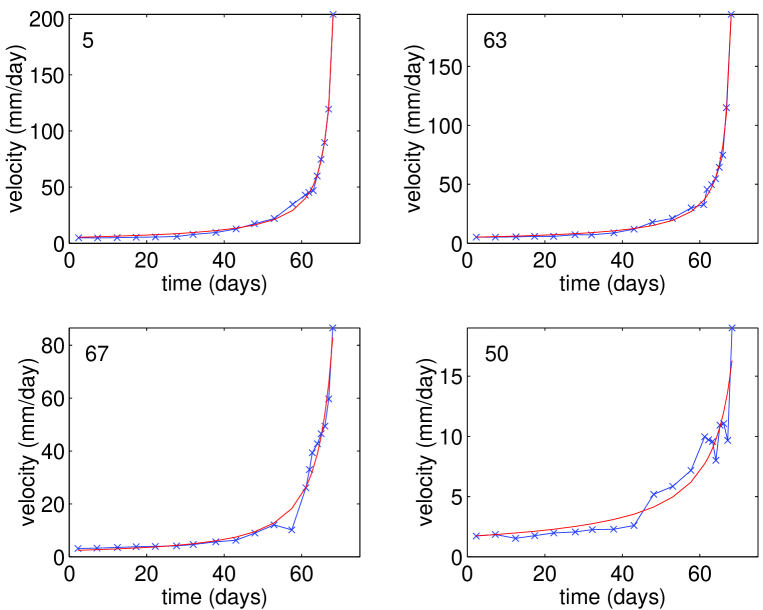
Figure 4: For each of the four Vaiont benchmarks, the velocity data of Figure 2 is fitted with the slider-block model with the state and velocity friction law (20) and (19) by adjusting the set of parameters $m$, $D$, $T$ and the initial condition of the state variable $x_{i}$. The data are shown as the crosses linked by straight segments and the fit is the thin continuous line. The fitted $m$ are respectively $m=1.35$ (benchmark 5), $m=1.24$ (benchmark 63), $m=0.99$ (benchmark 67) and $m=1.00$ (benchmark 50).

Figure 4 shows the fits to the velocity data using the slider-block model with the state and velocity friction law (19) and (20). The values of $m=B/A$ are respectively $m=1.35$ (benchmark 5), $m=1.24$ (benchmark 63), $m=0.99$ (benchmark 67) and $m=1.00$ (benchmark 50). Most values are larger than or equal to $1$, which is compatible with the finite-time-singularity regime summarized in Table 1. The parameters of the friction law are very poorly constrained by the inversion. In particular, even for those benchmarks were the best fit gives $m>1$, other models with $m<1$ provide a good fit to the velocity with only slightly larger rms.

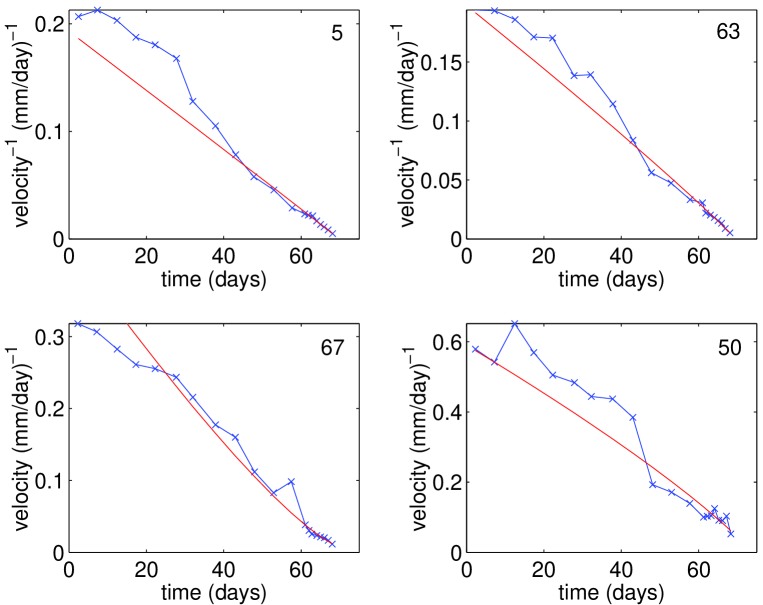
Figure 5: Same as Figure 4 but showing the inverse of the velocity. The upward bending of the curve for benchmark 67 reflects the saturation of the velocity in the stable regime $B<A$. The fit for the three other benchmarks characterized by $m\geq 1$ is very close to the asymptotic solution $v\sim 1/(t_{c}-t)$ (11).

Figure 5 gives another representation of Figure 4 showing the inverse of the velocity as a function of time. The increase of velocity seems to be exhausted before the critical time for all benchmarks, which may explain the values $m<1$ sometimes obtained by the inversion.

4 La Clapière landslide: the aborted 1982-1987 acceleration

We now report results on another case which exhibited a transient acceleration which did not result in a catastrophic failure but re-stabilized. This example provides what is maybe an example of the $m<1$ stable slip regime, i.e. $B<A$, as interpreted within the friction model.

4.1 Historical and geo-mechanical overview

4.1.1 Geo-mechanical setting and Displacement history: 1950-2000

La Clapière landslide is located at an elevation between 1100 m and 1800 m on a 3000m high slope. The landslide has a width of about 1000 m. Figure 6 shows La Clapière landslide in 1979 before the acceleration of the displacement, and in 1999 after the end of the crisis. The volume of mostly gneiss rocks implied in the landslide is estimated to be around $50\times 10^{6}$ m³. At an elevation of about 1300 m, a 80 m thick bed provides a more massive and relatively stronger level compared with the rest of relatively weak and fractured gneiss. The two lithological entities are characterized by a change in mica content which is associated with a change of the peak strength and of the elastic modulus by a factor two [Follacci et al., 1990, 1993]. Geomorphological criteria allow one to distinguish three distinct sub-entities within the landslide, NW, Central and SW respectively [Follacci et al., 1988].

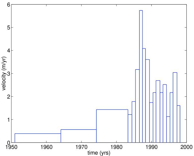
Figure 7: Velocity of the landslide of La Clapière mount over almost 50 years, showing that the dangerous velocity peak in 1987 was preceded by a progressing build-up extending over several decades. Before 1982, the velocity is inferred from aerial photographs in 1951, 1964, 1974 and 1982. After 1982, the velocity is obtained from automated triangulation and geodesy. Data from CETE [1999].

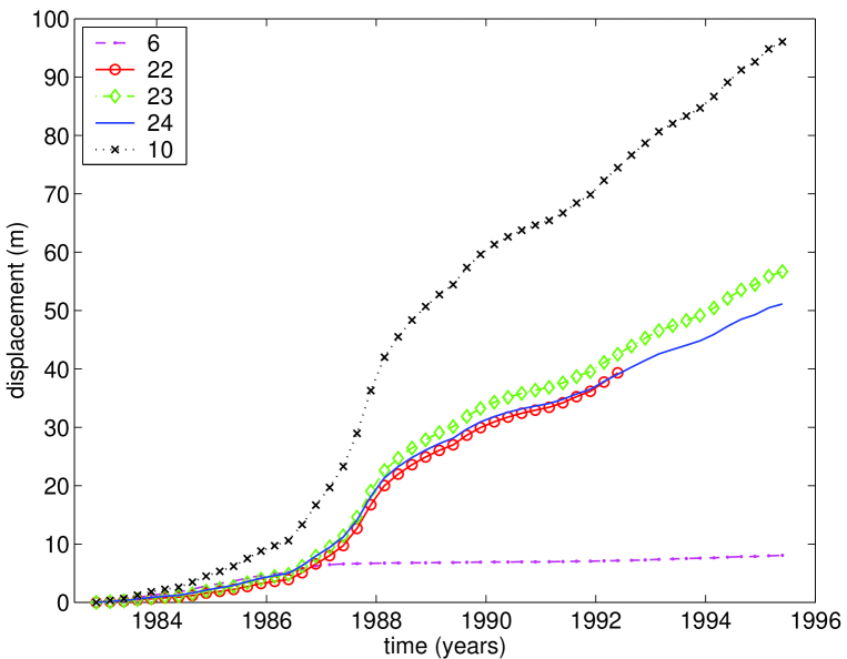
Figure 8: Displacement for the 5 benchmarks on La Clapière site shown in Figure 6.

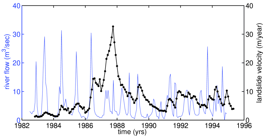
Figure 9: Velocity pattern for benchmark 10 of La Clapière landslide (solid line and dots) and flow rates (thin solid line) of the Tinée river on the 1982-1995 period. Because the Tinée river runs at the basis of La Clapière landslide, the river flow rate reflects the water flow within the landslide [Follacci et al., 1993; Susella and Zanolini, 1996]. The flow rates are measured at St Etienne village, 2 km upstream the landslide site. There is no stream network on the landslide site. The Tinée flow drains a 170 km² basin. This tiny basin is homogeneous both in terms of slopes and elevation (in the 1000-3000 m range). Accordingly, the seasonal fluctuations of the river flow reflects the amount of water within the landslide slope due to rainfalls and snow melting. Data from CETE [1996].

There is some historical evidence that the rock mass started to be active before the beginning of the 20th century. In 1938, photographic documents attest the existence of a scarp at 1700 m elevation [Follacci, 2000]. In the 1950-1980 period, triangulation and aerial photogrametric surveys provide constraints on the evolution of the geometry and the kinematics of the landslide (Figure 7). The displacement rate measured by aerial photogrametric survey increased from 0.5 m/yrs in the 1950-1960 period to 1.5 m/yrs in the 1975-1982 period [Follacci et al., 1988]. Starting in 1982, the displacements of 43 benchmarks have been monitored on a monthly basis using distance meters (using a motorised theodolite (TM300) and a Wild DI 3000 distance meter) [Follacci et al., 1988, 1993; Susella and Zanolini, 1996]. The displacement data for the 5 benchmarks in Figure 6 is shown in Figure 8. The velocity of benchmark 10, which is typical, is shown in Figure 9. The rock mass velocities exhibited a dramatic increase between January 1986 and January 1988, that culminated in the 80 mm/day velocity during the 1987 summer and to 90 mm/day in October 1987. The homogeneity of benchmark trajectories and the synchronous acceleration phase for most benchmark, attest of a global deep seated behavior of this landslide [e.g. Follacci et al., 1988]. However, a partitioning of deformation occurred, as reflected by the difference in absolute values of benchmark displacements (Figure 8). The upper part of the landslide moved slightly faster than the lower part and the NW block. The observed decrease in displacement rate since 1988 attest of a change in landsliding regime at the end of 1987 (Figure 8) .

4.1.2 Correlations between the landslide velocity and the river flow

The landslide velocity displays large fluctuations correlated with fluctuations of the river flow in the valley as shown in Figure 9. There is a seasonal increase of the slope velocity which reaches a maximum $V_{\rm max}$ of the order of or less than $30$ mm/days. The slope velocity increases in the spring due to snow melting and over a few days after heavy precipitations concentrated in the fall of each year [Follacci et al., 1988; Susella and Zanolini, 1996]. During the 1986-1988 period, the snow melt and rainfalls were not anomalously high but the maximum value of the velocity, $V_{\rm max}=90$ mm/day, was much larger that the velocities reached during the 1982-1985 period for comparable rainfalls and river flows [Follacci et al., 1988; 1993]. This strongly suggests that the hydrological conditions are not the sole control parameters explaining both the strong 1986-1987 accelerating and the equally strong slowdown in 1988-1990. During the interval 1988-1990, the monthly recorded velocities slowed down to a level slightly higher than the pre-1986 values. Since 1988, the seasonal variations of the average velocity never recovered the level established during the 1982-1985 period [Follacci et al., 1993; David and ATM, 2000]. Rat [1988] derives a relationship between the river flow and the landslide velocity by adjusting an hydrological model to the velocity data in the period 1982 to 1986. This model tuned to this time period does not reproduce the observed acceleration of the velocity after 1986.

4.1.3 Fracturing patterns contemporary to the 1986-1987 accelerating regime

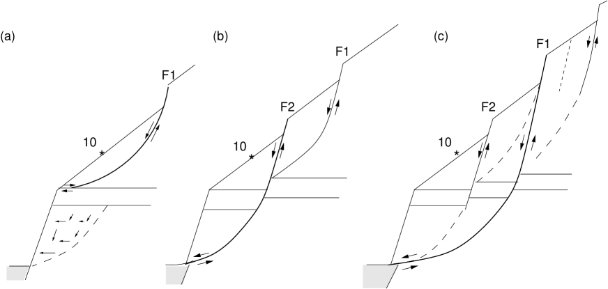
Figure 10: Schematic structural interpretation of one possible mechanism involved in the 1986-1988 crisis. The 3 schematic cross sections are the proposed landslide geometries, before 1986 (a), during the 1987 acceleration (b), and after 1988 (c). Follacci et al. [1993] argue for the failure of the strong gneiss bed (F2 fault) in the NW block as the driving force behind the 1986-1987 accelerating phase (b). In the same period, the development of the upper NW crack, (F1 fault on central cross section), that released the landslide from its head driving force, appears as the key parameter to slow down the accelerating slide. Guglielmi and Vengeon. [2002] argue for all the surface faulting patterns to converge at shallow depth as listric faults that define a decollement level which is the sliding surface. The star shows the location of benchmark 10 (adapted from [Follacci et al., 1993]).

In 1985-1986, a transverse crack initiated in the upper part of the NW block. It reaches 50 m of vertical offset in 1989. The maximum rate of change of the fracture size and of its opening occurred in 1987 [Follacci et al., 1993]. This new transverse crack uncoupled the NW block from the upper part of the mountain, which moved at a much smaller velocity below 1 mm/day since 1985-86 [Follacci et al., 1993] (Figures 6 and 10). Since summer 1988, an homogenization of the surface morphological faces and a regression of the main summit scarp were reported. The regression of the summit scarp was observed as a new crack started to open in September 1988. Its length increased steadily to reach 500 m and its width reached 1.75 m in November 1988. Accordingly, the new elevation of main scarp in the SE block reaches 1780 m. This crack, which defined a new entity, that is the upper SE block, has remained locked since then (Figures 6 and 10).

4.1.4 Current understanding of La Clapière acceleration

On the basis of these observations and simple numerical models, an interpretative model for the 1986-1988 regime change was proposed by Follacci et al., [1993] [see also for a review Susella and Zanolini, 1996]. In fact, these models do not explain the origin of the acceleration but rather try to rationalize kinematically the different changes of velocity and why the acceleration did not lead to a catastrophic sliding but re-stabilized. The reasoning is based on the fact that the existing and rather strong correlation between the river flow in the valley at the bottom and the slope motion (see Figure 9) is not sufficient to explain both the de-stabilizing phase and its re-stabilization. This strongly suggests that the hydrological conditions are not the sole control parameters explaining both the strong 1986-1987 accelerating and the equally strong slowdown in 1988-1990.

Follacci et al. [1988, 1993] argue that the failure of the strong gneiss bed in the NW block was the main driving force of the acceleration in 1986-1987. According to this view, the failure of this bed induced changes in both the mechanical boundary conditions and in the local hydro-geological setting (Figure 10). Simultaneously, the development of the upper NW crack, that freed the landslide from its main driving force, appears as a key parameter to slow down the accelerating slide. The hypothesized changes in hydrological boundary conditions can further stabilize the slide after the 1986-1987 transient acceleration.

Several works have attempted to fit the velocity time series of La Clapière landslide and predict its future evolution, using a framework similar to the Vaiont landslide discussed above. The displacement of different benchmarks over the 1982-1986 period has been analysed. An exponential law has been fitted to the 1985-1986 period [Vibert et al., 1988]. Using the exponential fit and a failure criterion that the landslide will collapse when the velocity reaches a given threshold, the predicted collapse time for the landslide ranges from 1988 for NW benchmark to 1990 for the SE benchmarks. Plotting the inverse of the velocity as a function of time as in (2) has been tried, hoping that this law holds with $\alpha=2$ providing a straightforward estimation of $t_{c}$. This approach applied to La Clapière velocity data predicts a collapse in 1990 for the upper NW part and in 1988-1989 for the SE part of the landslide. To remove the fluctuations of the velocity induced by changes in river flow, an ad-hoc weighting of the velocity data was used by [Vibert et al., 1988]. An attempt to more quantitatively estimate the relation between the river flow and the landslide velocity was proposed by Rat [1988]. Rat [1988] stresses the importance of removing the fluctuations of the velocity induced by changes in the river flow before any attempt to predict the collapse time.

4.2 Analysis of the cumulative displacement and velocity data with the slider-block model

4.2.1 La Clapière sliding regime: 1982-1987

We fit the monthly measurements of the displacement of several representative benchmarks with the slider-block friction model. In the sequel, we will show results for benchmark 10 which is located in the central part of the landslide (Figure 6), and which is representative of the average landslide behavior during the 1982-1995 period [Follacci, personal communication 2001]. We have also obtained similar results for benchmark 22.

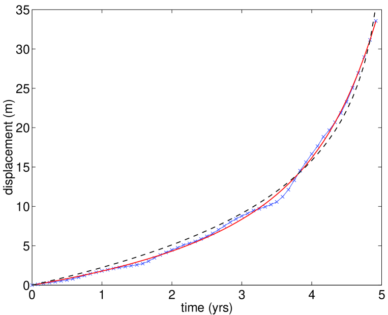
Figure 11: Displacement for benchmark 10 of la Clapière landslide (crosses) and fit using the friction model. The best fit gives $m=0.98$ (black line). The dashed line shows the best fit obtained when imposing $m=1.5$ for comparison.

We consider only the accelerating phase in the time interval $[1982.9;1987.9]$. As for the Vaiont landslide, the inversion provides the values of the parameters $m$, $T$, $D$, and the initial condition $x_{i}$ of the state variable. For La Clapière, we analyze the displacement as it has a lower noise level compared with the velocity. In the Vaiont case, the data is of sufficiently good quality to use the velocity time series which allows us to compare with previous studies. The best fit to the displacement of benchmark 10 is shown in Figure 11. The model parameters are $m=B/A$=0.98 and the initial value of the reduced state variable is $x_{i}=39$. While $m$ is very close to one, the value of $x_{i}$ significantly larger than 1 argues for La Clapière landslide to be in the stable regime (see Figure 1 and Table 1). Similar results are obtained for the other benchmarks. Since the landslide underwent different regimes, it is important to perform these inversions for different time periods, that is, the fits are done from the first measurement denoted time $t=0$ (year $1982.9$) to a later $t=t_{\rm max}$, where $t_{\rm max}$ is increased from approximately $2$ years to $5$ years after the initial starting date. This last time $t\approx 5$ years (end of 1987) corresponds to the time at which the slope velocity reached its peak. For all inversions except the first two point with $t_{\rm max}\approx 2$ yrs, the best fit always select an exponent $0<m<1$ and an initial state variable $x_{i}\gg 1$, corresponding to a stable asymptotic sliding without finite-time singularity. For $t_{\rm max}<4$ years (that is, using data before the end of 1986), a few secondary best solutions are found with very different values, from $m=-3000$ to $m=29$, indicating that $m$ is poorly constrained. We have also performed sensitivity tests using synthetic data sets generated with the friction model with the same parameters as those obtained for La Clapière. These tests show that a precise determination of $m$ is impossible but that the inversion recovers the true regime $m<1$.

The transition time (defined by the inflection point of the velocity) is found to increase with $t_{max}$. This may argue for a change of regime from an acceleration regime to a restabilization before the time $t=1988$ of the velocity peak. The parameters $S$ and $x_{i}$ are also poorly constrained. Similar results are obtained for different benchmarks as well as when fitting the velocity data instead of the displacement [Helmstetter, 2002; Sornette et al.,2003]. The velocity data show large fluctuations, in part due to yearly fluctuations of the precipitations. The inversion is therefore even more unstable than the inversion of the displacement, but almost all points give $m<1$ and $x_{i}>1$. Such fluctuations of the inverted solution may indicate that the use of constant friction parameters to describe a period where 2 regimes interact, i.e., an accelerating phase up to 1987 followed by a decrease in sliding rate since 1988, does not describe adequately the landslide behavior for the whole time period 1982-1996. Observed changes in morphology as suggested in Figures 6 and 10 provide evidence for changes both in driving forces and in the geometry of the landslide, including possible new sliding surfaces.

4.2.2 La Clapière decelerating phase: 1988-1996

The simple rigid block model defined with a single block and with velocity and state dependent friction law cannot account for what happened after the velocity peak, without invoking additional ingredients. Departure from the model prediction can be used as a guide to infer in-situ landslide behavior. Recall that, during the interval 1988-1990, the monthly recorded velocities slowed down to velocity 6 times smaller than the 1987 peak values. This deceleration cannot be explained with the friction model using constant friction parameters. Indeed, for $B/A=m<1$, under a constant geometry and fixed boundary conditions, the velocity increases and then saturates at its maximum value. In order to explain the deceleration of the landslide, a change of material properties can be invoked (embodied for example in the parameter $m=B/A$) or a change of the state variable $\theta$ that describes the duration of frictional contacts, maybe due to a change in the sliding surfaces.

We have not attempted in this study to fit both the accelerating and the decelerating phases with the slider-block model due to the large number of free parameters it will imply relatively to the small number of points available. Further modeling would allow block partitioning, fluctuations of the slope angle and change with time of the friction parameters. Our purpose is here to point out how different landsliding regimes can be highlighted by the introduction of a velocity and state friction law in this basic rigid block model.

5 Discussion and conclusion

We have presented a quantitative analysis of the displacement history for two landslides, Vaiont and La Clapière, using a slider-block friction model. An innovative concept proposed here was to apply to landslides the state and velocity dependent friction law established in the laboratory and used to model earthquake friction. Our inversion of this simple slider-block friction model shows that the observed movements can be well reproduced with this simple model and suggest the Vaiont landslide (respectively La Clapière landslide) as belonging to the velocity weakening unstable (respectively strengthening stable) regime. Our friction model assumes that the material properties embodied in the key parameters $m=B/A$ and/or the initial value of the state variable of the friction law control the sliding regime.

Our purpose was here to point out how different landsliding regimes can be highlighted by the introduction of a velocity and state friction law in a basic rigid block model. Even if the displacement is not homogeneous for the two landslides, the rigid block model provides a good fit to the observations and a first step towards a better understanding of the different sliding regimes and the potential for their prediction.

For the cases studied here, we show that a power law increase with time of of the slip velocity can be reproduced by a rigid slider block model. This first order model rationalizes the previous empirical law suggested by Voight [1988]. Following Petley et al. [2002], we suggest that the landslide power law acceleration emerges in the presence of a rigid block, i.e., this corresponds to the slide of a relatively stiff material. Petley et al. [2002] report that, for some other types of landslides in ductile material, the slips do not follow a linear dependence with time of the inverse landslide velocities. They suggest that the latter cases are reminiscent of the signature of landsliding associated with a ductile failure in which crack growth does not occur. In contrast, they proposed that the linear dependence of the inverse velocity of the landslide as a function of time is reminiscent of crack propagation, i.e., brittle deformation on the basal shear plane. Our contribution suggests that friction is another possible process that can reproduce the same accelerating pattern than the one proposed to be driven by crack growth on a basal shear plane [Petley et al., 2002; Kilburn and Petley, 2003]. The friction model used in our study requires the existence of an interface. Whether this friction law should change for ductile material is not clear. The lack of direct observations of the shearing zone and its evolution through time makes difficult the task of choosing between the two classes of models, crack growth versus state-and-velocity-dependent friction. We recover here the still on-going debate for earthquakes, which can be seen as either frictional or faulting events.

For the Vaiont landslide, this physically-based model suggests that this landslide was in the unstable regime. For La Clapière landslide, the inversion of the displacement data for the accelerating phase 1982-1887 up to the maximum of the velocity gives $m<1$, corresponding to the stable regime. The deceleration observed after 1988 implies that, not only is La Clapière landslide in the stable regime but in addition, some parameters of the friction law have changed, resulting in a change of sliding regime from a stable regime to another one characterized by a smaller velocity, as if some stabilizing process or reduction in stress was occurring. Possible candidates for a change in landsliding regime include the average dip slope angle, the partitioning of blocks, new sliding surfaces and changes in interface properties. The major innovation of the frictional slider-block model which is explored further in [Sornette et al., 2003] is to embody the two regimes (stable versus unstable) in the same physically-based framework, and to offer a way of distinguishing empirically between the two regimes, as shown by our analysis of the two cases provided by the Vaiont and La Clapière landslides.

We thanks C. Scavia and Y. Guglielmi for key supports to capture archive data for Vaiont and La Clapière landslide respectively. We are very grateful to N. Beeler, J. Dieterich, Y. Guglielmi, D. Keefer, J.P. Follacci, J.M. Vengeon for useful suggestions and discussions. AH and JRG were supported by INSU french grants, Gravitationnal Instability ACI. SG and DS acknowledge support from the James S. Mc Donnell Foundation 21st century scientist award/studying complex systems.

Appendix A Appendix A: Derivation of the full solution of the frictional problem

We now provide the full solution of the frictional problem. First, we rewrite (3) as

$$\dot{\delta}=S~{}D_{c}~{}\left({\theta\over\theta_{0}}\right)^{-m}~{},$$ (13)

where

$$S\equiv{\dot{\delta}_{0}~{}e^{{\tau\over\sigma}-\mu_{0}\over A}\over D_{c}}$$ (14)

and

$$m\equiv{B\over A}~{}.$$ (15)

Putting (13) in (4) gives

$${{\rm d}(\theta/\theta_{0})\over{\rm d}t}={1\over\theta_{0}}-S~{}(\theta/\theta_{0})^{1-m}~{}.$$ (16)

The case $m=1$ requires a special treatment since the dependence in $\theta$ disappears in the right-hand-side of (16) and ${{\rm d}\theta\over{\rm d}t}$ is constant.

For $m\neq 1$, it is convenient to introduce the reduced variables

$$x\equiv(S\theta_{0})^{1/(1-m)}~{}{\theta\over\theta_{0}}~{},$$ (17)

and

$$D\equiv D_{c}~{}\left(S\theta_{0}^{m}\right)^{1\over 1-m}~{}.$$ (18)

Then, (13) reads

$${\dot{\delta}\over\dot{\delta}_{0}}=D~{}x^{-m}~{}.$$ (19)

Putting (13) in (4) to eliminate the dependence in $\dot{\delta}$, we obtain

$${{\rm d}x\over{\rm d}t^{\prime}}=1-x^{1-m}~{},$$ (20)

where $t^{\prime}=t/T$ with

$$T={D_{c}\over D}=\left[{D_{c}\over\dot{\delta}_{0}\theta_{0}^{m}}\right]^{1/(1-m)}~{}e^{{\tau\over\sigma}-\mu_{0}\over B-A}~{}.$$ (21)

In the sequel, we shall drop the prime and use the dimensionless time $t^{\prime}$, meaning that time is expressed in units of $T$ except stated otherwise.

The block sliding behavior is determined by first solving the equation (20) for the normalized state variable $x(t)$ and then by inserting this solution in (19) to get the slip velocity. Equation (20) displays different regimes as a function of $m$ and of the initial value $x_{i}$ compared to $1$ that we now classify.

A.1 Case $m=B/A>1$

For $m>1$ and $x_{i}<1$, the initial rate of change ${{\rm d}x\over{\rm d}t}$ of the state variable is negative. The initial decay of $x$ accelerates with time and $x$ reaches $0$ in finite time. Expression (19) shows that $\delta(t)$ continuously accelerates and reaches infinity in finite time. Close to the singularity, we can neglect the first term $1$ in the right-hand-side of (20) and we recover the asymptotic solution (9,10,11):

$$x(t)\simeq m^{1\over m}~{}(t_{c}-t)^{1\over m}~{},$$ (22)

where the critical time $t_{c}$ is determined by the initial condition $x(t=0)=x_{i}$

$$t_{c}={x_{i}^{m}\over m}~{}.$$ (23)

For $m>1$ and $x_{i}>1$, the initial rate of change ${{\rm d}x\over{\rm d}t}$ of the state variable is positive, thus $x$ initially increases. This growth goes on, fed by the positive feedback embodied in (20). At large times, $x$ increases asymptotically at the constant rate ${{\rm d}x\over{\rm d}t}=1$ leading to $x(t)\approx t$. Integrating equation (19) gives

$$\delta(t)=\delta_{\infty}-{\dot{\delta}_{0}D\over m-1}~{}{1\over t^{m-1}}~{},$$ (24)

at large times. The asymptotic value of the displacement $\delta_{\infty}$ is determined by the initial condition. This regime thus describes a decelerating slip slowing down as an inverse power of time. It does not correspond to a de-stabilizing landslide but to a power law plasticity hardening.

A.2 Case $m=B/A=1$

In this case, the variables (17) and (18) are not defined and we go back to (4) (which uses the unnormalized state variable $\theta$ and time $t$) to obtain

$${{\rm d}\theta\over{\rm d}t}=1-S\theta_{0}~{},$$ (25)

where $S$ is defined by (14) and depends on the material properties but not on the initial conditions. If $S\theta_{0}>1$, $\theta$ decays linearly and reaches $0$ in finite time. This retrieves the finite-time singularity, with the slip velocity diverging as $1/(t_{c}-t)$ corresponding to a logarithmic singularity of the cumulative slip. If $S\theta_{0}<1$, $\theta$ increases linearly with time. As a consequence, the slip velocity decays as $\dot{\delta}\sim 1/t$ at large times and the cumulative slip grows asymptotically logarithmically as $\ln t$. This corresponds to a standard plastic hardening behavior.

A.3 Case $m=B/A<1$

For $x_{i}>1$, the initial rate of change ${{\rm d}x\over{\rm d}t}$ of the state variable is negative, thus $x$ decreases and converges to the stable fixed point $x=1$ exponentially as

$$x=1+ae^{-{t\over t^{*}}}~{},$$ (26)

where the relaxation time $t^{*}$ is given by

$$t^{*}={1\over 1-m}$$ (27)

in units of $T$ and $a$ is a constant determined by the initial condition. Starting from some initial value, the slip velocity increases for $0<m<1$ (respectively decreases for $m<0$) and converges to a constant, according to (13,19).

For $x_{i}<1$, the initial rate of change ${{\rm d}x\over{\rm d}t}$ of the state variable is positive, and $x$ converges exponentially toward the asymptotic stable fixed point $x=1$. As $\theta$ increases toward a fixed value, this implies that the slip velocity decreases for $0<m<1$ (respectively increases for $m<0$) toward a constant value.

Anifrani, J.-C., C. Le Floch, D. Sornette and B. Souillard, Universal Log-periodic correction to renormalization group scaling for rupture stress prediction from acoustic emissions, J. Phys. I France 5, 631-638, 1995.

Bhandari, R. K, Some lessons in the investigation and field monitoring of landslides, Proceedings 5th Int. Symp. Landslides Lausanne 1988, eds C. Bonnard , 3, 1435-1457, Balkema, 1988.

Blanpied, M. L., D. A. Lockner and J. D. Byerlee, Frictional slip of granite at hydrothermal conditions, J. Geophys. Res., 100, 13045-13064, 1995.

Broili, L., New knowledge on the geomorphology of the Vaiont slide slip surfaces, Rock mechanics and Engineering, 5, 38-88, 1967.

Campbell, C.S., Self-lubrification for long runout landslides, Journal of Geology, 97, 653-665, 1989.

Campbell, C.S., Rapid granular flow, Annu. Rev. of Fluid Mech., 22, 57-92, 1990.

Caplan-Auerbach, J., C. G. Fox and F. K. Duennebier, Hydroacoustic detection of submarine landslides on Kilauea volcano, Geophys. Res. Letts, 28, 1811-1813, 2001.

David, E. and ATM, Glissement de La Clapière, St Etienne de Tinée, Etude cinématique, géomorphologique et de stabilité, rapport CETE Nice, France, 88 pp., 2000.

Davis, R.O., N. R. Smith and G. Salt, Pore fluid frictional heating and stability of creeping landslides, Int. J. Num. Anal. Meth. Geomechanics, 14, 427-443, 1990.

Dieterich, J., Time dependent friction and the mechanics of stick slip, Pure Appl. Geophys., 116, 790-806, 1978.

Dieterich, J. H., Earthquake nucleation on faults with rate- and state-dependent strength, Tectonophysics, 211, 115-134, 1992.

Durville, J.L., Study of mechanisms and modeling of large slope movements, Bull. Int. Ass. Engineering Geology, 45, 25-42, 1992.

Eisbacher, G.H., Cliff collapse and rock avalanches in the Mackenzie Mountains, Northwestern Canada, Can. Geot. J., 16, 309-334, 1979.

Erismann, T.H. and G. Abele, Dynamics of Rockslides and Rockfalls, Springer, 300 pp, 2000.

Follacci, J. P., Photographic album of La Clapière landslide, CETE Méditerranée, 2000.

Follacci, J. P., P. Guardia and J. P. Ivaldi, La Clapière landslide in its geodynamical setting, Bonnard eds , Proc. 5th Int. Symp. on Landslides, 3, 1323-1327, 1988.

Follacci, J.-P., L. Rochet and J.-F. Serratrice, Glissement de La Clapière, St Etienne de Tinée, Synthèse des connaissances et actualisation des risques, rapport 92/PP/UN/I/DRM/03/AI/01, Ministère Environnement, 76 pp., 1993.

Fruneau, B., J. Achache and C. Delacourt, Observation and modeling of the Saint-Etienne-de-Tinée landslide using SAR interferometry, Tectonophysics, 265, 181-190, 1996.

Gluzman, S. and D. Sornette, Self-Consistent theory of rupture by progressive diffuse damage, Physical Review E, 6, 306 N6 PT2:6129,U241-U250, 2001.

Gomberg, J., P. Bodin, W. Savage and M. E. Jackson, Landslide faults and tectonic faults, Analogs? – The slumgullion earthflow, Colorado, Geology, 23, 41-44, 1995.

Gomberg, J., N. Beeler and M. Blanpied, On rate-state and Coulomb failure models, J. Geophys. Res., 105, 7857-7871, 2000.

Guglielmi, J., and J. M. Vengeon, Interrelation between gravitational patterns and structural fractures La Clapière, French Alps, submitted to Geomorphology, 2002.

Helmstetter, H., Rupture and Instabilities: seismicity and landslides, PhD thesis, Grenoble University, pp 387, 2002.

Heim A., Bergsturz and Menschenleben, Zurich, 1932.

Hendron, A. J. and F. D. Patton, The Vaiont slide, a geotechnical analysis based on new geologic observations of the failure surface, US Army Corps of Engineers Technical Report GL-85-5 (2 volumes), 1985.

Hoek, E. and E. T. Brown, Underground excavation in rock, Institution of Mining and Metallurgy, London, 1980.

Hoek, E., and J. W. Bray, Rock slope engineering, 3rd Edn (rev), Institution of Mining and Metallurgy and E&FN Spon, London, pp 358, 1997.

Jaume, S. C. and L. R. Sykes, Evolving toward a critical point: A review of accelerating seismic moment/energy release prior to large and great earthquakes, Pure and Appl. Geophys., 155, 279-305, 1999.

Kennedy B. A. and K. E. Niermeyer, Slope Monitoring systems used in the Prediction of a Major Slope Failure at the Chuquicamata Mine, Chile, Proc. on Planning Open Pit Mines, Johannesburg, Balkema, 215-225, 1971.

Kilburn, C. R. J., and D. N. Petley, Forecasting giant, catastrophic slop collapse: lessons from Vajont, Northern Italy, in press. Geomorphology, 2003.

Korner, H. J., Reichweite and Geschwindigkeit von Bergsturzen und Fleisscheneelawinen, Rock mechanics, 8, 2256-256, 1976.

Malet, J. P., O. Maquaire and E. Calais, The use of Global Positioning System techniques for the continuous monitoring of landslides: application to the Super-Sauze earthflow (Alpes-de-Haute-Provence, France), Geomorphology, 43, 33-54, 2002.

Mantovani, F., R. Soeters and C. J. Vanwesten, Remote sensing techniques for landslide studies and hazard zonation in Europe, Geomorphology, 15, 213-225, 1996.

Marone, C., Laboratory-derived friction laws and their application to seismic faulting, Ann. Rev. Earth Planet. Sci., 26, 643-696, 1998.

Muller L., The rock slide in the Vaiont valley, Felsmechanik und Ingenoirgeologie, 2 (3-4), 148-212, 1964.

Muller L., News consideration on the Vaiont slide, Felsmechanik und Ingenoirgeologie, 6, 1-91, 1968.

Parise, M., Landslide mapping techniques and their use in the assessment of the landslide hazard, Phys. Chem. Earth, Part C- Solar-Terr. Plan. Sci., 26, 697-703, 2001.

Petley, D.N., Bulmer, M.H. and Murphy W. , Patterns of movement in rotational and translational landslides, Geology. 30(8), 719-722, 2002.

Rabotnov, Y. N., Creep problems in Structural Members, North-Holland eds, Amsterdam, 1969.

Rat, M., Difficulties in forseeing failure in landslides - La Clapière, French Alps, Proceedings 5th Int. Symp. Landslides Lausanne 1988, eds C. Bonnard, vol 3, 1503-1504, Balkema, 1988.

Rousseau, N., Study of seismic signals associated with rockfalls at 2 sites on the Reunion island (Mahavel Cascade and Souffrière cavity), PhD thesis, IPG Paris, 1999.

Ruina, A. L., Slip instability and sate variable friction laws, J. Geophys. Res., 88, 10359-10370, 1983.

Saito, M., Forecasting the Time of occurrence of a Slope Failure, Proc. 6th Int. Conf. Soil Mech. & Found. Eng., Montreal, vol.2, 537-541, 1965.

Saito, M., Forecasting time of Slope Failure by Tertiary Creep, Proc. of 7th Int. Conf. Soil Mech. & Found. Eng., Mexico City, vol. 2, 677-683, 1969.

Saito, M. and H. Uezawa, Failure of soil due to creep, Proc of 6th Int. Conf. Soil Mech. & Found. Eng., Montreal, vol. 1, 315-318, 1961.

Sammis, S. G. and D. Sornette, Positive Feedback, Memory and the Predictability of Earthquakes, Proceedings of the National Academy of Sciences USA, 99, 2501-2508, 2002.

Scholz, C. H., The mechanics of earthquakes and faulting Cambridge University Press, 1990.

Scholz, C. H., Earthquakes and friction laws, Nature, 391, 37-42, 1998.

Sornette, D., Predictability of catastrophic events: material rupture, earthquakes, turbulence, financial crashes and human birth, Proceedings of the National Academy of Sciences USA, 99, 2522-2529, 2002.

Sornette, D., A. Helmstetter, J. V. Andersen, S. Gluzman, J.-R. Grasso, V. Pisarenko, Towards landslide predictions: two case studies, submitted to Phys. Rev. E, 2003.

Sornette, D. and C. G. Sammis, Complex critical exponents from renormalization group theory of earthquakes: Implications for earthquake predictions, J. Phys. I France, 5, 607-619, 1995.

Susella, G. and F. Zanolini, Risques générés par les grands mouvements de terrains, eds, Programme Interreg 1, France-Italie, 207 pp., 1996.

Van Asch, T. W. J., J. Buma and L. P. H. Van Beek, A view on some hydrological triggering systems in landslides, Geomorphology, 30, 25-32, 1999.

Vangenuchten, P. M. B. and H. Derijke, Pore water pressure variations causing slide velocities and accelerations observed in a seasonally active landslide, Earth Surface Processes and Landforms, 14, 577-586, 1989.

Vibert C., M. Arnould, R. Cojean, J. M. Cleac’h, An attempt to predict the failure of a mountainous slope at St Etienne de Tinée, France, Proceedings 5th Int. Symp. Landslides Lausanne 1988, eds C. Bonnard, vol 2, 789-792, Balkema, 1988.

Voight, B. eds, 2, Engg. Sites, Development in Geotech. Engg., vol. 14b, 595-632, 1978.

Voight, B., A method for prediction of Volcanic Eruption, Nature, 332, 125-130, 1988.

Voight, B. A., A relation to describe rate-dependent material failure, Science, 243, 200-203, 1989.

Voight B., Materials science laws applies to time forecast of slope failure, Proceedings 5th Int. Symp. Landslides Lausanne 1988, eds C. Bonnard, vol 3, 1471-1472, Balkema, 1988.

Xu Z. Y., S. Y. Schwartz and T. Lay, Seismic wave-field observations at a dense small-aperture array located on a landslide in the Santa Cruz Mountains, California, Bull. Seis. Soc. Am., 86, 655-669, 1996.

Figure 6: a) See figure in jpeg format. Picture of La Clapière landslide taken in 1979. The volume of mostly gneiss rocks implied in the landslide is estimated to be around $50\times 10^{6}$ m³. been monitored The summit scarp are not connected. b) Picture of La Clapière landslide taken in 1999. The global surfacial pattern is preserved. The main feature related to the 1982-1988 crisis is a new summit scarp with a total displacement of about 100 m in 1999, indicated by an arrow in figure (b).

Table 1: Synthesis of the different regimes of slip as a function of $m=B/A$ (by definition (15)), of the initial condition $x_{i}$ on $\theta$ and of the material parameter $S$ defined by (14). $A$ and $B$ are defined in (3) and are determined by material properties. $x_{i}$ is the initial value of the reduced state variable $\theta$ defined in (17). FTS stands for “finite-time singularity.” The parenthesis ($x_{i}$) and ($S$) in the first column indicates which is the control parameter determining the nature of the slip. The parameter $S$ is independent of the initial conditions. While $A$ is always found positive in laboratory experiments, negative $B$-values are sometimes found [Blanpied et al., 1995] leading to the possibility of having $m<0$: this rather special case corresponds to a friction coefficient decreasing with the increase of the surface of contacts.

	$x_{i},S<1$	$x_{i},S>1$
$m>1$ ($x_{i}$)	FTS (9,10,11)	power law plasticity hardening (24)
$m=1$ ($S$)	$\dot{\delta}\sim 1/t$ and $\delta\sim\ln t$	FTS (9,10,11)
$0<m<1$ ($x_{i}$)	$\theta\downarrow$ const, $\dot{\delta}\uparrow$ const	$\theta\uparrow$ const, $\dot{\delta}\downarrow$ const
$m<0$ ($x_{i}$)	$\theta\downarrow$ const, $\dot{\delta}\downarrow$ const	$\theta\uparrow$ const, $\dot{\delta}\uparrow$ const