Axisymmetric versus Non-axisymmetric Vortices in Spinor Bose-Einstein Condensates

Abstract

The structure and stability of various vortices in $F\!=\!1$ spinor Bose-Einstein condensates are investigated by solving the extended Gross-Pitaevskii equation under rotation. We perform an extensive search for stable vortices, considering both axisymmetric and non-axisymmetric vortices and covering a wide range of ferromagnetic and antiferromagnetic interactions. The topological defect called Mermin-Ho (Anderson-Toulouse) vortex is shown to be stable for ferromagnetic case. The phase diagram is established in a plane of external rotation $\Omega$ vs total magnetization $M$ by comparing the free energies of possible vortices. It is shown that there are qualitative differences between axisymmetric and non-axisymmetric vortices which are manifested in the $\Omega$- and $M$-dependences.

I Introduction

The experimental achievement of Bose-Einstein condensation (BEC) in the trapped atomic cloudscornell ; bradley ; davis has opened up a novel field to investigate fundamental problems such as the relationship between the superfluidity and BEC. Owing to recent advances of experimental techniques, several groups have succeeded in creating quantized vortices with various procedures in the magnetically trapped BECmatthews ; madison ; abo ; haljan ; hodby ; leanhardt , where the condensate is described by a scalar order parameter. Furthermore, the atomic gases with the hyperfine spin $F=1$ called “spinor BEC” have been Bose-condensed via optical methodsstenger ; barrett which can keep the atomic “spin” states degenerate and active. As shown recently by Klausen et al.klausen , the spin-dependent interaction of two ⁸⁷Rb atoms is ferromagnetic. Thus, we now have spinor BEC’s with both antiferromagnetic (²³Na)stenger and ferromagnetic interactions.

Such scalar and spinor BEC’s are analogous to superfluid ³He and ⁴He. These superfluid Heliums, however, have rather strong interactions. Indeed, the condensate fraction in superfluid ⁴He is only 10$\%$ of the total. By contrast, BEC of the atomic gases have advantages for both theoretical and experimental treatments due to their weak interactions; here almost all the atoms are able to be Bose-condensed. It is possible to directly observe dynamical behaviors of the condensate with optical methods, providing us an opportunity to quantitatively investigate the new quantum fluiddalfovo .

The standard Hamiltonian for the spinor BEC have been introduced by Ohmi and Machidaohmi , and Hoho , who pointed out the richness of the exotic topological defects. Topological structures, such as skyrmion, meron, Mermin-Ho (Anderson-Toulouse) texture, and monopole, play an important role in various fields of physics. They provide a common framework to connect diverse field, thereby enhancing mutual understandingjayaraman ; leggett . Specially, since $F\!=\!1$ ferromagnetic BEC can be described by order parameters similar to the superfluid ³He-A, the coreless Mermin-Ho vortex may be favored in the ferromagnetic BECmermin ; anderson .

Similar topological structures, called skyrmion in general, have been proposed in the spinor BEC. Al Khawaja and Stoof stoof studied a skyrmion in the $F\!=\!1$ ferromagnetic BEC and concluded that it is not a thermodynamically stable object without rotation. By considering the effect of the external rotation, however, we have shown recentlymizushima that this topological defect can be stable. Ingenious proposals have been mademarzlin ; anglin ; kurihara ; martikainen on how to create it and detect it. Yipyip has performed a systematic study on vortex structures and presented several axisymmetric and non-axisymmetric vortices for $F\!=\!1$ antiferromagnetic BEC. Recently, Isoshima et al.isoshima1 ; isoshima2 have carried out an extensive study of axisymmetric vortices to provide a vortex phase diagram in a plane of the rotation and the magnetization for both the antiferromagnetic and ferromagnetic cases.

In this paper we examine the stability of various vortices for both the $F\!=\!1$ antiferromagnetic and ferromagnetic BEC trapped in a two-dimensional harmonic potential. We have removed the previously imposed restriction in the axisymmetric case that winding numbers are less than or equal to unity. The continuous vortices such as the Mermin-Ho vortex will also be shown to be favored over the singular onesisoshima1 ; isoshima2 and the other non-axisymmetric onesyip . We demonstrate the stability of such vortices and discuss differences between the axisymmetric and non-axisymmetric configurations. We also determine the vortex phase diagrams for the antiferromagnetic and ferromagnetic cases. By comparing the relative free energies of the possible vortex configurations and the phase-separated state which may occur in the ferromagnetic situation, the validity of assuming uniformity along $z$ direction will be checked.

This paper is organized as follows. In Sec. II, we first present the extended Gross-Pitaevskii equation for the spinor BEC, and then explain the numerical procedure to find local minima of the energy functional. Section III enumerates possible vortices for axisymmetric and non-axisymmetric cases, and then discuss the stability of the Mermin-Ho vortex. Section IV presents the phase diagram for the ferromagnetic and antiferromagnetic cases in the plane of external rotation $\Omega$ vs total magnetization $M$ obtained by comparing the free energies. Here, the qualitative differences between the axisymmetric and non-axisymmetric vortices are discussed by showing the $\Omega$- and $M$-dependence. The final section is devoted to conclusions and discussions.

II Theoretical Formulation

II.1 Extended Gross-Pitaevskii equation

We consider Bose condensed $F\!=\!1$ spinor BEC’s with internal degrees of freedom for both ferromagnetic and antiferromagnetic cases. Here the order parameters are characterized by the hyperfine sublevels $m_{F}=1,0,-1$. We start with the standard Hamiltonian by Ohmi and Machidaohmi , and Hoho :

$$\hat{{\mathcal{H}}}_{rot} = \hat{{\mathcal{H}}}-\int\!d{\bf r}{\bf\Omega}\cdot\sum_{j}\Psi_{j}^{\dagger}({\bf r}\times{\bf p})\Psi_{j}$$

$$\hat{{\mathcal{H}}} = \int d{\bf r}\left[\sum_{ij}\Psi_{i}^{\dagger}\left\{h({\bf r})-\mu_{i}\right\}\Psi_{j}\delta_{ij}\right.$$ (1)

$$+\frac{g_{\rm n}}{2}\sum_{ij}\Psi_{i}^{\dagger}\Psi_{j}^{\dagger}\Psi_{j}\Psi_{i}$$

$$+\left.\frac{g_{\rm s}}{2}\sum_{\alpha}\sum_{ijkl}\Psi_{i}^{\dagger}\Psi_{j}^{\dagger}(\hat{F}_{\alpha})_{ik}(\hat{F}_{\alpha})_{jl}\Psi_{k}\Psi_{l}\right].$$

Here

$$h({\bf r})=-\frac{\hbar^{2}\nabla^{2}}{2m}+V({\bf r})$$ (2)

is one-body Hamiltonian. The quantity $V({\bf r})\!=\!\frac{1}{2}m(2\pi\nu_{r})^{2}(x^{2}+y^{2})$ is the external confinement potential such as an optical potential. The scattering lengths $a_{0}$ and $a_{2}$ characterize collisions between atoms through the total spin 0 and 2 channels, respectively, $g_{\rm n}=\frac{4\pi\hbar^{2}}{m}\cdot\frac{a_{0}+2a_{2}}{3}$ is interaction strength through the “density” channel, and $g_{\rm s}=\frac{4\pi\hbar^{2}}{m}\cdot\frac{a_{2}-a_{0}}{3}$ is that through the “spin” channel. The subscripts $\alpha=(x,y,z)$ and $i,j,k,l=(0,\pm 1)$ correspond to the above three species. The chemical potentials for the three components $\mu_{i}$ $(i=0,\pm 1)$ satisfy $\mu_{1}-\mu_{0}=\mu_{0}-\mu_{-1}$. We introduce $\mu=\mu_{0}$ and $\mu^{\prime}=\mu_{1}-\mu_{0}$. The angular momentum operators $\hat{F_{\alpha}}(\alpha=x,y,z)$ can be expressed in matrices as

$$F_{x}=\frac{1}{\sqrt{2}}\left(\begin{array}[]{ccc}0&1&0\\ 1&0&1\\ 0&1&0\end{array}\right),$$ (6)

$$F_{y}=\frac{i}{\sqrt{2}}\left(\begin{array}[]{ccc}0&-1&0\\ 1&0&-1\\ 0&1&0\end{array}\right),$$ (10)

$$F_{z}=\left(\;\begin{array}[]{ccc}1&0&0\\ 0&0&0\\ 0&0&-1\end{array}\right).$$ (14)

Following the standard procedure, the extended Gross-Pitaevskii (GP) equation in rotation frame is obtained as

$$[\{h({\bf r})-\mu_{i} + g_{\rm n}\sum_{l}|\psi_{l}|^{2}\}\delta_{ij}$$ (15)

$$+g_{\rm s}\sum_{\alpha}\sum_{kl}\{(F_{\alpha})_{ij}(F_{\alpha})_{kl}\psi_{k}^{\ast}\psi_{l}\}$$

$$-i\hbar{\bf\Omega}\cdot\nabla\times{\bf r}\delta_{ij}]\psi_{j}=0.$$

These coupled equations for the $j$-th condensate wave function $\psi_{j}=\langle\Psi_{j}\rangle$ $(j=0,\pm 1)$ are used to calculate various properties of vortices in the following. Here we take the external rotation as ${\bf\Omega}\!=\!\Omega\hat{{\mbox{\boldmath$z$}}}$ and assume uniformity along z direction.

II.2 Numerical procedure

The stationary states of the extended GP equation are defined as local minima of the energy functional

$$E[\psi_{i},\psi_{i}^{\ast}]=\int d{\bf r}\left[\sum_{i}E_{i}({\bf r})+E_{s}({\bf r})\right]-\mu^{\prime}M-{\bf\Omega}\cdot{\bf L},$$ (16)

where $E_{i}$ and $E_{s}$ are defined by

$$E_{i}({\bf r}) = \psi_{i}^{\ast}\left\{h({\bf r})-\mu+\frac{g_{n}}{2}\sum_{k}|\psi_{k}|^{2}\right\}\psi_{i},$$ (17)

$$E_{s}({\bf r}) = \frac{g_{s}}{2}\sum_{\alpha}\left\{\sum_{k,l}(\psi_{k}^{\ast}(\hat{F}_{\alpha})_{kl}\psi_{l})\right\}^{2},$$ (18)

${\bf\Omega}\cdot{\bf L}$ denotes

$${\bf\Omega}\cdot{\bf L}=-i\hbar\Omega\int d{\bf r}\sum_{i}\psi_{i}^{\ast}\left(x\frac{\partial}{\partial y}-y\frac{\partial}{\partial x}\right)\psi_{i},$$ (19)

and $M\!=\!\int d{\bf r}\sum_{i}i|\psi_{i}({\bf r})|^{2}$ is the total magnetization.

The numerical algorithm used to minimize the energy functional in scalar BECcastin ; garcia ; aftalion ; feder can be extended to the present system. Following this procedure, the initial $\psi_{j}$ given randomly are modified using the local gradient of the energy functional $E[\psi_{i},\psi_{i}^{\ast}]$ as

$$\psi_{j}(\tau+\Delta\tau)=\psi_{j}(\tau)-\frac{\delta E[\psi_{i},\psi_{i}^{\ast}]}{\delta\psi_{j}^{\ast}}\Delta\tau.$$ (20)

This equation means that the order parameters $\psi_{j}$, parameterized by a ‘fictitious time’ $\tau$, roll along the slope of the energy functional. Equation  (20) is rewritten as

$$-\hbar\partial_{\tau}\psi_{j}(\tau) = \left[\left\{h({\bf r})-(\mu(\tau)+\mu^{\prime}j)+g_{n}\sum_{k}|\psi_{k}|^{2}\right\}\delta_{jk}\right.$$ (21)

$$+\frac{g_{s}}{2}\sum_{\alpha}\left\{\sum_{l,p}(\psi_{l}^{\ast}(\hat{F}_{\alpha})_{lp}\psi_{p})(\hat{F}_{\alpha})_{jk}\right\}$$

$$\left.+i\hbar\Omega\left(x\frac{\partial}{\partial y}-y\frac{\partial}{\partial x}\right)\delta_{jk}\right]\psi_{k}(\tau).$$

This is the Gross-Pitaevskii equation for imaginary times $\tau=it$. In each time step, $\mu(\tau)$ is adjusted to preserve the total number of particles in the system

$$N=\sum_{j}\int d{\bf r}|\psi_{j}({\bf r})|^{2}.$$ (22)

For $\tau\rightarrow\infty$, $\psi_{j}$ converges to the stationary state, corresponding to one of the local minima of the energy functional  (16). For $\tau=\infty$ $\psi_{j}$ satisfies

$$\left.\frac{\delta E[\psi_{i},\psi_{i}^{\ast}]}{\delta\psi_{j}^{\ast}}\right|_{\tau\rightarrow\infty}=0,$$ (23)

and Eq. (21) becomes equivalent to the extended GP equation  (15).

We take the initial state of each component as

$$\psi_{j}({\bf r},\tau=0)=\sqrt{n_{{\rm TF}}({\bf r})}\;\eta_{j}\exp[iS_{j}({\bf r})],$$ (24)

where $n_{TF}({\bf r})$ is the density profile within the Thomas-Fermi (TF) approximation:

$$n_{{\rm TF}}({\bf r})=\left\{\begin{array}[]{lc}\frac{\mu_{{\rm TF}}-V}{g_{n}}&\mbox{for $g_{s}>0$}\\ \frac{\mu_{{\rm TF}}-V}{g_{n}+g_{s}}&\mbox{for $g_{s}<0$}\end{array}\right.,$$ (27)

and $\eta_{j}$ represents the ratio of each component. The phase is given by

$$S_{j}({\bf r})=\sum_{k}w_{j}^{(k)}\theta_{j}^{(k)}+\alpha_{j},$$ (28)

$w_{j}^{(k)}$ is the winding number of the $j$-th condensate, $\theta_{j}^{(k)}$ is the polar angle of the coordinate $(x^{(k)},y^{(k)})$ whose origin is located at the $k$-th vortex core, and $\alpha_{j}$ is relative phase between the three components.

It is convenient to describe the condensates in terms of the three components $\psi_{\alpha}(\alpha=x,y,z)$ where the quantization axis is taken along the $\alpha$ direction:

$$\left(\begin{array}[]{c}\psi_{x}({\bf r})\\ \psi_{y}({\bf r})\\ \psi_{z}({\bf r})\end{array}\right)=\frac{1}{\sqrt{2}}\left(\begin{array}[]{ccc}-1&0&1\\ -i&0&-i\\ 0&\sqrt{2}&0\end{array}\right)\left(\begin{array}[]{c}\psi_{1}({\bf r})\\ \psi_{0}({\bf r})\\ \psi_{-1}({\bf r}).\end{array}\right)$$ (38)

We then define a couple of real vectors as

$$\mbox{\boldmath$m$}=(m_{x},m_{y},m_{z})={\rm Re}(\psi_{x},\psi_{y},\psi_{z}),$$ (39)

$$\mbox{\boldmath$n$}=(n_{x},n_{y},n_{z})={\rm Im}(\psi_{x},\psi_{y},\psi_{z}).$$ (40)

The $l$-vector, which points the direction of the local magnetization, is defined as $\mbox{\boldmath$l$}=\mbox{\boldmath$m$}\times\mbox{\boldmath$n$}$. The corresponding unit vector is denoted by $\hat{\mbox{\boldmath$l$}}$.

II.3 Calculated system

The actual calculations are carried out by discretizing the two-dimensional space into 51$\times$51 mesh. We have performed extensive search to find stable vortices, starting with various vortex configurations, covering a wide range of the ferromagnetic and the antiferromagnetic interaction strength, $g_{s}/g_{n}=-0.2\sim 0.2$, and examining various axisymmetric and non-axisymmetric vortices. See Ref.isoshima1 ; isoshima2 for the classification of possible vortices in the axisymmetric case. We use the following parameters: the mass of a ⁸⁷Rb atom $m$=1.44$\times 10^{-25}$kg, the trapping frequency $\nu_{r}$=200Hz, and the particle number per unit length along the $z$ axis $n_{z}$=2.0$\times 10^{3}/\mu$m. The results displayed here are for $g_{s}/g_{n}=-0.02$ (ferromagnetic case) and $g_{s}/g_{n}=0.02$ (antiferromagnetic case). The external rotation frequency $\Omega$ is normalized by the harmonic trap frequency.

III vortex structure

The vortex configurations are characterized by the combination of the winding number $w_{j}$ of $\psi_{j}$ ($j\!=\!0$, $\pm 1$) denoted by $\langle w_{1},w_{0},w_{-1}\rangle$, where $w_{j}$ denotes the phase change by $2\pi w_{j}$ when the wave function goes around the phase singularity.

The spin term (18) of the total energy is rewritten as

$$E_{s}({\bf r})=\frac{g_{s}}{2}\left[n^{2}({\bf r})-\left|2\psi_{1}({\bf r})\psi_{-1}({\bf r})-\psi_{0}^{2}({\bf r})\right|^{2}\right],$$ (41)

where $n({\bf r})=\sum_{j}|\psi_{j}({\bf r})|^{2}$ is the total density. The spin texture in the ground state without rotation is determined by this energy. By minimizing Eq.(41), the relative phases $\alpha_{j}$ are shown to satisfy

$$2\alpha_{0}=\alpha_{1}+\alpha_{-1}+n\pi,$$ (42)

where $n$ is an integer, and the odd (even) $n$ corresponds to the antiferromagnetic (ferromagnetic) situationisoshima1 .

III.1 Axisymmetric vortex

It also follows from Eq. (41) that $\langle w_{1},w_{0},w_{-1}\rangle$ of axisymmetric vortices satisfies

$$2w_{0}=w_{1}+w_{-1}.$$ (43)

Thus, possible candidates for the stable state are the non-vortex state $\langle 0,0,0\rangle$ and the vortex configurations: $\langle 1,0,-1\rangle$, $\langle 1,\times,0\rangle$, $\langle 0,\times,1\rangle$, and $\langle 1,1,1\rangle$, which exhaust all the combinations of the winding numbers less than or equal to unity. The thermodynamic stability of these vortices are demonstrated in Ref.isoshima2 . Here we concentrate on the possibility of combinations with higher winding numbers, which will be shown to be stable only in the ferromagnetic case.

Figure 1 displays the density and $l$-vector profiles of a new continuous vortex $\langle 0,1,2\rangle$ found stable for the ferromagnetic interaction ($g_{s}\!<\!0$). It is seen that $\psi_{1}$ with zero winding number $w_{1}=0$ occupies the central region of the harmonic trap and $\psi_{-1}$ with the higher winding number $w_{-1}\!=\!2$ fill in the circumference region. The intermediate region is occupied by $\psi_{0}$ component which has a singularity $w_{0}=1$ at the center of the trap. The resulting total density is non-singular and have a smooth spatial variation described by a Gaussian form except for the outermost region. This vortex is equivalent to the topological structure called the Mermin-Ho vortex in superfluid ³Hemermin and Skyrmion in generalstoof .

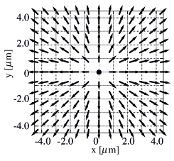
(a) (b) (c)

Figure 1: Properties of the $\langle 0,1,2\rangle$ vortex at $\Omega=0.35$ and $M/N\!=\!0.21$. (a) Density Profile; (b) $l_{x}$ and $l_{y}$; (c) density map of $l_{z}$. The bold line in (a) denotes the total density $n({\bf r})$ and the thin lines show the density of each component $|\psi_{j}|^{2}$.

The axisymmetric $\langle 0,1,2\rangle$ vortex may be parametrized as

$$\left(\begin{array}[]{c}\psi_{1}({\bf r})\\ \psi_{0}({\bf r})\\ \psi_{-1}({\bf r})\end{array}\right)=\sqrt{n(r)}\left(\begin{array}[]{c}\cos^{2}{\beta\over 2}\\ \sqrt{2}e^{i\phi}\sin{\beta\over 2}\cos{\beta\over 2}\\ e^{2i\phi}\sin^{2}{\beta\over 2}\end{array}\right)$$ (50)

where the bending angle $\beta(r)$ runs over $0\leq\beta(r)\leq\pi$ and $\phi$ signifies the polar angle in polar coordinates. The spin direction is denoted by the $l$-vector and is given as $\mbox{\boldmath$l$}(r)={\hat{z}}\cos\beta+\sin\beta(\cos\phi{\hat{x}}+\sin\phi{\hat{y}})$ where $\beta$ varies from $\beta(0)=0$ to $\beta(R)=\frac{\pi}{2}\;(=\pi)$ for MH (Anderson-Toulouse (AT)) ($R$ is the outer boundary of the cloud). Thus the spin moment is flared out to the radial direction and at the circumference it points outward for MH and downwards for AT (for schematic $l$-vector structure, see Fig.18 in Ref.salomaa ).

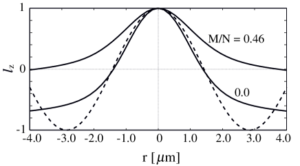
Figure 2: Spatial dependence of the $l_{z}$-component along the radial direction at M/N=0, 0.46, and $\Omega=0.37$. The dashed line shows cos$\beta(r)$ with the bending angle $\beta(r)=\pi r/R$ ($R=2.85\mu m$) for the AT vortex.

In Fig.2 we show the spatial dependence of the $l_{z}$-component along the radial direction, namely, the spatial dependence of the bending angle $\beta(r)$ for the MH vortex. As the magnetization $M$ decreases, the local magnetization in the condensate surface changes from positive to negative passing through zero. It means that the $l$-vector in this vortex flares out radially to orient almost horizontally $\beta(r=R)={\pi\over 2}$ for $M/N\sim 0.5$ and to point downward for $\beta(r=R)=\pi$ for $M/N\sim 0$. The former (latter) corresponds literally to the Mermin-Ho (Anderson-Toulouse) vortex. This is simply because as $M$ decreases, the spin-down component $\psi_{-1}$ with $w=2$ increases in the outer region. Thus we can control these MH and AT vortices by merely changing the total magnetization.

As pointed out in the previous papermizushima , however, the situation is completely different from the case of superfluid ³He-A where the stability of the MH vortex is due to the constraint that the $l$-vector be perpendicular to the vessel wallsalomaa . These vortex configurations in ferromagnetic BEC are created naturally under the condition of a given total number and magnetization, both of which are well controlled in a harmonic trap experiment.

In comparison with the $\langle 0,1,2\rangle$ vortex, the spin textures of other vortex configurations, such as the $\langle 1,\times,0\rangle$ and $\langle 1,0,-1\rangle$ vortices, have a different natureisoshima1 . In $\langle 1,\times,0\rangle$ vortex, the spin moment is suddenly reversed near the vortex core of $\psi_{1}$ component because of the absence of $\psi_{0}$ component. In $\langle 1,0,-1\rangle$ vortex it can vary continuously around the vortex core. In this configuration, however, since the condensate at the center of the trap consists only of the polar stateho , the spin texture has a singularity. Thus only $\langle 0,1,2\rangle$ vortex can have a non-singular and continuous spin texture under slow rotation.

Figure 3: Density profiles of the $\langle 0,1,2\rangle$ vortex in an antiferromagnetic interaction of $g_{s}/g_{n}=0.005$ (on the left) and the non-magnetic interaction of $g_{s}/g_{n}=0$ (on the right) situation.

It is easy to calculate the total angular momentum $L_{z}$ of the axisymmetric vortices; by using the total particle number and the total magnetization, it is simply written as

$$\frac{L_{z}}{\hbar N}=w_{0}+w^{\prime}\frac{M}{N},$$ (51)

where the total magnetization is written as $M=\int d{\bf r}n({\bf r})\hat{l}_{z}$ and we have introduced $w_{j}-w_{0}=jw^{\prime}$. Thus the spin textures with a net spin polarization carry the angular momentum, i.e. the superflow. For $\langle 0,1,2\rangle$ vortex, $\frac{L_{z}}{\hbar N}=1-\frac{M}{N}$. This simple formula has the following physical meaning. (i)At $M\!=\!N$, $L_{z}\!=\!0$ because $\psi_{1}$ has no winding. (ii)At ${M\over N}\!=\!{1\over 2}$, ${L_{z}\over\hbar N}$ is exactly equal to $\hbar/2$, corresponding to the MH vortex.

In the $\langle 0,1,2\rangle$ state with the higher winding, the non-winding component $\psi_{1}$ works as a “pinning potential” for the remaining $\psi_{0}$ and $\psi_{-1}$, thereby making the state stable in the lower rotation drive. In particular, $\psi_{-1}$ with $w_{-1}\!=\!2$ is stabilized by the presence of the $\psi_{1}$ due to the ferromagnetic interaction. For a very small antiferromagnetic interaction ($g_{s}=0.005g_{n}$) and non-magnetic case ($g_{s}/g_{n}\!=\!0$), the vortex with the $w_{-1}\!=\!2$ becomes unstable and splits into a couple of $w_{-1}\!=\!1$ vortices (see Fig.3). This configuration is equivalent to the vortex found by Yip (phase IV in Ref.yip ) and is always unstable for the large $g_{s}/g_{n}$ ($>0$).

III.2 Non-Axisymmetric vortex

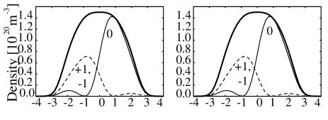
(a)

(b)

Figure 4: Density profiles in the $\langle 1,1,1\rangle$ split-(I) (on the left) and split-(II) vortex (on the right) at $\Omega=0.35$ and $M/N=0$: (a) Non-magnetic interaction case ($g_{s}/g_{n}=0.0$) and (b) $g_{s}=0.4g_{n}$. The bold line show the total density $n({\bf r})$ and the thin and dashed lines present the density profiles of the internal structures, respectively.

To investigate the possibility of non-axisymmetric vortices, let us first recapitulate the axisymmetric $\langle 1,1,1\rangle$ vortex. In the axisymmetric case, the total density of the $\langle 1,1,1\rangle$ vortex is equivalent to the one in scalar BEC, having the singularity at the center of the trap where the potential energy is minimum. The axisymmetric singular $\langle 1,1,1\rangle$ vortex is always unstable even in the higher rotationisoshima2 . However, by displacing the vortex cores of each component from the center of the trap, the $\langle 1,1,1\rangle$ vortex can be stable as a non-axisymmetric non-singular type in the lower rotation frequency. This works favorably to gain more condensation energy at the center of the trap. A similar situation is seen near the $\Omega_{c2}$ in the homogeneous system, where the singular vortex lattice, called the Abrikosov lattices, is never favored in the entire antiferromagnetic regionkita .

For the antiferromagnetic case, $\psi_{1}$ and $\psi_{-1}$ overlap to minimize the spin-dependent energy $E_{s}({\bf r})$. In Fig.4, we show the density profiles and $g_{s}$-dependence of two different $\langle 1,1,1\rangle$ vortices. In the non-magnetic limit ($g_{s}/g_{n}\!=\!0$), the two states are completely equivalent. As the spin interaction $g_{s}/g_{n}$ increases, striking differences grow between the two states. For $g_{s}/g_{n}\!\sim\!0.4$, the vortex cores of the state presented in the left of Fig.4 (b) (the split-(I) state) collapse and the amplitude of each order parameter cannot recover near the vortex cores, i.e. this state behaves like the phase separation in $x$-$y$ plane. In contrast, the state shown in the right of Fig.4 (b) (the split-(II) state) forms the regular cores. As a result, the split-(II) state is energetically favorable over the split-(I) state for the antiferromagnetic situation. In very small spin interaction range ($g_{s}\sim 0.02g_{n}$), which is a realistic parameter, however, the split-(I) state can be favored over the split-(II), though the energies of two states are very close to each other.

(a)
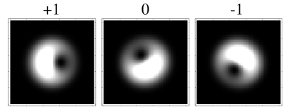
(b)
(c)

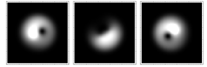
Figure 5: Density profiles of each component $|\psi_{1}({\bf r})|^{2}$, $|\psi_{0}({\bf r})|^{2}$, and $|\psi_{-1}({\bf r})|^{2}$ in $\langle 1,1,1\rangle$ triangle vortex at $\Omega=0.35$ and $M/N=0$: (a) Non-magnetic interaction case ($g_{s}/g_{n}=0.0$), (b) $g_{s}=0.02g_{n}$, and (c) $g_{s}=0.2g_{n}$. The total density profile almost agrees with that in the vortex-free state, i.e. the non-singular type.

A third vortex configuration is displayed in Fig.5 where vortex cores of each component are displaced to form a triangle. In the non-magnetic limit, the three components are completely equivalent and the three singularities form a regular triangle. As the spin interaction $g_{s}$ increases, the $\psi_{1}$ and $\psi_{-1}$ components overlap locally because of the antiferromagnetic interaction and this vortex configuration starts to deform from a regular triangle shape. For larger spin interactions ($g_{s}>0.4$), this vortex becomes unstable due to the overlap between $\psi_{1}$ and $\psi_{-1}$ components.

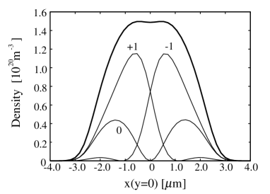
(a)
(b) (c)

Figure 6: (a)Density profile of the condensates, (b)the $l_{x}$ and $l_{y}$ and (c)the density map of $l_{z}$ for the non-axis-symmetric $\langle 1,1,1\rangle$ vortex in $\Omega=0.35$ and M/N=0.0. The bold line is the total density $n({\bf r})$ and the thin lines show the density of each component $|\psi_{j}|^{2}$.

Figure 6 (a) shows the density profiles of a non-axisymmetric non-singular $\langle 1,1,1\rangle$ vortex for the ferromagnetic case. Two singularities of $\psi_{1}$ and $\psi_{-1}$ are displaced from the center. The $\psi_{0}$ component with the singularity at the center of the trap plays the role to prevent the phase separation favored in the ferromagnetic spin interaction. The spin texture in this state is displayed in Figs.6 (b) and (c) where the spin moments flip at the center of the trap.

In comparison with axisymmetric types, these non-axisymmetric vortices have the advantage that they can easily adjust themselves for a change in $\Omega$. As $\Omega$ increases, the two or three separate singularities adjust their mutual distance from the center and change the value of $L_{z}$ to gain the energy from the term $-\Omega L_{z}$. In this sense, the non-axisymmetric vortices are flexible against a change in $\Omega$ compared with the axisymmetric ones.

IV phase diagram

The phase diagrams are shown in a plane of the external rotation and the total magnetization by comparing the energies of various vortex configurations:

$$E=\int d{\bf r}\left[\sum_{i}E_{i}({\bf r})+E_{s}({\bf r})\right]-\Omega L_{z}.$$ (52)

It is noted that the region $\Omega\!<\!0.38$ considered here corresponds to the single vortex region in the scalar BEC caseisoshima3 . Thus, the present single-vortex consideration may also be justified for $\Omega<0.38$.

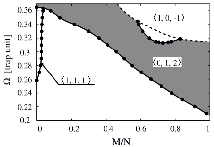
(a) (b)

Figure 7: Phase diagram for (a)the ferromagnetic state ($g_{s}=-0.02g_{n}$) and (b)the antiferromagnetic case ($g_{s}=0.02g_{n}$). The dashed line in (a) denotes the boundary where the lowest quasiparticle energy of the $\langle 0,1,2\rangle$ vortex becomes negativemizushima .

The resulting phase diagram is displayed in Fig.7 for (a) the ferromagnetic case and (b) the antiferromagnetic case. For the ferromagnetic case, a large area of the $\Omega-M$ plane is occupied by the $\langle 0,1,2\rangle$ vortex, including MH and AT. The non-axisymmetric $\langle 1,1,1\rangle$ vortex and the $\langle 1,0,-1\rangle$ vortex are stabilized near $M\!=\!0$ and $M\!=\!N$, respectively. We find a large empty area in the intermediate $M/N$ region where neither single-vortex nor vortex-free states are stabilized at all because the phase separation in the ferromagnetic case prevents forming a uniform mixture of the three components even when the circulation is absent in the vortex-free state.

In the phase diagram for the antiferromagnetic case, in contrast, everywhere is occupied by a stable phase. This result is consistent with Fig.2(a) of Ref.isoshima2 over a wide range, except for the presence of two non-axisymmetric types near $M\sim 0$, i.e. $\langle 1,1,1\rangle$ split-(I) and triangle vortex. The $\langle 1,1,1\rangle$ triangle vortex is energetically indistinguishable from the phase-I vortex obtained by Yipyip . The phase-IV vortex given in Fig,3 of Ref.yip is found unstable for $g_{s}\!=\!0.02g_{n}$ and does not appear in this phase diagram.

(a)

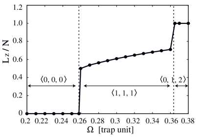
(b)

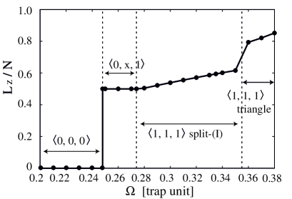
Figure 8: $\Omega$-dependence of the angular momentum $L_{z}/N$ at $M/N=0$: (a) the ferromagnetic case ($g_{s}\!=\!-0.02g_{n}$) and (b) the antiferromagnetic case ($g_{s}\!=\!0.02g_{n}$).

It is found for both cases that the stabilities of the non-axisymmetric vortices are restricted in a narrow region. On the other hand, the axisymmetric vortices are stable in a large area. As discussed in Section III, since finite density of a component at the vortex cores of the others supports its stability, the non-axisymmetric vortex becomes unstable in increasing $M$ where the number of $\psi_{1}$ grows while the others shrink.

Figure 8 shows the $\Omega$-dependence of the angular momentum at $M=0$ for the two cases. For axisymmetric types, as shown in Eq.(51), the angular momentum of the system $L_{z}$ is fixed for a given $M$. Thus there is the need of changing the winding combinations $\langle w_{1},w_{0},w_{-1}\rangle$ so as to increase $L_{z}$, which means that the axisymmetric vortices do not have the adaptability for changes in $\Omega$.

V Discussion

The phase-separated state with $w\!=\!0$ is expected to be stable in a large empty region of Fig.7 (a). In this state, $\psi_{1}$ and $\psi_{-1}$ components phase-separate along $z$-direction due to the ferromagnetic interaction. Namely, an arbitrary $x$-$y$ cross-section consists of only $\psi_{1}$ or $\psi_{-1}$ component, and the spin-polarized state with $M/N\!=\!\pm 1$ is piled up along the z-direction. Neglecting the contribution from the boundary layer associated with the phase separation, we can estimate that the energy of this phase-separated state with $w\!=\!0$ and $w\!=\!1$ is equal to the energy of the scalar BEC with $w\!=\!0$ and $w\!=\!1$, respectively.

We compare in Fig.9 (a) the free energies of the $\langle 0,1,2\rangle$ vortex state and the phase-separated state. As shown in Fig.9 (a), the $\langle 0,1,2\rangle$ vortex with the three components is energetically favored over the phase-separated state, where the energy of the phase-separated state is given by the energy of the $\langle 0,1,2\rangle$ vortex at $M/N\!=\!1$, i.e. the scalar BEC with $w\!=\!0$. Thus, the composite state of the three components, such as the MH vortex, becomes “locally” stable under a rotation drive while the composite state may have “global” stability. It is possible to perform a similar discussion for the phase-separated state in higher rotation. The result of Fig.9 (b) shows that the $\langle 1,0,-1\rangle$ vortex is favored over the phase-separated state with the winding, whose total density corresponds to the conventional singular vortex in the scalar BEC.

(a)

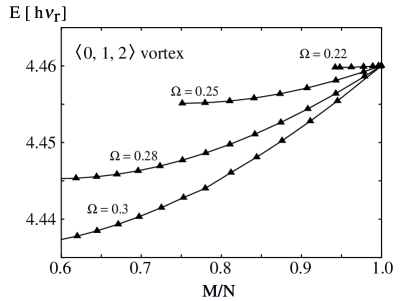
(b)

Figure 9: The $M$-dependence of the energy for the ferromagnetic case: (a)the $\langle 0,1,2\rangle$ and (b)the $\langle 1,0,-1\rangle$ vortices. The energies of the phase-separated states with $w\!=\!0$ and $w\!=\!1$ correspond to the energies of the $\langle 0,1,2\rangle$ vortex at $M/N\!=\!1$ and $\langle 1,0,-1\rangle$ vortex at $M/N\!=\!1$, respectively.

VI Conclusion

We have presented possible vortex structures and the vortex phase diagram in the plane of external rotation $\Omega$ and the total magnetization $M/N$ for the both cases of antiferromagnetic ($g_{s}=0.02g_{n}$) and ferromagnetic ($g_{s}=-0.02g_{n}$) interaction. We have investigated the thermodynamic stability of the possible vortex configurations by solving the extended Gross-Pitaevskii equation for the spinor BEC with $F=1$.

For the ferromagnetic case, the stability of the continuous vortex, called the Mermin-Ho and Anderson-Toulouse vortex, is demonstrated, but these topological structures are found never stable under no rotation drive. Furthermore, these vortices can exist in the intermediate process (see Fig.5 in the Ref.isoshima4 ) proposed by Isoshima et al.isoshima4 ; nakahara , i.e. it may be created by making use of spin texture.

We have also discovered a couple of new non-axisymmetric vortices besides the two vortices found by Yipyip for the antiferromagnetic case. The conventional singular vortex is found to be never favored in spinor BEC for both cases. It means that the total density profile is always non-singular and continuous. Therefore, the experimental procedure to image the magnetic patterns for each vortex configuration will be required as a special technique to identify these vortices.

- (1) M.H. Anderson, J.R. Ensher, M.R. Matthews, C.E. Wieman and E. Cornell, Science 269, 198 (1995).
- (2) C.C. Bradley, C.A. Sackett, J.J. Tollett and R.G. Hulet, Phys. Rev. Lett. 75, 1687 (1995).
- (3) K.B. Davis, M.-O. Mewes, M.R. Andrews, N.J. van Druten, D.S. Durfee, D.M. Kurn and W. Ketterle, Phys. Rev. Lett. 75 3969 (1995).
- (4) M.R. Matthews, B.P.Anderson, P.C. Haljan, D.S. Hall, C.E. Wieman and E.A. Cornell, Phys. Rev. Lett. 83, 2498 (1999).
- (5) K.W. Madison, F. Chevy, W. Wohlleben and J. Dalibard, Phys. Rev. Lett, 84, 806 (2000).
- (6) J.R. Abo-Shaeer, C, Raman, J.M. Vogels and W. Ketterle, Science 292, 476 (2001).
- (7) P.C. Haljan, I. Coddington, P. Engels and E.A. Cornell, Phys. Rev. Lett. 87, 210403 (2001).
- (8) E. Hodby, G. Heckenblaikner, S.A. Hopkins, O.M. Maragó and C.J. Foot, Phys. Rev. Lett. 88, 010405 (2001).
- (9) A.E. Leanhardt, A. Görlitz, A.P. Chikkatur, D. Kielpinski, Y. Shin, D.E. Pritchard, and W. Ketterle, cond-mat/0206303.
- (10) M. Barrett, J. Sauer and M.S. Chapman, Phys. Rev. Lett. 87, 010404 (2001).
- (11) J. Stenger, S. Inouye, D.M. Stamper-Kurn, H.-J. Miesner, A.P. Chikkatur and W. Ketterle, Nature 369, 345 (1998).
- (12) N.N. Klausen, J.L. Bohn and C.H.Greene, Phys. Rev. A 64, 053602 (2001).
- (13) See for review, F. Dalfovo, S. Giorgini, L.P. Pitaevskii, and S. Stringari, Rev. Mod. Phys. 71, 463 (1999).
- (14) T. Ohmi and K. Machida, J. Phys. Soc. Jpn. 67, 1822 (1998).
- (15) T.-L. Ho, Phys. Rev. Lett. 81, 742 (1998).
- (16) R. Rajaraman, Solitons and Instanton (North-Holland, Amsterdam, 1982); N.D. Mermin, Rev. Mod. Phys. 51, 591 (1979).
- (17) A.J. Leggett, Rev. Mod. Phys. 73, 307 (2001).
- (18) N.D. Mermin and T.-L. Ho, Phys. Rev. Lett. 36, 594 (1976).
- (19) P.W. Anderson and G. Toulouse, Phys. Rev. Lett. 38, 508 (1977).
- (20) U. Al Khawaja and H.T.C. Stoof, Nature 411, 918 (2001), and Phys. Rev. A 64, 043612 (2001).
- (21) T. Mizushima, K. Machida, and T. Kita, Phys. Rev. Lett. 89, 030401 (2002).
- (22) K.-P. Marzlin, W. Zhang and B.C. Sanders, Phys. Rev. A 62, 013602 (2000).
- (23) Th. Busch and J.R. Anglin, Phys. Rev. A 60, R2669 (1999).
- (24) S. Tuchiya and S. Kurihara, J. Phys. Soc. Jpn. 70, 1182 (2001).
- (25) J.-P. Martikainen, A. Collin, and K.-A. Suominen, Phys. Rev. Lett. 88, 090404 (2002).
- (26) S.-K. Yip, Phys. Rev. Lett. 83, 4677 (1999).
- (27) T. Isoshima, K. Machida and T. Ohmi, J. Phys. Soc. Jpn. 70, 1604 (2001).
- (28) T. Isoshima and K. Machida, Phys. Rev. A (2002), cond-mat/0201507.
- (29) Y. Castin and R. Dum, Eur. Phys. J. D 7, 399 (1999).
- (30) J.J. García-Ripoll and V.M. Pérez-García, Phys. Rev. A 63, 041603 (2001).
- (31) A. Aftalion and Q. Du, Phys. Rev. A 64, 063603 (2001).
- (32) D.L. Feder and C.W. Clark, Phys. Rev. Lett. 87, 190401 (2001).
- (33) M.M. Salomaa and G.E. Volovik, Rev. Mod. Phys. 59, 533 (1987).
- (34) T. Kita, T. Mizushima, and K. Machida, cond-mat/0204025.
- (35) T. Isoshima and K. Machida, Phys. Rev. A 60, 3313 (1999).
- (36) M. Nakahara, T. Isoshima, K. Machida, S. Ogawa and T. Ohmi, Physica B 284-288, 17 (2000).
- (37) T. Isoshima, M. Nakahara, T. Ohmi and K. Machida, Phys. Rev. A 61, 063610 (2000)