Theory of Two-Dimensional Josephson Arrays in a Resonant Cavity

Abstract

We consider the dynamics of a two-dimensional array of underdamped Josephson junctions placed in a single-mode resonant cavity. Starting from a well-defined model Hamiltonian, which includes the effects of driving current and dissipative coupling to a heat bath, we write down the Heisenberg equations of motion for the variables of the Josephson junction and the cavity mode, extending our previous one-dimensional model. In the limit of large numbers of photons, these equations can be expressed as coupled differential equations and can be solved numerically. The numerical results show many features similar to experiment. These include (i) self-induced resonant steps (SIRS’s) at voltages $V=n\hbar\Omega/(2e)$, where $\Omega$ is the cavity frequency, and $n$ is generally an integer; (ii) a threshold number $N_{c}$ of active rows of junctions above which the array is coherent; and (iii) a time-averaged cavity energy which is quadratic in the number of active junctions, when the array is above threshold. Some differences between the observed and calculated threshold behavior are also observed in the simulations and discussed. In two dimensions, we find a conspicuous polarization effect: if the cavity mode is polarized perpendicular to the direction of current injection in a square array, it does not couple to the array and there is no power radiated into the cavity. We speculate that the perpendicular polarization would couple to the array, in the presence of magnetic-field-induced frustration. Finally, when the array is biased on a SIRS, then, for given junction parameters, the power radiated into the array is found to vary as the square of the number of active junctions, consistent with expectations for a coherent radiation. For a given step, a two-dimensional array radiates much more energy into the cavity than does a one-dimensional array.

I Introduction

The properties of arrays of Josephson junctions have been of great interest for nearly twenty years.review Such arrays are excellent model systems in which to study such phenomena as phase transitions and quantum coherence in two dimensions. For example, if only the Josephson coupling energy is considered, the Hamiltonian of a two-dimensional (2D) array of Josephson junctions is formally identical to that of a 2D XY model [see, e. g. Ref. chaikin, ]. Arrays sometimes appear to mimic behavior seen in nominally homogeneous materials, such as high-$T_{c}$ superconductors, which often behave as if they are composed of distinct superconducting regions linked together by Josephson coupling.tinkham Finally, the arrays are of potentially practical interest: they may be useful, for example, as sources of coherent microwave radiation if the individual junctions can be caused to oscillate in phase in a stable manner.

Recently, our ability to achieve this kind of stable oscillation, and coherent microwave radiation, was significantly advanced by a series of experiments by Barbara and collaborators.barbara ; barbara02 ; asc2000 ; vasilic02 ; vasilic These workers placed two-dimensional underdamped Josephson arrays in a geometry which allowed them to be coupled to a resonant microwave cavity. The presence of the cavity caused the junctions to couple together far more efficiently than in its absence. As a result, the power radiated into the cavity has been found to be as much as 30% of the d. c. power injected into the array, far higher than the efficiency achieved in previous experiments. Even more surprising, this efficiency is achieved in underdamped arrays, which according to conventional wisdom should be especially difficult to synchronize, since each such junction exhibits bistability and hysteresis as a function of the external control parameters. These experiments have stimulated many theoretical attempts to explain them.filatrella ; filatrella2 ; almaas ; almaas02_2

In our previous work, we have presented a simple one-dimensional (1D) model which seems to account for many features of the observed cavity-induced coherence.almaas ; almaas02_2 Despite the geometrical differences, the 1D model does a surprisingly good job of capturing the physics of the experiments. However, a truly realistic test requires that the model be extended to a geometry closer to the experimental one. In this paper, therefore, we present the necessary extension to 2D. Our results give significant insight into why the 1D model works so well. In addition, they provide some clues about how one might understand experimental features which are still unexplained in either the 1D or the 2D models.

The remainder of this paper is organized as follows. In the next section, we describe our model Hamiltonian for a 2D current-driven, underdamped Josephson junction array in a resonant cavity which supports a single mode. This Hamiltonian is a straightforward extension of that used in our previous work to describe 1D arrays. In Section III, using this Hamiltonian, we write out the Heisenberg equations of motion for the junction variables and for the photon creation and annihilation operators for the cavity mode. We incorporate resistive dissipation in the junctions in a standard way, by coupling the gauge-invariant phase differences across each junction to its own set of harmonic oscillator variables whose spectral density is chosen to produce Ohmic dissipation. In the limit of large numbers of photons, we obtain classical equations of motion for the variables. In Section IV, we present the numerical solutions of this model with an emphasis on features special to 2D, and we also give a comparison between the 2D and previous 1D results. A concluding discussion and comparison with experiment follows in Section V.

II Model Hamiltonian

We will consider a 2D array of $N\times M$ superconducting grains placed in a resonant cavity, which we assume supports only a single photon mode of frequency $\Omega$. The array is thus made up of $(N-1)(M-1)$ square plaquettes. There are a total of $N_{x}\times N_{y}$ horizontal junctions, where $N_{x}=N-1$ and $N_{y}=M$. A current $I$ is fed into each of the $M$ grains on the left edge of the array, and extracted from each of the $M$ grains on the right edge. Thus, the current is inject in the $x$ direction, with no external current injected in the $y$ direction. A sketch of this geometry is shown in Fig. 1. We also introduce the terminology that a “row” of junctions, in this configuration, refers to a group of $N_{y}$ junctions, all with left-hand end having the same $x$ coordinate, and all being parallel to the bias current. One such row is indicated by the dashed lines in Fig. 1.

In contrast to our previous work,almaas02_2 we will write the equations of motion for the grain variables (phases and charges) rather than junction variables, since in 2D, the junction variables cannot be treated as all independent (there are twice as many junctions as grains).

We express our Hamiltonian in a form analogous to that of Ref. almaas02_2, :

$$H=H_{photon}+H_{J}+H_{C}+H_{curr}+H_{diss}.$$ (1)

Here $H_{photon}$ is the energy of the cavity mode, expressed as

$$H_{photon}=\hbar\Omega\left(a^{\dagger}a+\frac{1}{2}\right),$$ (2)

where $a^{\dagger}$ and $a$ as the usual photon creation and annihilation operators. $H_{J}$ is the Josephson coupling energy, and is assumed to take the form

$$H_{J}=-\sum_{\langle ij\rangle}E^{J}_{ij}\cos(\gamma_{ij}),$$ (3)

where $E^{J}_{ij}$ is the Josephson energy of the (ij)^th junction, and $\gamma_{ij}$ is the gauge-invariant phase difference across that junction (defined more precisely below). $E^{J}_{ij}$ is related to $I^{c}_{ij}$, the critical current of the (ij)^th junction, by $E^{J}_{ij}=\hbar I_{ij}^{c}/q$, where $q=2|e|$ is the Cooper pair charge. $H_{C}$ is the capacitive energy of the array, which we write in a rather general form as

$$H_{C}=\frac{1}{2}\sum_{ij}q^{2}(C^{-1})_{ij}n_{i}n_{j},$$ (4)

where $C^{-1}$ is the inverse capacitance matrix, $n_{i}$ is the number of Cooper pairs on the $i^{th}$ grain, and $q=2e$ is the charge of a Cooper pair (we take $e>0$). Note that in Ref. almaas02_2, , the variable $n_{i}$ was used to denote the difference between the numbers of Cooper pairs on the two grains comprising junction $i$.

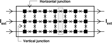
Figure 1: Sketch of the array geometry considered in our model. There are $(M\times N)$ superconducting islands (black squares), making ${[}(M-1)\times N+(N-1)\times M{]}$ Josephson junctions (crosses). An external current $I^{ext}$ is injected into each junction at one end of the array and extracted from each junction at the other end. The array is placed in an electromagnetic cavity which supports a single resonant photon mode of frequency $\Omega$. We have indicated by dashes a group of junctions which we denote a “row.” Such a row is perpendicular to the current bias and is comprised of horizontal junctions.

As in 1D, the gauge-invariant phase difference, $\gamma_{ij}$, is the term which leads to coupling between the Josephson junctions and the cavity. We write it as

$$\gamma_{ij}=\phi_{i}-\phi_{j}-[(2\pi)/\Phi_{0}]\int_{ij}{\bf A}\cdot{\bf ds}\equiv~{}\phi_{i}-\phi_{j}-A_{ij},$$ (5)

where $\phi_{i}$ is the gauge-dependent phase of the superconducting order parameter on grain $i$, and ${\bf A}$ is the vector potential, which (in Gaussian units) takes the formslater ; yariv

$${\bf A}({\bf x},t)=\sqrt{(hc^{2})/(\Omega)}\left(a(t)+a^{\dagger}(t)\right){\bf E}({\bf x}),$$ (6)

where ${\bf E}({\bf x})$ is a vector proportional to the local electric field of the mode, normalized such that $\int_{V}d^{3}x|{\bf E}({\bf x})|^{2}=1$, and $V$ is the cavity volume. The line integral is taken across the (ij)^th junction.

Given this representation for ${\bf A}$, the phase factor $A_{ij}$ can be written

$$A_{ij}=g_{ij}(a+a^{\dagger}),$$ (7)

where $g_{ij}$ takes the form

$$g_{ij}=\sqrt{\frac{\hbar c^{2}}{\Omega}\frac{(2\pi)^{3}}{V\Phi_{0}^{2}}}\int_{ij}{\bf E}\cdot{\bf ds}$$ (8)

Clearly, $g_{ij}$ is an effective coupling constant describing the interaction between the (ij)^th junction and the cavity.

We include a driving current and dissipation in a manner similar to that of Ref. almaas02_2, . The driving current is included via a “washboard potential,” $H_{curr}$, of the form

$$H_{curr}=-\frac{\hbar I^{ext}}{q}\sum_{\langle ij\rangle\|\bf{\hat{x}}}\gamma_{ij},$$ (9)

where $I$ is the driving current injected in the $x$ direction into each grain on the left edge (and extracted from the right edge), and the sum runs over only those bonds in the $x$ direction (each such bond is counted once). To introduce dissipation, each gauge-invariant phase difference, $\gamma_{ij}$, is coupled to a separate collection of harmonic oscillators with a suitable spectral density.ambeg ; caldeira81 ; leggett ; chakra Thus, the dissipative term in the Hamiltonian is

$$H_{diss}=\sum_{\langle ij\rangle}H_{ij}^{diss},$$ (10)

where the sum runs over distinct bonds $\langle ij\rangle$, and

$$H_{ij}^{diss}~{}=~{}\sum_{\alpha}\Bigg{[}f_{\alpha,ij}~{}\gamma_{ij}~{}u_{\alpha,ij}+\frac{(p_{\alpha,ij})^{2}}{2m_{\alpha,ij}}+$$

$$\frac{1}{2}m_{\alpha,ij}~{}(\omega_{\alpha,ij})^{2}~{}(u_{\alpha,ij})^{2}+\frac{(f_{\alpha,ij})^{2}}{2~{}m_{\alpha,ij}~{}(\omega_{\alpha,ij})^{2}}~{}(\gamma_{ij})^{2}\Bigg{]}.$$ (11)

The variables $u_{\alpha,ij}$ and $p_{\alpha,ij}$, describing the $\alpha^{th}$ oscillator in the (ij)^th junction, are canonically conjugate, and $m_{\alpha,ij}$ and $\omega_{\alpha,ij}$ are the mass and frequency of that oscillator. By choosing the spectral density, $J_{ij}(\omega)$, to be linear in $|\omega|$, we assure that the dissipation in the junction is ohmic.caldeira81 ; leggett We write such a linear spectral density as

$$J_{ij}(\omega)=\frac{\hbar}{2\pi}~{}\alpha_{ij}~{}|\omega|~{}\Theta(\omega_{c}-\omega),$$ (12)

where $\omega_{c}$ is a high-frequency cutoff (at which the assumption of ohmic dissipation begins to break down), $\Theta(\omega_{c}-\omega)$ is the usual step function, and $\alpha_{ij}$ is a dimensionless constant. We write it as $\alpha_{ij}=R_{0}/R_{ij}$, where $R_{0}=h/(4e^{2})$ and $R_{ij}$ is a constant with dimensions of resistance (which proves to be the effective shunt resistance of the junction, as discussed below).

III Equations of motion

To obtain equations of motion, it is convenient to introduce the operators $a=a_{R}+ia_{I}$ and $a^{\dagger}=a_{R}-ia_{I}$. These have the commutation relation $[a_{R},a_{I}]=i/2$, which follows $[a,a^{\dagger}]=1$. In terms of these variables,

$$H_{photon}=\hbar\Omega(a_{R}^{2}+a_{I}^{2}),$$ (13)

and $\gamma_{ij}$ takes the form

$$\gamma_{ij}=\phi_{i}-\phi_{j}-2g_{ij}a_{R}.$$ (14)

The time-dependence of the various operators appearing in the Hamiltonian (1) is now obtained from the Heisenberg equations of motion. These are readily derived from the commutation relations for the various operators in the Hamiltonian (1). Besides the relations already given, the only non-zero commutators are

$${[}n_{j},\phi_{k}{]} = -i\delta_{jk};$$ (15)

$${[}p_{\alpha,ij},u_{\beta,k\ell}{]} = -i\hbar~{}\delta_{\alpha,\beta}~{}\delta_{ij,k\ell},$$ (16)

where the last delta function vanishes unless $(ij)$ and $(k\ell)$ refer to the same junction.

Using all these relations, we find, after a little algebra, the following equations of motion for the operators $\phi_{i}$, $n_{i}$, $a_{R}$, and $a_{I}$:

$$\dot{\phi}_{i} = \frac{q^{2}}{\hbar}\sum_{j}(C^{-1})_{ij}n_{j},$$ (17)

$$\dot{n}_{i} = -\frac{1}{\hbar}\sum_{l}E^{J}_{il}\sin(\phi_{i}-\phi_{l}-2g_{il}a_{R})+\frac{I_{i}^{ext}}{q}-\frac{1}{\hbar}\sum_{l}\sum_{\alpha}\left[u_{\alpha,il}f_{\alpha,il}+\frac{(f_{\alpha,il})^{2}}{m_{\alpha,il}(\omega_{\alpha,il})^{2}}(\phi_{i}-\phi_{l}-2g_{il}a_{R})\right],$$ (18)

$$\dot{a}_{R} = \Omega~{}a_{I},$$ (19)

$$\dot{a}_{I} = -\Omega~{}a_{R}+\sum_{\langle ij\rangle}g_{ij}\frac{E^{J}_{ij}}{\hbar}~{}\sin(\phi_{i}-\phi_{j}-2g_{ij}a_{R})-\frac{I^{ext}}{q}\sum_{\langle ij\rangle\|{\bf\hat{x}}}g_{ij}$$ (20)

$$+\sum_{\langle ij\rangle}\frac{g_{ij}}{\hbar}~{}\sum_{\alpha}\left(f_{\alpha,ij}~{}u_{\alpha,ij}+\frac{(f_{\alpha,ij})^{2}}{m_{\alpha,ij}\omega_{\alpha,ij}^{2}}~{}(\phi_{i}-\phi_{j}-2g_{ij}a_{R})\right).$$

Here, the index $l$ ranges over the nearest-neighbor grains of $i$. In writing these equations, we have assumed that the only external currents $I_{i}^{ext}$ are those along the left and right edges of the array, where they are $\pm I^{ext}$ [cf. Fig. 1]. Eqs. (17)-(20) are equations of motion for the operators $a_{R}$, $a_{I}$, $n_{j}$, and $\phi_{j}$ (or $\gamma_{j}$). In order to make these equations amenable to computation, we will later regard these operators as $c$-numbers, as we did earlier in 1D.almaas02_2 This approximation is expected to be reasonable when there are many photons in the cavity.almaas02_2

The equations of motion for the harmonic oscillator variables can also be written out explicitly. However, since we have no direct interest in these variables, we instead eliminate them in order to incorporate a dissipative term directly into the equations of motion for the other variables. Such a replacement is possible provided that the spectral density of each junction is linear in frequency, as noted above. In that case,ambeg ; caldeira81 ; leggett ; chakra ; almaas02_2 the oscillator variables can be integrated out. The effect of carrying out this procedure is that one should make the replacement

$$\sum_{\alpha}\left(f_{\alpha,ij}~{}u_{\alpha,ij}+\frac{(f_{\alpha,ij})^{2}}{m_{\alpha,ij}\omega_{\alpha,ij}^{2}}~{}\gamma_{ij}\right)\rightarrow\frac{\hbar}{2\pi}\frac{R_{0}}{R_{ij}}~{}\dot{\gamma}_{ij}$$ (21)

wherever this sum appears in the equations of motion. Making the replacement (21) in Eqs. (18) and (20), and simplifying, we obtain the equations of motion for $n_{j}$ and $a_{I}$ with damping:

$$\dot{n}_{i} = -\sum_{j}\frac{E^{J}_{ij}}{\hbar}\sin(\gamma_{ij})+\frac{I^{ext}_{i}}{q}-\sum_{j}\frac{1}{2\pi}\frac{R_{0}}{R_{ij}}\dot{\gamma}_{ij}$$ (22)

$$\dot{a}_{I} = -\Omega~{}a_{R}+\sum_{\langle ij\rangle}g_{ij}\frac{E_{ij}}{\hbar}~{}\sin(\gamma_{ij})-\frac{I^{ext}}{q}\sum_{\langle ij\rangle\|{\bf\hat{x}}}g_{ij}+\sum_{\langle ij\rangle}g_{ij}~{}\frac{R_{0}}{2\pi R_{ij}}\dot{\gamma}_{ij}.$$ (23)

Once, again, the index $j$ is summed only over the nearest-neighbor grains of $i$. Equations (17), (19), (22), and (23) form a closed set of equations which can be solved for the time-dependent functions $\gamma_{i}$, $n_{i}$, $a_{R}$ and $a_{I}$, given the external current and the other parameters of the problem.

It is now convenient to express these equations of motion in terms of suitable scaled variables. We therefore introduce a dimensionless time $\tau=tqRI^{c}/\hbar=\omega_{\tau}t$, where $R$ and $I^{c}$ are suitable averages over $R_{ij}$ and $I^{c}_{ij}$. We also define the other scaled variables

$$\tilde{R}_{ij} = \frac{R_{ij}}{R},$$ (24)

$$\tilde{\Omega} = \frac{\Omega}{\omega},$$ (25)

$$\tilde{I} = \frac{I}{I^{c}},$$ (26)

$$\tilde{V}_{i} = \frac{V_{i}}{RI^{c}},$$ (27)

$$\tilde{a}_{R,I} = \sqrt{2\pi\frac{R}{R_{0}}}a_{R,I},$$ (28)

$$\tilde{g}_{ij} = \sqrt{\frac{R_{0}}{2\pi R}}g_{ij},$$ (29)

$$\tilde{C}_{ij} = \omega_{\tau}RC_{ij}.$$ (30)

The last equation involves the capacitance matrix $C_{ij}$. We assume that this takes the form fazio ; kim

$$C_{ij} = \left(C_{d}+z_{i}~{}C_{c}\right)\delta_{ij}$$ (31)

$$-C_{c}\left(\delta_{i,j+{\bf\hat{x}}}+\delta_{i,j-{\bf\hat{x}}}+\delta_{i,j+{\bf\hat{y}}}+\delta_{i,j-{\bf\hat{y}}}\right),$$

i. e., that there is a nonvanishing capacitance only between neighboring grains and between a grain and ground. Here $z_{i}(=4)$ is the number of nearest neighbors of grain $i$, $C_{d}$ and $C_{c}$ are respectively the diagonal (self) and nearest-neighbor capacitances, and ${\bf\hat{x}}$ and ${\bf\hat{y}}$ are unit vectors in the $x$ and $y$ directions. The corresponding Stewart-McCumber parameters are $\beta_{c}=\omega_{\tau}RC_{c}$ and $\beta_{d}=\omega_{\tau}RC_{d}$.

In Eq. (27), we introduced the potential $V_{i}$ on site $i$, which is expressed through the number variables $n_{j}$ as

$$V_{i}~{}=~{}q\sum_{j}(C^{-1})_{ij}n_{j}.$$ (32)

The integral of the electric field across junction $(ij)$ is written in terms of the $V_{i}$’s as

$$V_{ij}~{}=~{}V_{i}-V_{j}-2\tilde{g}_{ij}\Omega a_{I}.$$ (33)

Carrying out these variable changes, we find, after some algebra, that the equations of motion can be expressed in the following dimensionless form:

$$\frac{d}{d\tau}~{}\phi_{i} = \tilde{V}_{i},$$ (34)

$$\frac{d}{d\tau}~{}\tilde{V}_{i} = \sum_{j}(\tilde{C}^{-1})_{ij}\Bigg{[}\tilde{I}_{j}^{ext}-\sum_{l}\Bigg{(}\tilde{I}_{jl}^{c}\sin(\phi_{j}-\phi_{l}-2\tilde{g}_{jl}a_{R})+\frac{1}{\tilde{R}_{jl}}(\tilde{V}_{i}-\tilde{V}_{l}-2\tilde{g}_{il}\tilde{\Omega}\tilde{a}_{I})\Bigg{)}\Bigg{]},$$ (35)

$$\frac{d}{d\tau}~{}\tilde{a}_{R} = \tilde{\Omega}\tilde{a}_{I},$$ (36)

$$\frac{d}{d\tau}~{}\tilde{a}_{I} = -\tilde{\Omega}\tilde{a}_{R}+\sum_{\langle ij\rangle}\tilde{g}_{ij}\Bigg{[}\tilde{I}_{ij}^{c}\sin(\phi_{i}\!-\!\phi_{j}\!-\!2\tilde{g}_{ij}\tilde{a}_{R})+\frac{1}{\tilde{R}_{ij}}(\tilde{V}_{i}-\tilde{V}_{j}-2\tilde{\Omega}\tilde{g}_{ij}\tilde{a}_{I})\Bigg{]}-\tilde{I}^{ext}\!\!\!\sum_{\langle ij\rangle\|{\bf\hat{x}}}\!\!\tilde{g}_{ij}.$$ (37)

These equations are readily generalized to treat external currents with non-zero components in both the $x$ and the $y$ directions, and to geometries other than lattices with square primitive cells.

IV Numerical results

We solve Eqs. (34) – (37) numerically, by implementing the adaptive Bulrisch-Stoer method,numrec as described further in Ref. almaas02_2, . For simplicity, we assume that the coupling constants $\tilde{g}_{ij}$ have only two possible values, $\tilde{g}_{x}$ and $\tilde{g}_{y}$, corresponding to junctions in the $x$ and $y$ direction respectively.note1 This assumption should be reasonable if two conditions are satisfied: (i) there is not much disorder in the characteristics of the individual junctions; and (ii) the wavelength of the resonant mode is large compared to the array dimensions. Although assumption (ii) is not obviously satisfied for the experimental arrays, the model may still be reasonable in certain array/cavity geometries, as discussed further below.

In the presence of a vector potential, it is customary to define a frustration $f_{\mu}(\tau)$ for the $\mu^{th}$ plaquette by the relationteitel

$$f_{\mu}(\tau) = \frac{1}{2\pi}\!\sum_{plaquette}\!\!\!\!A_{ij}~{}=~{}\frac{\tilde{a}_{R}(\tau)}{\pi}\!\!\sum_{plaquette}\!\!\!\!\tilde{g}_{ij},$$ (38)

where the sum runs over bonds in the $\mu^{th}$ plaquette. For a general position-dependent $\tilde{g}_{ij}$, $f_{\mu}(\tau)\neq 0$, but if $\tilde{g}_{x}$ and $\tilde{g}_{y}$ are both position-independent, then $f_{\mu}(\tau)=0$. The possibility of having distinct coupling constants $\tilde{g}_{x}$ and $\tilde{g}_{y}$ along $x$ and $y$ bonds arises from differences in possible polarizations of the resonant mode, and leads to effects which cannot be captured in a 1D model, as discussed below.

Before discussing our numerical results, we briefly summarize one well-known feature of underdamped Josephson arrays in the absence of coupling to a resonant cavity. At certain applied currents, the individual junctions in such an array are bistable - that is, they can be placed in an “active” (resistive) or an “inactive” (superconducting) state, by a careful choice of initial conditions. For an applied current in the $x$ direction, when a single horizontal junction is chosen to be in the active state, it is found that all the other horizontal junctions in the same “row” (cf. Fig. 1) also go active, provided that there is at least a little disorder in the junction critical currents [cf., e. g., Refs. wenbin1, and wenbin92, ]. In our simulations for 2D arrays coupled to a resonant cavity, we observe this same phenomenon, as discussed below.

IV.1 Horizontal coupling

We first consider the case $\tilde{g}_{x}\neq 0$, $\tilde{g}_{y}=0$, with driving current parallel to the $x$ axis. In Fig. 2, we show a series of current-voltage (IV) characteristics for this case. We consider an array of $10\times 4$ grains, with capacitances $\beta_{c}=20$ and $\beta_{d}=0.05$, $\tilde{g}_{x}=0.012$, and $\tilde{\Omega}=0.41$. The critical current through the (ij)^th junction is $\tilde{I}_{ij}^{c}=1+\Delta_{ij}$ where the disorder $\Delta_{ij}$ is randomly selected with uniform probability from $[-\Delta,\Delta]$. In this plot, $\Delta=0.05$. The product $\tilde{I}_{ij}^{c}\tilde{R}_{ij}$ is assumed to be the same for all junctions, in accordance with the Ambegaokar-Baratoff expression.ambegaokar In addition, $\beta_{d}$ and $\beta_{c}$ are assumed to be the same for all junctions. The calculated IV’s are shown as a series of points. The directions of the arrows indicate whether the curves were obtained under increasing or decreasing current drive, or both. The horizontal dashed curves correspond to voltages where self-induced resonant steps (SIRS’s) are expected, namely $\langle V\rangle_{\tau}/(NRI_{c})=\tilde{\Omega}$ in our units, where $\langle V\rangle_{\tau}$ denotes the time-averaged voltage. The dotted lines are guides to the eye. Each nearly horizontal series of points denotes a calculated IV characteristic for a different number of active rows $N_{a}$, and represents $N_{a}\times N_{y}$ (horizontal) junctions sitting on the first integer ($n=1$) SIRS. The calculated voltages for the various $N_{a}$’s agree well with the expected values given by the dashed horizontal lines. The long straight diagonal line segment, which is common to all the different $N_{a}$’s, represents the ohmic part of the IV characteristic with all rows active. For the sake of clarity, we have chosen not to plot the corresponding segments for other choices of $N_{a}<10$. Besides the integer SIRS’s we find that for this 2D array, it is possible to bias individual active rows on either the $n=1/2$ or the $n=2$ SIRS. (A small segment of an $n=1/2$ case is visible in the lower left of the figure.) Similar behavior is found in the case of Shapiro steps produced by a combined d. c. and a. c. current in a conventional underdamped Josephson junction (see, e. g. Ref. waldram, ).

Figure 2: Calculated current-voltage characteristic for a $10\times 4$ array with cavity frequency $\tilde{\Omega}=0.41$, capacitance parameters $\beta_{c}=20$ and $\beta_{d}=0.05$, disorder parameter $\Delta=0.05$ and junction-cavity coupling in the horizontal direction $\tilde{g}_{x}=0.012$. The horizontal dashed lines show voltages at which the various SIRS’s are expected. These correspond to different numbers of rows of horizontal junctions in the active state. Arrows denote that the given IV was taken in the direction of increasing or decreasing current.

Although the full hysteresis loop is shown in Fig. 2 only for $N_{a}=10$ active rows, the IV curves for other values of $N_{a}$ are also hysteretic. Specifically (as also found previously in the 1D case), whenever $N_{a}>4$, the number of active rows increases when the SIRS’s become unstable. That is, if the current is increased so that a given SIRS becomes unstable, the IV characteristic jumps up onto a higher SIRS, and also some of the individual rows jump onto the $n=2$ SIRS. The IV curve only jumps onto the ohmic branch if $I/I_{c}>1$. By contrast, if the applied current is changed so that the SIRS’s become unstable for $N_{a}\leq 4$, the number of active rows remains unchanged and the IV curve immediately becomes ohmic. In this regime, if $I$ is increased so that $I/I_{c}\sim 1$, all the remaining horizontal junctions become active and the IV characteristic also becomes ohmic. Another feature of these results worth noticing is that the width of the SIRS plateaus is non-monotonic in $N_{a}$. By “width” of an SIRS, we mean the range of driving currents for which the SIRS is stable.

Fig. 3 shows the IV characteristics for three different arrays, each with all rows in the active state: (i) a $40\times 1$ (full curve), (ii) a $40\times 2$ (dotted curve) and (iii) a $40\times 3$ (long-dashed curve). Each array has the parameters $\tilde{g}_{x}=0.015$, $\tilde{\Omega}=0.49$, $\beta_{c}=20$, $\beta_{d}=0.05$ and $\Delta=0.05$. Once again, the arrows denote the directions of current sweep. The horizontal dot-dashed curve shows the expected position of the SIRS corresponding to $N_{a}=40$ [$V/(N_{x}RI_{c})=\tilde{\Omega}$]. The curves show that all three arrays have qualitatively similar behavior. First, if the array is started from a random initial phase configuration, such that $\tilde{I}\equiv I/I_{c}>1+\Delta$, and $\tilde{I}$ is decreased, then all the rows lock on to the $N_{a}=40$ SIRS. Secondly, if $\tilde{I}$ is further decreased, the $N_{a}=40$ active state eventually becomes unstable and all the junctions go into their superconducting states. Finally, if $\tilde{I}$ is increased starting from a state in which the array is on the $N_{a}=40$ SIRS, the SIRS remains stable until $\tilde{I}$ reaches the critical current for the various rows, and the IV curve becomes ohmic.

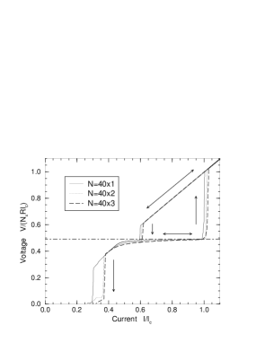
Figure 3: Calculated current-voltage characteristics for a $40\times 1$ (full line), a $40\times 2$ (dotted line) and a $40\times 3$ (long-dashed line) array, all with parameters $\tilde{g}_{x}=0.015$, $\tilde{\Omega}=0.49$, $\beta_{c}=20$, $\beta_{d}=0.05$ and $\Delta=0.05$. The horizontal dot-dashed line shows the expected position of the SIRS. Note that as the array width increases, the smallest value of $\tilde{I}$ at which all the active junctions phase-lock on the SIRS also increases, and IV characteristic on the SIRS has an increasing bend. Hence, increasing the array width at fixed $\tilde{g}_{x}$ has a effect similar to that of increasing $\tilde{g}_{x}$ at fixed width. The arrows indicate the direction of the current sweep.

The behavior shown in Fig. 3 with increasing array width is very similar to that found previously in 1D arrays with increasing coupling strength. In other words, the key parameter in understanding the curves of Fig. 3 is the product $N_{y}\tilde{g}_{x}$. For example, Fig. 3 shows that the effect of increasing $N_{y}$ while keeping $\tilde{g}_{x}$ constant is to raise slightly the maximum value of $\tilde{I}$ for which the active junctions are still locked onto the $N_{a}=40$ SIRS. Furthermore, that portion of the SIRS which corresponds to small $\tilde{I}$ is not perfectly flat (i. e. not at the expected constant voltage $V/(N_{x}RI_{c})=\tilde{\Omega}$), but instead increases slightly with increasing $\tilde{I}$ [cf. Fig. 3]. The degree of this non-flatness increases with increasing $N_{y}$. Precisely analogous effects are seen in calculations for 1D arrays with increasing $\tilde{g}_{x}$.almaas02_2 This is another piece of evidence that the key parameter is the product $N_{y}\tilde{g}_{x}$.

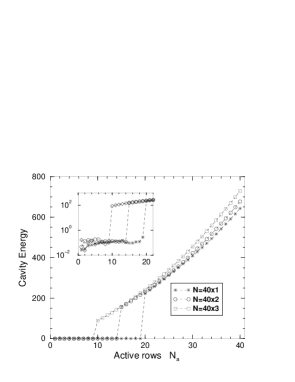
Figure 4: Time-averaged scaled energy $\tilde{E}$ in the resonant cavity as function of active number of rows for a $40\times 1$ (asterisks), a $40\times 2$ (circles) and a $40\times 3$ (squares) array with driving current $\tilde{I}=0.58$. All the other parameters are the same as those of Fig. 3. Inset: an enlargement of the IV characteristics near the synchronization threshold, on a logarithmic vertical scale. Note that the threshold number of active junctions for synchronization decreases with increasing array width.

In Fig. 4, we plot the time-averaged energy $\tilde{E}(N_{a})=\langle\tilde{a}_{R}^{2}+\tilde{a}_{I}^{2}\rangle_{\tau}$ in the cavity for three different arrays: $40\times 1$ (stars), $40\times 2$ (circles), and $40\times 3$ (squares). In all cases, $\tilde{I}=0.58$, and the other parameters are the same as those of Fig. 3. Below a threshold value of $N_{a}$, (which we denote $N_{c}$ and which depends on $N_{y}$), the active rows are in the McCumber state (not on the SIRS’s). In this case, $\tilde{E}(N_{a})$ is small and shows no obvious functional dependence on $N_{a}$ (see inset). By contrast, above threshold, $\tilde{E}(N_{a})$ is much larger and increases as $N_{a}^{2}$.

Fig. 4 shows that, when $N_{y}$ is increased at fixed $\tilde{g}_{x}$, $N_{c}$ decreases. Precisely this same trend is observed when we increase $\tilde{g}_{x}$ while holding $N_{y}$ fixed (and was observed in our previous 1D calculations with increasing $\tilde{g}_{x}$). Thus, once again, the relevant parameter in understanding the threshold behavior appears to be $N_{y}\tilde{g}_{x}$.

As in 1D arrays, it is useful to introduce a Kuramoto order parameter which describes the phase ordering. For the 2D arrays, we define a Kuramoto order parameter $\langle r_{h}\rangle_{\tau}$ for the horizontal bonds by

$$\langle r_{h}\rangle_{\tau}=\frac{1}{N_{a}N_{y}}~{}\langle|\sum_{\langle ij\rangle\parallel\hat{\bf x}}e^{i\gamma_{ij}}|\rangle_{\tau},$$ (39)

where $N_{a}$ is the number of active rows, $N_{y}$ is the number of horizontal junctions in a single row and the sum runs over all the active, horizontal junctions. [The analogous quantity $\langle r_{v}\rangle_{\tau}$ for the vertical junctions is irrelevant when $\tilde{g}_{v}=0$, since in this case these junctions are inactive.] For the parameters shown in Fig. 4, we have found, as in our previous 1D calculations, that $\langle r_{h}\rangle_{\tau}\sim 1$ for $N_{a}>N_{c}$ while $\langle r_{h}\rangle_{\tau}\ll 1$ for $N_{a}<N_{c}$. This behavior (which we do not show in a figure) reflects the fact that, for the value of $\tilde{I}$ used in Fig. 4, none of the active junctions are on a SIRS when $N_{a}<N_{c}$; hence, these junctions are not in phase with one another, and the value of $\langle r_{h}\rangle_{\tau}$ reflects this lack of coherence.

Figure 5: The time-averaged Kuramoto order parameter $\langle r_{h}\rangle_{\tau}$ (defined in Eq. (39) as a function of the number of active rows on SIRS’s for a $20\times 2$ Josephson array with $\tilde{\Omega}=0.49$, $\tilde{g}_{x}=0.01$, $\beta_{c}=20.$, $\beta_{d}=0.05$, $\Delta=0.1$ and bias current $\tilde{I}=0.53$.

For certain array parameters, $\tilde{I}$ can be chosen so that all the active junctions lie on SIRS’s, however many active rows $N_{a}$ there are. [In Fig. 2, for example, $\tilde{I}\sim 0.5$ would achieve this result.] In such cases, even though all the active junctions are oscillating with the same frequency, and locked onto SIRS’s, it is still possible to have $\langle r_{h}\rangle_{\tau}<1$. In this situation, the Kuramoto order parameter $\langle r_{h,n}\rangle_{\tau}\sim 1$ for the individual rows. This occurs because the rows are not perfectly phase-locked to one other. An example of such behavior is shown in Fig. 5, for a $20\times 2$ junction array for several numbers $N_{a}$ of active rows. The other parameters are $\tilde{\Omega}=0.49$, $\tilde{g}_{x}=0.01$, $\beta_{c}=20.$, $\beta_{d}=0.05$, $\Delta=0.1$ and $\tilde{I}=0.53$. As the number of active rows on the SIRS’s increases, $\langle r_{x}\rangle_{\tau}\rightarrow 1$. [Also, of course, $\langle r_{x}\rangle_{\tau}=1$ for one active row on a SIRS.] Numerically, we find that it is easier in 2D than in 1D to achieve a state with all active junctions biased on a SIRS, but with $\langle r_{x}\rangle_{\tau}<1$. In all such cases, we can easily cause $\langle r_{x}\rangle_{\tau}\rightarrow 1$ simply by increasing $\tilde{g}_{x}$.

Figure 6: Phase plot of points $(\gamma,\dot{\gamma})$ where $\gamma$ is the gauge-invariant phase difference across a junction, shown for (a) a vertical junction and (b) a horizontal junction, in an array in which the cavity couples only to the horizontal junctions: $\tilde{g}_{x}=0.$, $\tilde{g}_{y}=0.5$. The array size is $10\times 4$, and the other parameters are $\tilde{\Omega}=0.45$, $\Delta=0.05$, $\beta_{c}=20$, $\beta_{d}=0.05$ and $\tilde{I}=0.46$. The vertical junction in (a) displays aperiodic motion with very small amplitude, corresponding to no time-averaged voltage drop across that junction, while the horizontal junction in (b) has a phase difference which varies periodically in time.

The threshold shown in Fig. 4 corresponds to a transition from a state in which none of the active junctions are on SIRS’s to a state in which all are on SIRS’s. It is possible to choose $\tilde{I}$ so as to have any number of active rows $N_{a}$ on SIRS’s. In this case, the cavity energy $\tilde{E}(N_{a})$, in our model, is approximately quadratic in $N_{a}$, with no obvious threshold behavior. This feature of our results is discussed further below.

IV.2 Vertical coupling

We have also investigated the case of $\tilde{g}_{x}=0$, $\tilde{g}_{y}\neq 0$, for a wide range range of $\tilde{g}_{y}$ values. For our geometry, we have not been able to find any value for $\tilde{g}_{y}$ for which a SIRS develops. In essence, when the cavity couples only to the vertical junctions, it is invisible in the IV characteristics. This behavior is easily understood. In this geometry, with current applied in the $x$ direction, both the time-averaged voltage and the time-averaged current through the vertical junctions are very small. Hence, too little power is dissipated in the vertical junctions to induce a resonance with the cavity.

To illustrate this behavior, we show in Fig. 6 some representative phase plots of $(\gamma_{ij},\dot{\gamma}_{ij})$ for (a) a vertical junction and (b) a horizontal junction in a $10\times 4$ array with $\tilde{g}_{x}=0$, $\tilde{g}_{y}=0.5$, $\beta_{c}=20$, $\beta_{d}=0.05$, $\tilde{\Omega}=0.45$, $\Delta=0.05$ at bias current $\tilde{I}=0.46$ (close to a possible resonance with cavity). The phase plot for the vertical junction exhibits small-amplitude aperiodic motion, while that of the horizontal junction shows that this junction is in its active state and undergoing periodic motion in phase space. This lack of response by the $y$ junctions to the cavity probably explains why the 1D simulations describe the experiments so well.

It is no surprise that the cavity interacts only very weakly with the vertical junctions. From previous studies of both underdamped and overdamped disordered Josephson arrays in a rectangular geometry (see, e. g., Refs. wenbin94, , and wenbin92, ), it is known that when current is applied in the $x$ direction, the $y$ junctions remain superconducting, with $\langle V\rangle_{\tau}\approx 0$, while the $x$ junctions comprising an active row are almost perfectly synchronized, with $\langle r_{x}\rangle\approx 1$.

If there were an an external magnetic field perpendicular to the array, we believe that SIRS’s would be generated for $\tilde{g}_{y}\neq 0$, even if $\tilde{g}_{x}=0$. In this case, the magnetic field would induce frustration. Specifically, since the sum of the gauge invariant phase differences around a plaquette must be an integer multiple of $2\pi$, the presence of magnetic-field-induced vortices piercing the plaquettes would induce nonzero voltages across, and supercurrents in, the $y$ junctions. It would be of great interest if calculations were carried out in such applied magnetic fields.

IV.3 Comparison with 1D Model

We now compare our 2D results explicitly with those for 1D arrays. In our earlier 1D model, we found numericallyalmaas02_2 that the threshold number of active junctions $N_{c}$ was inversely proportional to the coupling constant $\tilde{g}$. This behavior is reasonable because the inhomogeneous term driving the cavity variable $\tilde{a}_{R}$ is proportional to the product of $\tilde{g}$ and $N_{a}$.

Some of our numerical trends in the 2D case can be understood similarly. For example, the inhomogeneous term in Eq. (37) is the last term on the right-hand side. It is proportional to the sum of the coupling constants $\tilde{g}_{ij}$ over all the junctions parallel to $\tilde{I}$. Thus, for $\tilde{g}_{x}\neq 0$, $\tilde{g}_{y}=0$, and for the same driving current $\tilde{I}$, we expect that an $N_{x}\times N_{y}$ array with a coupling constant $\tilde{g}_{x}$ should behave like an $N_{x}\times 1$ array with coupling constant $N_{y}\tilde{g}_{x}$.

Figure 7: IV characteristics for a $10\times 1$ array ($\ast$) and a $10\times 10$ array ($\circ$). The $10\times 1)$ array has parameters $\tilde{g}_{x,10\times 1}=0.0259$, $\tilde{\Omega}=0.41$, $\beta_{c}=20$, $\beta_{d}=0.05$ and $\Delta=0.05$. The expected position of the SIRS’s are marked by horizontal dashed lines. The $10\times 10$ array has $\tilde{g}_{x,10\times 10}$ = 0.00259, and the other parameters are the same as for the $10\times 1$ array. The IV characteristics are shown for both increasing and decreasing current drive, as discussed in the text.

To check this hypothesis, we compare, in Fig. 7, the IV characteristics of a $10\times 1$ array having coupling constant $\tilde{g}_{x;10\times 1}=0.0259$ with those of a $10\times 10$ array with coupling constant $\tilde{g}_{x;10\times 10}=0.00259$. The other parameters are the same for the two arrays: $\tilde{\Omega}=0.41$, $\beta_{c}=20$, $\beta_{d}=0.05$ and $\Delta=0.05$. The expected positions of the SIRS’s [at $V/(NRI_{c})=\tilde{\Omega}$] are indicated by dashed horizontal lines. Indeed, the two sets of IV characteristics are very similar. Even some of the subtle differences can be understood in a simple way. For example, the $10\times 10$ IV’s are slightly flatter than the $10\times 1$ curves. We believe this extra flatness occurs because the individual junction couplings in the $10\times 1$ array are $10$ times larger than those in the $10\times 10$ array. From our previous 1D simulations, the IV’s on the steps become more and more rounded as $\tilde{g}_{x}$ increases, i. e., the voltage on the lower portion of the SIRS is no longer independent of $\tilde{I}$ [cf. Ref. almaas02_2, ]. Precisely this behavior is seen in Fig. 7.

Another subtle difference between the 1D and 2D curves of Fig. 7 is the values of the so-called “retrapping current” in the two sets of curves (i. e. the current values below which the McCumber curve becomes unstable). We believe that this difference can be understood in terms of the effects of disorder in the junction critical currents in 1D and 2D. Specifically, for a given value of $\Delta$, the 2D arrays are effectively less disordered than the 1D arrays, since the average critical current for a single row has a smaller rms spread than the critical current of a single junction in a 1D array.

An important similarity between the two sets of curves is that, in both the $10\times 10$ and the $10\times 1$ arrays, the width of the SIRS’s varies similarly (and non-monotonically) with the number of active rows. This behavior distinguishes our predictions from some other models,filatrella ; filatrella2 in which the cavity is modeled as an RLC oscillator connected in parallel to the entire array, and which predicts a monotonic dependence of SIRS width on $N_{a}$. barbara02

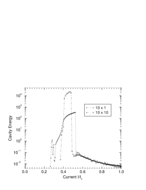
Figure 8: Time-averaged reduced cavity energy $\tilde{E}$, for a $10\times 1$ array and a $10\times 10$ array for the same choice of array parameters as in Fig. 7. The calculations are carried out on the decreasing current branch with all rows active. Note that $\tilde{g}_{x}$ for the $10\times 10$ array is 10 times smaller than that of the $10\times 1$ array.

In Fig. 8 we plot the reduced time-averaged cavity energy $\tilde{E}=\langle a_{R}^{2}+a_{I}^{2}\rangle_{\tau}$ as a function of $\tilde{I}=I/I_{c}$ for both arrays of Fig. 7, under conditions such that all rows are active. This plot is obtained by following the decreasing current branch. Surprisingly, when the $10\times 10$ array (with $\tilde{g}_{(10\times 10)}=0.1~{}\tilde{g}_{(10\times 1)}$) locks on to the SIRS, $\tilde{E}$ jumps to a value which is approximately two orders of magnitude larger than that of the corresponding jump in the $10\times 1$ array, even though the parameter $N_{y}\tilde{g}_{x}$ is the same for both arrays. We believe that the difference is due simply to the greater number of junctions which are driving the cavity in the 2D case. Even though the width of the steps is controlled primarily by the parameter $N_{y}\tilde{g}_{x}$, the energy in the cavity is determined by the square of the number of radiating junctions. This square is 100 times larger for the 2D array than for the 1D array.

V Summary

In this paper, we have derived equations of motions for a 2D array of underdamped Josephson junctions in a single-mode resonant cavity, starting from a suitable model Hamiltonian and including the effects of both a current drive and resistive dissipation. In the limit of zero junction-cavity coupling, these equations of motion correctly reduce to those describing a 2D array of resistively and capacitively shunted Josephson junctions.

As in our previous 1D model, the present equations of motion lead to a transition from incoherence to coherence, as a function of the number of active rows $N_{a}$. This transition again results from the effectively mean-field-like nature of the interaction between the junctions and the cavity. Specifically, because each junction is, in effect, coupled to every other active junction via the cavity, the strength of the effective coupling is proportional to the number of active junctions. Thus, for any $\tilde{g}_{x}$, no matter how small, a transition to coherence is to be expected for sufficiently large number of active rows $N_{a}$. We also found a striking effect of polarization: the transition to coherence occurs only when the cavity mode is polarized so that its electric field has a component parallel to the direction of current flow.

Next, we briefly compare our numerical results to the behavior seen in experiments.barbara ; vasilic02 Our calculations show the following features seen in experiments: (i) self-induced resonant steps (SIRS’s) in the IV characteristics; (ii) a transition from incoherence to coherence above a threshold number of active junctions; and (iii) a total energy in the cavity which varies quadratically with the number of active junctions when those junctions are locked onto SIRS’s. There may, however, be some differences as well. In particular, our transition to a quadratic behavior occurs when the active junctions are locked onto SIRS’s. In possible contrast to our results, in some experimental arrays,vasilic02 it has been reported that even below the “coherence threshold,” individual rows of junctions are locked onto SIRS’s, but these SIRS’s are not coherent with one another, and hence, do not radiate an amount of power into the cavity proportional to the square of the number of junctions on the SIRS’s. Thus far, in our calculations, we have found that when $N_{a}$ junctions are locked onto the steps, the energy in the cavity is quadratic in $N_{a}$. The threshold, in our calculations, occurs when all the active junctions lock onto SIRS’s, not when active junctions which are already locked onto SIRS’s become coherent with one another.

For some choices of the parameters $\tilde{g}_{x}$, $\tilde{\Omega}$, $\Delta$, $\beta$, and $\tilde{I}$, we find dynamical states such that all active rows lock onto SIRS’s while $\langle r\rangle_{\tau}<1$. In such states, the Kuramoto order parameter for the individual rows is still $\langle r\rangle_{\tau}\sim 1$, implying that the rows are not perfectly phase-locked to each other. An example of such a state is shown in Fig. 5. In such states, our calculated energy $\tilde{E}$ in the cavity appears to vary smoothly with $N_{a}$, and exhibits no threshold behavior, in contrast to what we find at other applied currents [cf. Fig. 4]. This behavior appears to differ from what was reported experimentally in a recent paper;vasilic02 the reasons for the difference are not clear to us.

In summary, we have extended our previous theory of Josephson junction arrays coupled to a resonant cavity to the case of 2D arrays. The 2D theory bears many similarities to the 1D case, and makes clear why the 1D model works so well. These similarities arise because, in a square array, the coupling to the cavity takes place only through those junctions which are parallel to the applied current. Again as in 1D, our model leads to clearly defined SIRS’s whose voltages are proportional to the resonant frequency of the cavity. Another similarity is that, in 2D as in 1D, when a fixed number of rows are biased on a SIRS, the cavity energy is linear in the input power.

We also find some results which are specific to 2D. For example, whenever one junction in a given row is biased on a SIRS, all the junctions in that row phase-lock onto that same SIRS. In addition, the time-averaged energy contained in the resonant cavity is quadratic in the number of active rows, but, when the array is biased on a SIRS, is much larger in the 2D array than in the 1D array, for the same value of the coupling parameter $\tilde{g}_{x}N_{y}$.

When the cavity mode is polarized perpendicular to the direction of current drive, we find that the cavity does not affect the array IV characteristics. Our equations suggest that this non-effect might change if the array were frustrated, e. g., by an external magnetic field normal to the array. Such frustration would cause junctions in the $x$ and $y$ direction to be coupled. It would be of great interest if this speculation could be tested experimentally.

- (1) For an extensive review, see, e. g. R. S. Newrock, C. J. Lobb, U. Geigenmüller, and M. Octavio, Solid State Physics 54, 263 (2000).
- (2) See, for example, P. M. Chaikin and T. C. Lubensky. Principles of Condensed Matter Physics. Cambridge Univ. Press, New York, 1995.
- (3) M. Tinkham. Introduction to Superconductivity. McGraw-Hill, New York, Second edition, 1996.
- (4) P. Barbara, A. B. Cawthorne, S. V. Shitov, and C. J. Lobb. Phys. Rev. Lett. 82, 1963 (1999).
- (5) P. Barbara, G. Filatrella, C. J. Lobb, and N. F. Pedersen, “Cavity Synchronization of Underdamped Josephson-Junction Arrays,” to be published in Studies in High-Temperature Superconductors, edited by V. Narlikar (NOVA Science Publishers, New York, in press).
- (6) B. Vasilic, P. Barbara, S. V. Shitov, and C. J. Lobb. Published in the proceedings of Applied Superconductivity Conference 2000.
- (7) B. Vasilić, P. Barbara, S. V. Shitov, and C. J. Lobb. Phys. Rev. B 65, 180503(R) (2002).
- (8) B. Vasilic, P. Barbara, S. V. Shitov, E. Ott, T. M. Antonsen, and C. J. Lobb. Abstract Y27.001 of the APS March Meeting, Seattle, WA., March 2001.
- (9) G. Filatrella, N. F. Pedersen, and K. Wiesenfeld. Phys. Rev. E 61, 2513 (2000).
- (10) G. Filatrella, N. F. Pedersen, and K. Wiesenfeld. IEEE Trans. Appl. Supercond.
- (11) E. Almaas and D. Stroud. Phys. Rev. B 63, 144522 (2001). See also E. Almaas and D. Stroud, Phys. Rev. B 64, 179902(E) (2001).
- (12) E. Almaas and D. Stroud. Phys. Rev. B 65, 134502 (2002).
- (13) J. C. Slater. Microwave Electronics. D. Van Nostrand, New York, 1950.
- (14) A. Yariv. Quantum Electronics. J. Wiley & Sons, New York, Second edition, 1975.
- (15) V. Ambegaokar, U. Eckern, and G. Schön. Phys. Rev. Lett. 48, 1745 (1982).
- (16) A. O. Caldeira and A. J. Leggett. Phys. Rev. Lett. 46, 211 (1981).
- (17) A. O. Caldeira and A. J. Leggett. Ann. Phys. (N. Y.) 149, 374 (1983).
- (18) S. Chakravarty, G.-L. Ingold, S. Kivelson, and A. Luther. Phys. Rev. Lett. 56, 2303 (1986).
- (19) R. Fazio and G. Schön. Phys. Rev. B 43, 5307 (1990).
- (20) B. J. Kim and M. Y. Choi. Phys. Rev. B 52, 3624 (1995).
- (21) W. H. Press, S. A. Teukolsky, W. T. Vetterling, and B. P. Flannery. Numerical Recipes. Cambridge Univ. Press, New York, 1992.
- (22) Note that one always has the relation .
- (23) See, for example, S. Teitel and C. Jayaprakash, Phys. Rev. B27, 598 (1983).
- (24) T. S. Tighe, A. T. Johnson, and M. Tinkham. Phys. Rev. B 44, 10286 (1991).
- (25) W. Yu and D. Stroud. Phys. Rev. B 46, 14005 (1992).
- (26) V. Ambegaokar and A. Baratoff, Phys. Rev. Lett. 10, 486 (1963).
- (27) J. R. Waldram. Superconductivity of Metals and Cuprates. Inst. of Phys. Publ., Philadelphia, 1996.
- (28) W. Yu. Topics in the Dynamical Properties of Josephson Networks. PhD thesis, The Ohio State University, 1994.