Perturbation Theory on the Superconductivity of Heavy Fermion Superconductors ${\rm CeIr}_{x}{\rm Co}_{1-x}{\rm In}_{5}$

Abstract

We reformulate the Éliashberg’s equation for the superconducting transition within the quasi-particle description, which takes account of the heavy electron mass. We discuss the superconductivity of ${\rm CeIr}_{x}{\rm Co}_{1-x}{\rm In}_{5}$ by using such a renormalized formula. On the basis of an effective two-dimensional Hubbard model which represents the most heavy quasi-two dimensional Fermi surface with $f$-character of ${\rm CeIr}_{x}{\rm Co}_{1-x}{\rm In}_{5}$, both normal and anomalous self-energies are calculated up to third order with respect to the renormalized on-site repulsion $U$ between quasi-particles. The superconducting transition temperature is obtained by solving the ${\rm\acute{E}}$liashberg’s equation. Reasonable transition temperatures are obtained for moderately large $U$. It is found that the momentum and frequency dependence of spin fluctuations given by RPA-like terms gives rise to the d-wave pairing state, while the vertex correction terms are important for obtaining reasonable transition temperatures and for differentiating $n$-dependence of $T_{{\rm c}}$. These obtained results seem to explain the $x$-dependence of $T_{{\rm c}}$ in ${\rm CeIr}_{x}{\rm Co}_{1-x}{\rm In}_{5}$ and confirm the usefulness of the perturbation theory with respect to $U$.

1 Introduction

In heavy fermion system, the effective mass is enhanced by $10^{2}\sim 10^{3}$ times as large as that of free electron. The coefficient of $T^{2}$-law of resistivity is also enhanced by $10^{4}\sim 10^{6}$ times as large as that of conventional metal. Such a large electron mass and coefficient of $T^{2}$-law of resistivity stem from the electron correlation. In heavy fermion superconductors, itinerant electrons compose such a Fermi liquid and then undergo the superconducting transition. From this point of view, we can expect that superconductivities in heavy fermion systems are derived also from the electron correlation through the momentum and frequency dependence of the effective interaction between electrons. Therefore, in contrast to the cuprates, it is not clear whether taking only the effect of the specific diagrams which are favorable to the spin fluctuations is reliable for revealing the mechanism of superconductivity in the heavy fermion superconductors.

In this paper, we present an essentially important point in theoretical study of superconductivity in heavy fermion systems. In contrast to the cuprates, the momentum dependence of the mass enhancement factor in heavy fermion systems is weak because of the localized nature of $f$-electrons. In this case we can reformulate the ${\rm\acute{E}}$liashberg’s equation also in the renormalized form, where we have already included the large mass enhancement effect. By using the renormalized Fermi energy as unit of energy the critical temperature $T_{{\rm c}}$ determined by the perturbation is the same as that obtained after taking account of the mass enhancement effect. Thus, we can formulate the perturbation theory which is consistent with the large mass enhancement. The formulation is one of purposes of the present paper. Therefore, we calculate the superconducting transition temperature $T_{{\rm c}}$ of heavy fermion superconductors by the perturbation theory based on Fermi liquid theory. In our formalism, the effective interaction corresponding to the superexchange interaction  [1] is included in the vertex terms in principle, because we start from renormalized Fermi liquid and treat only the Coulomb repulsion by the perturbation theory.

The perturbation approach is sensitive to the dispersion of the bare energy band by its nature, it implies that the lattice structures and the band filling play the essential roles in the calculation of $T_{{\rm c}}$. Therefore it is important to evaluate $T_{{\rm c}}$ on the basis of the detailed electronic structure in each system. In this paper, we calculate $T_{{\rm c}}$ of ${\rm CeIr}_{x}{\rm Co}_{1-x}{\rm In}_{5}$.

The organization of this paper is as follows. In $\S 2$, a theoretical treatment of heavy fermion superconductivity is presented. In $\S 3$, $T_{{\rm c}}$ of ${\rm CeIr}_{x}{\rm Co}_{1-x}{\rm In}_{5}$ is calculated, after giving the model Hamiltonian, perturbation expansion terms and ${\rm\acute{E}}$liashberg’s equation. Moreover the selfenergy, density of states and other quantities are shown. Finally in $\S 4$, summary, discussions and conclusion are presented.

2 A theory of heavy fermion superconductivity

In this section, we discuss a theoretical treatment of heavy fermion superconductivity. As indicated in various experiments, such as a jump of the specific heat at the transition temperature ($T_{\rm c}$), the superconductivity can be interpreted as a transition of quasi-particles with heavy electron mass. We here formulate the way to calculate the superconducting transition temperature $T_{\rm c}$ on the heavy fermion quasi-particle state in the periodic Anderson model (PAM).

One of the characteristics in heavy fermion systems is the weak momentum dependence, corresponding to degree of the local $f$-electron spins at high temperatures or energies. The perturbation expansion in the hybridization matrix element in PAM leads to the RKKY interaction between these local spins. This expansion is valid at high temperatures, and may be the origin of the magnetic transition in $f$-electron systems. However, if no magnetic transition occurs, the system goes to a singlet ground state as the whole. This just is the Fermi liquid state with heavy electron mass. In this case, we had better treat it by the perturbation theory with respect to the on-site Coulomb repulsion $U$ between $f$-electrons, because of the analyticity about $U$. The analytic property has been exactly proved in impurity Anderson model [2, 3, 4, 5]. Although there is no exact such proof in PAM, the principle of the adiabatic continuation confirms the correctness of the perturbation theory in $U$.

From such a point of view, one of the authors (K.Y.) has described the Fermi liquid theory for the heavy fermion state in PAM [6]. The momentum independent part of the 4-point vertex functions $\Gamma_{\sigma\sigma^{\prime}}^{\rm loc}$ between $f$-electrons with the spin $\sigma$ and $\sigma^{\prime}$ plays an important role. This s-wave scattering part, corresponding to the above-mentioned local character at high energies, leads to the featureless large mass enhancement factor $\tilde{\gamma}=a^{-1}$. In fact, when the momentum dependence of the mass enhancement factor can be ignored, the $T$-linear coefficient of the specific heat in PAM, is given by $\gamma\simeq(2/3)\pi^{2}k_{\rm B}^{2}{\rho^{f}(0)}^{2}\Gamma_{\uparrow\downarrow}^{\rm loc}=(2/3)\pi^{2}k_{\rm B}^{2}\rho^{f}(0)\tilde{\gamma}$, where $k_{\rm B}$ is the Boltzmann’s constant, and $\rho^{f}(0)$ the $f$-electron density of states at the Fermi level. This indicates that the large mass enhancement factor $\tilde{\gamma}=a^{-1}$ is represented as $\rho^{f}(0)\Gamma_{\uparrow\downarrow}^{\rm loc}$ with use of the s-wave scattering part of the 4-point vertex. Thus, we can see that the vertex $\Gamma_{\uparrow\downarrow}^{\rm loc}$ is enhanced by $\tilde{\gamma}=a^{-1}$. This corresponds to the fact that the interaction $a^{2}\Gamma_{\uparrow\downarrow}^{\rm loc}$ between the quasi-particles has the order of magnitude of the effective band-width of quasi-particles $T_{0}\simeq 1/\tilde{\gamma}\rho^{f}(0)$; $T_{0}$ is the characteristic energy scale of the heavy fermion state, and below $T_{0}$, the low energy excitation can be described by the Fermi liquid theory. On the other hand, the imaginary part of the $f$-electron self-energy, which is proportional to the $T^{2}$-term of the electrical resistivity, is given by $\Delta_{k}=(4\pi^{2}/3)\rho^{f}(0)^{2}\pi{\Gamma_{\uparrow\downarrow}^{\rm loc}}^{2}T^{2}$, if the momentum dependence of the vertices can be ignored. Thus, the coefficient $A$ of the $T^{2}$-term of the electrical resistivity is proportional to $\gamma^{2}$ through the vertex $\Gamma_{\uparrow\downarrow}^{\rm loc}$. This relation $A\propto\gamma^{2}$ is just the Kadowaki-Wood’s relation, which holds in the case where the momentum dependence of the vertices is sufficiently weak to be ignored. Actually, in the heavy fermion systems, the Kadowaki-Wood’s relation is confirmed. This fact means that the 4-point vertex function, i.e., the interaction between quasi-particles possesses the above-mentioned local nature.

The superconductivity in the heavy fermion systems appears under this situation below $T_{0}$. The s-wave large repulsive part $\Gamma_{\uparrow\downarrow}^{\rm loc}$ prevents the appearance of the s-wave singlet superconductivity in strongly correlated systems. In this case, an anisotropic (such as p-, d-wave and so on) superconductivity will be realized due to the remaining momentum dependence of the 4-point vertices. We here discuss such a transition to the anisotropic superconductivity on the basis of the heavy fermion quasi-particle state renormalized by the large s-wave scattering part $\Gamma_{\uparrow\downarrow}^{\rm loc}$.

First of all, we divide the 4-point full vertex function $\Gamma_{\sigma\sigma^{\prime}}(p_{1},p_{2};p_{3},p_{4})$ into the large s-wave scattering part $\Gamma_{\sigma\sigma^{\prime}}^{\rm loc}$ and the non-s wave part $\Delta\Gamma_{\sigma\sigma^{\prime}}(p_{1},p_{2};p_{3},p_{4})$;

$$\Gamma_{\sigma\sigma^{\prime}}(p_{1},p_{2};p_{3},p_{4})=\Gamma_{\sigma\sigma^{\prime}}^{\rm loc}+\Delta\Gamma_{\sigma\sigma^{\prime}}(p_{1},p_{2};p_{3},p_{4}),$$ (1)

where $p_{1}$ and $p_{2}$ are the incident momenta, and $p_{3}$, $p_{4}$ the outgoing. The momentum dependent part has rather remarkable momentum dependence as the heavy fermion quasi-particles grow below $T_{0}$. The effective Cooper pairing interaction in the anisotropic superconductivity results from the momentum dependence of $\Delta\Gamma_{\sigma\sigma^{\prime}}(p_{1},p_{2};p_{3},p_{4})$. Our purpose is to formulate how to calculate $\Delta\Gamma_{\sigma\sigma^{\prime}}(p_{1},p_{2};p_{3},p_{4})$ for the heavy fermion quasi-particles, which are renormalized by the large local part $\Gamma_{\uparrow\downarrow}^{\rm loc}$. Corresponding to these two terms of the full vertex function, we can also separate the self-energy into the local part and the non-local part

$$\Sigma(k,\omega)=\Sigma_{\rm loc}(\omega)+\Delta\Sigma(k,\omega).$$ (2)

In this case, the $f$-electron Green’s function below $T_{0}$ is given by

$$G(k,\omega) = \frac{1}{\omega-\xi_{k}-\Sigma^{\rm loc}(\omega)-\Delta\Sigma(k,\omega)-\frac{V_{k}^{2}}{\omega-\epsilon_{k}}},$$ (3)

$$= \frac{a}{\omega-\tilde{E}_{k}-\tilde{\Sigma}(k,\omega)-\frac{\tilde{V}_{k}^{2}}{\omega-\epsilon_{k}}}+G_{\rm inc}(\omega),$$

where $a$ is a wave function renormalization factor, and $\tilde{E}_{k}=a(\xi_{k}+{\rm Re}\Sigma^{\rm loc}(0))$, $\tilde{V}_{k}=\sqrt{a}V_{k}$ and $\tilde{\Sigma}(k,\omega)=a\Delta\Sigma(k,\omega)$ are, respectively, a renormalized $f$-electron band, hybridization term and self-energy. $G_{\rm inc}(\omega)$ is a featureless incoherent part. The imaginary part of $\Sigma^{\rm loc}$ proportional to $\omega^{2}$ can be included in the remaining renormalized self-energy $\tilde{\Sigma}(k,\omega)$, as indicated by Hewson for the impurity Anderson model [7, 8]. From the Ward-Takahashi identity, we can obtain the large mass enhancement factor,

$$\tilde{\gamma}=a^{-1}=1-\dfrac{d\Sigma_{\rm loc}(0)}{d\omega}=1-\dfrac{i}{2}\int d\omega\Gamma_{\uparrow\downarrow}^{\rm loc}G_{\rm inc}^{2}(\omega).$$ (4)

The above equation of the Green’s function is the counterpart on the quasi-particle description. In addition, we can set the large local vertex $\Gamma_{\uparrow\downarrow}^{\rm loc}$ as a constant value at zero frequencies, as far as the frequency of external lines is less than $T_{0}$. In this case, the effective on-site interaction $a^{2}\Gamma_{\uparrow\downarrow}^{\rm loc}$ works between the quasi-particles. In the impurity Anderson model, $a^{2}\Gamma_{\uparrow\downarrow}^{\rm loc}=a\pi\Delta=4T_{\rm K}$, where $\Delta$ and $T_{\rm K}$ are, respectively, the width of the virtual bound state and the Kondo temperature. Therefore, we can assume that $a^{2}\Gamma_{\uparrow\downarrow}^{\rm loc}$ has the order of $T_{0}$. This is also consistent with the above-mentioned discussion of the coefficient of the specific heat.

We now show that in the region $\omega\leq T_{0}$, the renormalized self-energy $\tilde{\Sigma}(k,\omega)$ and vertex function $\tilde{\Gamma}_{\sigma\sigma^{\prime}}(p_{1},p_{2};p_{3},p_{4})=a^{2}\Delta\Gamma_{\sigma\sigma^{\prime}}(p_{1},p_{2};p_{3},p_{4})$ can be discussed with the perturbation expansion with respect to the effective on-site interaction $\tilde{\Gamma}_{\uparrow\downarrow}^{\rm loc}=a^{2}\Gamma_{\uparrow\downarrow}^{\rm loc}$. This expansion can be also considered as the one with respect to the momentum dependence which is governed by the renormalized Fermi surface. First, let us consider the renormalized self-energy $\tilde{\Sigma}(k,\omega)=a\Delta\Sigma(k,\omega)$. Because we have divided the Green’s function into the two parts $a\tilde{G}(k,\omega)+G_{\rm inc}(\omega)$, we can correspondingly divide any diagrams in the expansion with respect to the bare interaction $U$ into diagrams with and without the momentum dependence. The latter is contained in the local self-energy $\Sigma_{\rm loc}(\omega)$, on the other hand, the former can be rewritten as the expansion with respect to the effective interaction $\tilde{\Gamma}_{\uparrow\downarrow}^{\rm loc}$ by concentrating diagrams with the same momentum dependence. As shown in Fig. 1, for instance, the $U^{2}$-type diagram has the same momentum dependence as the ${\Gamma_{\uparrow\downarrow}^{\rm loc}}^{2}$-type, each vertex of which includes all the s-wave scattering process. Because three lines of the renormalized Green’s function $a\tilde{G}(k,\omega)$ yields $a^{3}$, and the renormalized self-energy $\tilde{\Sigma}(k,\omega)$ includes $a$, the ${\Gamma_{\uparrow\downarrow}^{\rm loc}}^{2}$-type is estimated by calculating $a^{4}{\Gamma_{\uparrow\downarrow}^{\rm loc}}^{2}\tilde{G}\tilde{G}\tilde{G}$. This just corresponds to the diagram of the order two with respect to the effective interaction $\tilde{\Gamma}_{\uparrow\downarrow}^{\rm loc}=a^{2}\Gamma_{\uparrow\downarrow}^{\rm loc}$. In the same way, the full vertex $\tilde{\Gamma}_{\sigma\sigma^{\prime}}(p_{1},p_{2};p_{3},p_{4})$ can be also re-written as the expansion with respect to the quasi-particle Green’s function $\tilde{G}(k,\omega)$ and the quasi-particle s-wave scattering interaction $\tilde{\Gamma}_{\sigma\sigma^{\prime}}^{\rm loc}$ as shown in Fig. 2. Thus, we can discuss the phenomena below $T_{0}$ within the renormalized effective PAM, so far as the frequency of external lines is less than $T_{0}$. The validity of such a perturbation expansion with respect to the renormalized interaction is shown by the fact that the fixed point Hamiltonian in the renormalization group can be written as the renormalized PAM. In this case, the locality of the relevant interaction is very important. In the heavy fermion systems, this condition almost holds as shown in the Kadowaki-Wood’s relation. We formulate below the superconducting transition on the quasi-particle description discussed above.

The superconducting transition is always marked by divergence of the full vertex $\Gamma_{\sigma\sigma^{\prime}}(p,-p;p^{\prime},-p^{\prime})\equiv\Gamma_{\sigma\sigma^{\prime}}(p,p^{\prime})$. We can rewrite it as divergence of the quasi-particle full vertex $\tilde{\Gamma}_{\sigma\sigma^{\prime}}(p,p^{\prime})$. As usual, we estimate the Éliashberg equation,

$$\sum_{p^{\prime}}\Gamma^{(2)}(p,p^{\prime})|G(p^{\prime},i\omega^{\prime}_{n})|^{2}\Delta(p^{\prime},i\omega^{\prime}_{n})=\Delta(p,i\omega_{n}),$$ (5)

where $\Delta(p,i\omega_{n})$ is an anomalous self-energy with a fermion Matsubara frequency $\omega_{n}=(2n+1)\pi T$, and the Cooper pairing effective interaction $\Gamma^{(2)}(p,p^{\prime})$ is the particle-particle irreducible vertex. The Eq.( 5 ) includes the integral of $|G(p^{\prime},i\omega^{\prime}_{n})|^{2}$. The most important part of this integral comes from the part mediated by quasi-particles $a^{2}|\tilde{G}(p^{\prime},i\omega^{\prime}_{n})|^{2}$. The Éliashberg equation can be re-written as

$$\sum_{p^{\prime}}a^{2}\Gamma^{(2)}(p,p^{\prime})|\tilde{G}(p^{\prime},i\omega^{\prime}_{n})|^{2}\Delta(p^{\prime},i\omega^{\prime}_{n})=\Delta(p,i\omega_{n}).$$ (6)

This $a^{2}\Gamma^{(2)}(p,p^{\prime})$ is the particle-particle irreducible vertex between quasi-particles with the external frequencies less than $T_{0}$. As discussed above, for such a vertex, we can also apply the perturbation expansion with respect to the renormalized on-site repulsion $a^{2}\Gamma_{\uparrow\downarrow}^{\rm loc}$ between quasi-particles.

In order to treat the heavy fermion superconductivity, we have approximately introduced the quasi-particle state renormalized by the s-wave scattering part, which itself does not yield the pairing interaction. Starting from the quasi-particle state, we calculate the momentum dependent interaction between quasi-particles by the perturbation theory and derive the anisotropic superconductivity. It should be noted that even if the effective interaction depends on momentum as seen in the cuprates, we can treat such a separation of the vertices in the momentum space, as far as, at the final stage, everything is included in a consistent way.

3 Calculating $T_{{\rm c}}$ of ${\rm CeIr}_{x}{\rm Co}_{1-x}{\rm In}_{5}$

3.1 Introduction to ${\rm Ce(Rh,Ir,Co)In_{5}}$

Superconductivities are discovered in a series of ${\rm CeMIn_{5}}$ tetragonal compounds for M=${\rm Co,Rh}$ or ${\rm Ir}$. ${\rm CeIrIn_{5}}$ [9] and ${\rm CeCoIn_{5}}$ [10] are superconductors at ambient pressure. The transition temperature $T_{{\rm c}}$ (and the electronic specific heat coefficients $\gamma$) are 0.4K (680${\rm mJ/K^{2}mol}$), and 2.3K (300-1000${\rm mJ/K^{2}mol}$), respectively. In contrast, ${\rm CeRhIn_{5}}$ [11] orders antiferromagnetically below $T_{{\rm N}}=3.8$K, whereas the superconductivity is observed under pressure, $p\geq 1.6$GPa. The observations of power law temperature dependence of the specific heat, thermal conductivity, and NMR relaxation rate have identified ${\rm Ce(Rh,Ir,Co)In_{5}}$ as unconventional superconductors with line nodes. The thermal conductivity measurement in a magnetic field rotating within the 2D planes also reveals that the superconducting gap symmetry of ${\rm CeCoIn_{5}}$ most likely belongs to $d_{x^{2}-y^{2}}$ [12]. The temperature-composition phase diagram for ${\rm Ce(Rh,Ir,Co)In_{5}}$ has been obtained mainly from heat capacity measurements on single crystals [13]. The phase diagram shows an interesting asymmetry with respect to the coupling between magnetism and superconductivity: in the case of ${\rm Rh}$-${\rm Ir}$, $T_{{\rm c}}$ increases as the magnetic boundary is approached, whereas in ${\rm Rh}$-${\rm Co}$ case, ${\rm T_{{\rm c}}}$ decreases. According to the phase diagram, the superconducting phase of ${\rm CeIr}_{x}{\rm Co}_{1-x}{\rm In}_{5}$ is apart from the antiferromagnetic ordered phase. When $x$ increases from $0$ to $1$, $T_{{\rm c}}$ decreases from 2.3 K to 0.4 K. The temperature dependence of the resistivity $\rho$ of ${\rm CeIrIn_{5}}$ follows the dependence $\rho=\rho_{0}+AT^{2}$. There exists a large anisotropy in the resistivity of ${\rm CeIrIn_{5}}$. This anisotropy is closely related to the quasi-two dimensional Fermi surface. The band calculations were performed for ${\rm CeIrIn_{5}}$ [14] and ${\rm CeCoIn_{5}}$  [15]. The Fermi surfaces calculated for ${\rm CeIrIn_{5}}$ and ${\rm CeCoIn_{5}}$, respectively are almost same. The topology of the Fermi surface is explained by the 4$f$-itinerant band model. The calculated Fermi surfaces consist of nearly cylindrical Fermi surfaces and small ellipsoidal ones.

3.2 Model Hamiltonian for ${\rm CeIr}_{x}{\rm Co}_{1-x}{\rm In}_{5}$

We calculate here $T_{{\rm c}}$ of ${\rm CeIr}_{x}{\rm Co}_{1-x}{\rm In}_{5}$. According to the discussion in $\S 2$, we start from the quasi-particle state and then calculate the momentum dependent interaction between quasi-particles by the perturbation theory and derive the superconductivity of ${\rm CeIr}_{x}{\rm Co}_{1-x}{\rm In}_{5}$. Taking the importance of the most heavy quasi-two dimensional Fermi surface with $f$-character into account in realizing the superconductivity in ${\rm CeIr}_{x}{\rm Co}_{1-x}{\rm In}_{5}$, we represent the band as an effective two-dimensional Hubbard model on the tetragonal lattice. In this section, we call quasi-particle “electron”and call the renormalized on-site repulsion between quasi-particles $\tilde{\Gamma}_{{\rm loc}}$ “ Coulomb repulsion $U$ ”. We consider only the nearest neighbor (effective) hopping integrals $t$. We rescale length, energy, temperature, time by $a,t,\frac{t}{k_{\rm B}},\frac{\hbar}{t}$ respectively (where $a,k_{\rm B},\hbar$ are the lattice constant of the tetragonal basal plane, Boltzmann constant, Planck constant divided by $2\pi$ respectively), we write our model Hamiltonian as follows:

$$H = H_{0}+H_{1},$$ (7)

$$H_{0} = \sum_{{\bf k},\sigma}\left(\epsilon({\bf k})-\mu\right)a_{{\bf k}\sigma}^{\dagger}a_{{\bf k}\sigma},$$ (8)

$$\epsilon({\bf k})=2(\cos k_{x}+\cos k_{y}),$$ (9)

$$H_{1}=\frac{U}{2N}\sum_{\sigma\neq\sigma^{\prime}}\sum_{{\bf k}_{1}{\bf k}_{2}{\bf k}_{3}{\bf k}_{4}}\delta_{{\bf k}_{1}+{\bf k}_{2},{\bf k}_{3}+{\bf k}_{4}}a_{{\bf k}_{1}\sigma}^{\dagger}a_{{\bf k}_{2}\sigma^{\prime}}^{\dagger}a_{{\bf k}_{3}\sigma^{\prime}}a_{{\bf k}_{4}\sigma},$$ (10)

where $a_{{\bf k}\sigma}^{\dagger}(a_{{\bf k}\sigma})$ is the creation(annihilation) operator for the electron with momentum ${\bf k}$ and spin index $\sigma$; $t$ and $\mu$ are the hopping integral and the chemical potential, respectively. The sum over ${\bf k}$ indicates taking summation over a primitive cell of the inverse lattice. The Fermi surfaces calculated for ${\rm CeIrIn_{5}}$ and ${\rm CeCoIn_{5}}$, respectively are almost same. Therefore we consider that the electron number $n$ per one spin site and the Coulomb repulsion $U$ are determined corresponding to the composition $x$.

3.2.1 model parameters

Our model parameters are the Coulomb repulsion $U$ and the electron number $n$ per one spin site. The bandwidth $\Delta\epsilon$ of our model is $8$. According to the band calculation and the de Haas-van Alphen experiment [14, 15], the parameter region of our model which reproduces the Fermi sheet is given by $0.345\leq n\leq 0.385$. We consider that $n=0.345$ and $n=0.385$ are the best fitting values of parameters which well reproduce the Fermi sheet of ${\rm CeIrIn_{5}}$ and ${\rm CeCoIn_{5}}$, respectively. The superconducting transition temperatures $\tilde{T}_{{\rm c}}$ of ${\rm CeIrIn_{5}}$ and ${\rm CeCoIn_{5}}$ determined by experiments are about 0.4 K and 2.3 K, respectively. To evaluate the rescaled $T_{{\rm c}}(=k_{{\rm B}}\tilde{T}_{{\rm c}}/t)$ , we have to estimate the renormalized bandwidth $\Delta\epsilon(=8t)$ because we have started from the renormalized Fermi liquid. We estimate $\Delta\epsilon$ by using following equation; $\Delta\epsilon\simeq\frac{m_{{\rm band}}}{m_{{\rm dHvA}}}\Delta\epsilon_{{\rm band}}$, where $m_{{\rm band}},m_{{\rm dHvA}},\Delta\epsilon_{{\rm band}}$ are the effective mass calculated by the band calculation [14, 15], the cyclotron effective mass obtained the de Haas-van Alphen by experiment [14, 15], the bandwidth calculated by the band calculation [14, 15], respectively. Then the rescaled superconducting transition temperatures of ${\rm CeIrIn_{5}}$ and ${\rm CeCoIn_{5}}$ are, respectively, $T_{\rm c(CeIrIn_{5})}\simeq 3.2\times 10^{-3}$ and $T_{\rm c(CeCoIn_{5})}\simeq 3.3\times 10^{-2}$ when we set $0.1$ Ry as the value of $\Delta\epsilon_{{\rm band}}^{{\rm CeIrIn_{5}}}(\simeq\Delta\epsilon_{{\rm band}}^{{\rm CeCoIn_{5}}})$ according to the band calculation [14].

3.3 Green’s functions

3.3.1 Bare Green’s functions

The bare Green’s function is the following,

$$G^{(0)}(k)=\frac{1}{{\rm i}\epsilon_{n}-\epsilon({\bf k})+\mu},$$ (11)

where $\epsilon_{n}=(2n+1)\pi T(n:{\rm integer})$ is the fermion-Matsubara frequency and short notation $k=({\bf k},\epsilon_{n})$ is adopted. We consider the Hartree term is included in the chemical potential.

3.3.2 Dressed normal Green’s functions

Next we consider the dressed normal Green’s function. When we consider the situation near the superconducting transition temperature, the Dyson-Gorkov’s equation can be linearized. Therefore the dressed normal Green’s function is obtained from the bare Green’s function with only the normal self-energy correction. We expand the normal self-energy up to third order with respect to $U$;the diagrams are shown in Fig. 3.

Then we obtain the normal self-energy as follows,

$$\Sigma_{n}(k)=\frac{T}{N}\sum_{k^{\prime}}[U^{2}\chi_{0}(k-k^{\prime})+U^{3}\chi_{0}^{2}(k-k^{\prime})+U^{3}\phi_{0}^{2}(k+k^{\prime})]G_{0}(k^{\prime}),$$ (12)

where $\chi_{0}(\cdots)$ and $\phi_{0}(\cdots)$ are given respectively as

$$\chi_{0}({\bf q},\omega_{m})=-\frac{T}{N}\sum_{{\bf k},n}G_{0}({\bf k},\epsilon_{n})G_{0}({\bf q}+{\bf k},\omega_{m}+\epsilon_{n}),$$ (13)

$$\phi_{0}({\bf q},\omega_{m})=-\frac{T}{N}\sum_{{\bf k},n}G_{0}({\bf k},\epsilon_{n})G_{0}({\bf q}-{\bf k},\omega_{m}-\epsilon_{n}).$$ (14)

Here $\omega_{m}=2m\pi T(m:{\rm integer})$ is the boson-Matsubara frequency. The quantity $\chi_{0}({\bf q},\omega_{m})$ has the physical meaning of the bare susceptibility and expresses spin fluctuations in the system. More over, the bare susceptibility plays an important role in the calculation of $T_{\rm c}$, that is, it determines the magnitude and the spatial and temporal variation of the effective interaction between electrons, through the higher order terms in $U$. (See the first term of right hand side of the equation  3.4.)

Note that the Hartree term has been already included in the chemical potential and the constant terms which have not been included in the Hartree term are included in the chemical potential shift when we fix the particle number.

Then the dressed normal Green’s function is

$$G(k)=\frac{1}{{\rm i}\epsilon_{n}-(\epsilon({\bf k})-\mu-\delta\mu+\Sigma_{n}(k))},$$ (15)

where $\delta\mu$ is determined so that the following equation is satisfied.

$$n=\frac{T}{N}\sum_{k}G(k)=\frac{T}{N}\sum_{k}G_{0}(k).$$ (16)

We expand the above equation up to the third order of the interaction with regard to $\delta\mu-\Sigma_{n}(k)$, we obtained $\delta\mu$ as

$$\delta\mu=-\frac{\frac{T}{N}\sum_{k}G_{0}^{2}(k)\Sigma_{n}(k)}{\chi_{0}({\bf 0},0)}.$$ (17)

3.3.3 Anomalous self-energy and effective interaction

When we consider the situation near the superconducting transition temperature, the anomalous self-energy $\Sigma_{a}(k)$ is represented by the anomalous Green’s function $F(k)$ and the (normal)effective interaction. We expand the effective interaction up to third order with respect to $U$ as shown in Fig. 4.

Then we obtain the anomalous self-energy as follows;

$$\Sigma_{a}(k) = -\frac{T}{N}\sum_{k^{\prime}}[U+U^{2}\chi_{0}(k+k^{\prime})+2U^{3}\chi_{0}^{2}(k+k^{\prime})]F(k^{\prime})$$ (18)

$$\mbox{}-U^{3}\frac{T^{2}}{N^{2}}\sum_{k^{\prime}k^{\prime\prime}}G_{0}(k^{\prime})[\chi_{0}(k+k^{\prime})-\phi_{0}(k+k^{\prime})]G_{0}(k+k^{\prime}-k^{\prime\prime})F(k^{\prime\prime})$$

$$\mbox{}-U^{3}\frac{T^{2}}{N^{2}}\sum_{k^{\prime}k^{\prime\prime}}G_{0}(k^{\prime})[\chi_{0}(-k+k^{\prime})-\phi_{0}(-k+k^{\prime})]G_{0}(-k+k^{\prime}-k^{\prime\prime})F(k^{\prime\prime}).$$

3.4 $\acute{E}$liashberg’s equation

From the linearized Dyson-Gorkov equation, we obtain the anomalous Green’s function as follows;

$$F(k)=|G(k)|^{2}\Sigma_{a}(k).$$ (19)

Then the ${\rm\acute{E}liashberg}$’s equation is given by

$$\Sigma_{a}(k) = -\frac{T}{N}\sum_{k^{\prime}}[U+U^{2}\chi_{0}(k+k^{\prime})+2U^{3}\chi_{0}^{2}(k+k^{\prime})]|G(k^{\prime})|^{2}\Sigma_{a}(k^{\prime})$$

$$\mbox{}-U^{3}\frac{T^{2}}{N^{2}}\sum_{k^{\prime}k^{\prime\prime}}G_{0}(k^{\prime})[\chi_{0}(k+k^{\prime})-\phi_{0}(k+k^{\prime})]G_{0}(k+k^{\prime}-k^{\prime\prime})|G(k^{\prime\prime})|^{2}\Sigma_{a}(k^{\prime\prime})$$

$$\mbox{}-U^{3}\frac{T^{2}}{N^{2}}\sum_{k^{\prime}k^{\prime\prime}}G_{0}(k^{\prime})[\chi_{0}(-k+k^{\prime})-\phi_{0}(-k+k^{\prime})]G_{0}(-k+k^{\prime}-k^{\prime\prime})|G(k^{\prime\prime})|^{2}\Sigma_{a}(k^{\prime\prime}).$$

This equation is corresponding to the Eq.( 6 ). We consider that the system is superconducting state when the eigen-value of this equation is 1.

3.5 Calculation Results

3.5.1 Details of the numerical calculation

To solve the ${\rm\acute{E}}$liahberg’s equation by using the power method algorithm, we have to calculate the summation over the momentum and the frequency space. Since all summations are in the convolution forms, we can carry out them by using the algorithm of the Fast Fourier Transformation. For the frequency, irrespective of the temperature, we have 1024 Matsubara frequencies. Therefore we calculate throughout in the temperature region $T\geq T_{\rm lim}$ , where $T_{\rm lim}$ is the lower limit temperature for reliable numerical calculation, which is estimated about $2.0\times 10^{-3}(>\Delta\epsilon/(2\pi\times 1024)\simeq 1.2\times 10^{-3})$; we divide a primitive cell into 128$\times$128 meshes.

We have carried out analytically continuing procedure by using Pad${\rm\acute{e}}$ approximation.

3.5.2 Dependence of $T_{\rm c}$ on $U,n$ and vertex correction terms

To solve the ${\rm\acute{E}}$liashberg’s equation, we set the initial gap function ($d_{x^{2}-y^{2}}$-symmetry) as follows.

$$\Sigma_{a}(k)\propto\cos k_{x}-\cos k_{y}.$$ (21)

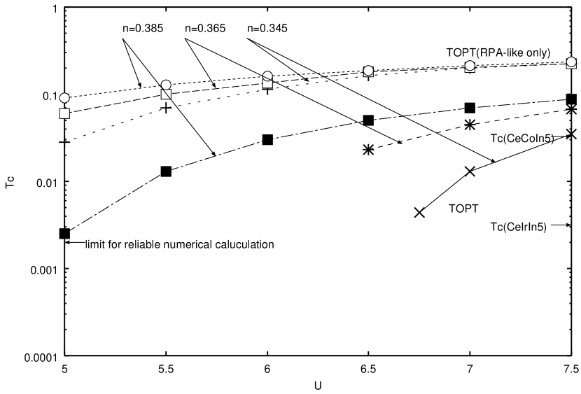
Figure 5: The calculated $T_{\rm c}$ as $U$ is varied and for various values of $n$ as shown in the figure. TOPT and TOPT(RPA-like only) in this figure mean that full diagrams and only RPA-like diagrams of anomalous self-energies up to third order are included, respectively.

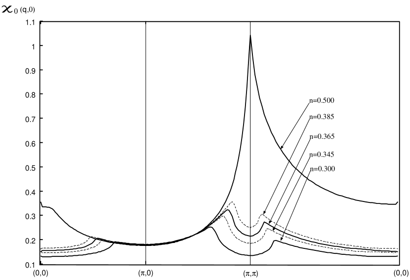
Figure 6: The momentum dependence of the static bare susceptibility for various $n$.

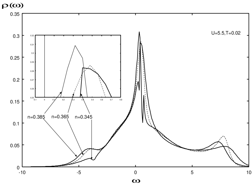
Figure 7: The density of states as $n$ is varied, at $U=5.5$ and $T=0.02$. The inset shows the details near the Fermi level.

The calculated gap functions show the node at $k_{x}=k_{y}$ and $k_{x}=-k_{y}$ and changes the sign across the node in all approximations and for all parameters. The symmetry of Cooper pair is $d_{x^{2}-y^{2}}$. The dependence of $T_{\rm c}$ on $U,n$ are shown in Fig. 5. To examine how the vertex corrections influence $T_{\rm c}$, we also calculate $T_{\rm c}$ by including only the RPA-like diagrams of anomalous self-energies up to third order, in other words, without the vertex corrections. We compare obtained $T_{\rm c}$(RPA-like only) with $T_{\rm c}$ calculated by including full diagrams of anomalous self-energies up to third order, in Fig. 5. From this figure, we can point out the following facts. For large $U$ higher $T_{\rm c}$ are obtained commonly for all cases. $T_{\rm c}$ calculated by including only the RPA-like diagrams of anomalous self-energies up to third order is higher than $T_{\rm c}$ calculated by including full diagrams of them. These results show that the main origin of the d-wave superconductivity is the momentum and frequency dependence of spin fluctuations given by the RPA-like terms. The vertex corrections reduce $T_{\rm c}$ by one order of magnitude. So the vertex corrections is important for obtaining reasonable $T_{\rm c}$ and for differentiating $n$-dependence of $T_{{\rm c}}$. When we fix the Coulomb repulsion $U$ and increase $n(0.345\sim 0.385)$, the system get close to the half-filling state ($n=0.5$). In this case, the momentum dependence of $\chi_{0}({\bf q},0)$ is slightly enhanced (see Fig. 6 shown later) and at the same time Fermi level gets close to the van Hove singularity (see Fig. 7 shown later), then higher $T_{\rm c}$ are obtained. If we assume $U_{{\rm CeIrIn_{5}}}\simeq U_{{\rm CeCoIn_{5}}}$, $T_{{\rm c}}$ of ${\rm CeIrIn_{5}}$ with $n=0.345$ is lower than that of ${\rm CeCoIn_{5}}$ with $n=0.385$ and this tendency is in good agreement with experimental results.

3.5.3 Behavior of $\chi_{0}({\bf q},0)$

The calculated results of the static bare susceptibility are shown in Fig. 6 for various values of $n$. From this figure, we point out the following facts. In the case of half-filling state, $\chi_{0}({\bf q},0)$ has commensurate peak at $(\pi,\pi)$. When we increase $n(0.3\sim 0.5)$, the system get close to the half-filling state and the peak and the momentum dependence of $\chi_{0}({\bf q},0)$ are enhanced. In the case of $n=0.345\sim 0.385$, $\chi_{0}({\bf q},0)$ has the incommensurate peak around $(\pi,\pi)$. This peak is not prominent but $\chi_{0}({\bf q},0)$ has sufficiently strong momentum dependence. These results mentioned above indicates the $d_{x^{2}-y^{2}}$ symmetry of the gap function.

3.5.4 Density of states

The density of states(DOS) is given by

$$\rho(\omega)=-\frac{1}{N\pi}\sum_{{\bf k}}{\rm Im}G^{R}({\bf k},\omega),$$ (22)

where

$$G^{R}({\bf k},\omega)=\left.G({\bf k},\epsilon_{n})\right|_{{\rm i}\epsilon_{n}\rightarrow\omega+{\rm i}\eta}.$$

We show the $n$-dependence of DOS in Fig. 7. From inset in this figure, we can see that the position of the van Hove singularity shifts upward from the Fermi level with decreasing $n$. This departure of the van Hove singularity from the Fermi level reduces the superconducting transition temperature $T_{{\rm c}}$.

3.5.5 Self-energy

The self-energy is given by

$$\Sigma_{n}^{R}({\bf k},\omega)=\left.\Sigma_{n}({\bf k},\epsilon_{n})\right|_{{\rm i}\epsilon_{n}\rightarrow\omega+{\rm i}\eta}.$$

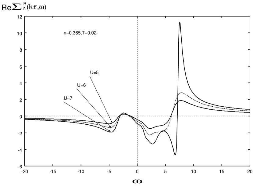
Figure 8: The real part of the normal self-energy at the Fermi momentum, at $n=0.365$, $T=0.02$ and for various values of $U$ as shown in the figure.

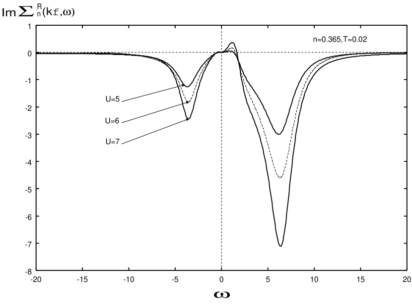
Figure 9: The imaginary part of the normal self-energy at the Fermi momentum, at $n=0.365$, $T=0.02$ and for various values of $U$ as shown in the figure.

The real part and the imaginary part of the self-energy at Fermi momentum are shown in Fig. 8 and Fig. 9 respectively. The $\omega$-dependence of both parts near $\omega=0$ are respectively given by ${\rm Re}\Sigma_{n}^{R}({\bf k}_{f},\omega)\propto-\omega$ and ${\rm Im}\Sigma_{n}^{R}({\bf k}_{f},\omega)\propto-\omega^{2}$. This behavior is the same as that for the usual Fermi liquid. As $U$ increases, the slope of ${\rm Re}\Sigma_{n}^{R}({\bf k}_{f},\omega)$ at $\omega=0$ becomes steeper and the coefficient of the $\omega^{2}$-term in ${\rm Im}\Sigma_{n}^{R}({\bf k}_{f},\omega)$ become larger. This indicates that the mass and the damping rate of the quasi-particle become larger as $U$ increases. These results are the typical Fermi liquid ones.

4 Summary, Discussion and Conclusion

In this paper, we have reformulated the superconducting transition on the quasi-particle description and discussed of the superconductivity of ${\rm CeIr}_{x}{\rm Co}_{1-x}{\rm In}_{5}$ on the basis of such a renormalized formula. By the low order perturbation expansion it is difficult to obtain actual mass enhancement factor. Here we have started from heavy fermions possessing a large effective mass. To obtain the anisotropic superconductivity we have taken account of the momentum dependence of interaction between quasi-particles. By this procedure we can make an argument consistent with both heavy electron mass and anisotropic superconductivity. Taking the importance of the most heavy quasi-two dimensional Fermi surface into account in realizing the superconductivity in ${\rm CeIr}_{x}{\rm Co}_{1-x}{\rm In}_{5}$, we have represented these bands with an effective single band two-dimensional Hubbard model and calculated $T_{\rm c}$ on the basis of the third order perturbation theory. We have pointed out that the main origin of their superconductivities can be ascribed to the momentum and frequency dependence of the spin fluctuations, although the vertex correction terms are important for reducing $T_{\rm c}$ then obtaining reasonable transition temperatures and differentiating $n$-dependence of $T_{{\rm c}}$.

Almost the same results have been obtained in the calculation of $T_{{\rm c}}$ for high-$T_{\rm c}$ cuprates performed by Hotta  [16] and for organic superconductors performed by Jujo et al.  [17], based on the third order perturbation theory. For high-$T_{\rm c}$ cuprates, Hotta calculated $T_{{\rm c}}$ on the basis of $d$-$p$ model and succeeded in reproducing experimentally obtained dependence of $T_{{\rm c}}$ on carrier number for overdoped cuprate within the third order perturbation theory. In spin-triplet superconductor ${\rm Sr_{2}RuO_{4}}$, Nomura and Yamada have recognized that the momentum and frequency dependence of the effective interaction between electrons which is not included in the interaction mediated by the spin fluctuation is essential for realizing the spin triplet pairing, by treating the electron correlation within the third order perturbation theory, on the basis of the two-dimensional single-band Hubbard model. [18]. According to their theory, third order vertex correction terms, which are not direct contribution from spin fluctuations, are important for the superconductivity in ${\rm Sr_{2}RuO_{4}}$. They also searched finite values of $T_{{\rm c}}$ within the second order perturbation theory (the second order term is the only term which is included in the interaction mediated by the spin fluctuation within the third order perturbation theory in the case of spin-triplet superconductivity of the single-band Hubbard model) and the random phase approximation, but could not find any finite value of $T_{{\rm c}}$ within the precision of their numerical calculations and for appropriate values of parameters. Recently Kondo has examined the superconductivity of the two-dimensional Hubbard model in the small $U$ limit within the second perturbation theory. One of his conclusion is also that the spin-triplet superconducting state is not stable in the small $U$ limit [19].

These facts described above suggest that the calculations of $T_{{\rm c}}$ which include only the spin fluctuation terms are questionable and should be carefully performed with other terms. In our calculation, the effects of other terms are taken into account by third order vertex correction terms which are not included in the interaction mediated by the spin fluctuation. We assume that the effect of the electron correlation is almost taken into account by the third order perturbation theory. To confirm this assumption, we have to do with the forth order perturbation theory. The forth order perturbation theory is a remaining future problem. We point out that in calculating the superconducting transition temperature $T_{{\rm c}}$ of typical heavy fermion superconductors, it is reasonable to treat the electron correlation by perturbation theory based on the Fermi liquid theory instead of taking only the effect of the specific diagrams which are favorable to the spin fluctuation.

The electronic structure of pressured ${\rm CeRhIn_{5}}(P>1.6{\rm GPa})$ is considered to be same structure of ${\rm CeCoIn_{5}}$. So we consider that the same mechanism can be applied to the mechanism of the superconductivity of pressured ${\rm CeRhIn_{5}}(P>1.6{\rm GPa})$.

In conclusion, we have reformulated the Éliashberg’s equation for the superconducting transition within the quasi-particle description which takes into account of the heavy electron mass. We also presented a microscopic mechanism for the d-wave superconductivity in ${\rm CeIr}_{x}{\rm Co}_{1-x}{\rm In}_{5}$ and attempted to explain the $x$-dependence of $T_{{\rm c}}$, by using such a renormalized formula and the perturbation theory.

Figure 1: The renormalized self-energy $\tilde{\Sigma}({\bf k},\omega)$ can be re-written as the expansion with respect to the quasi-particle Green’s function $\tilde{G}$ and the quasi-particle s-wave scattering interaction $\tilde{\Gamma}_{\rm loc}=a^{2}\Gamma_{{\rm loc}}$

Figure 2: The full vertex $\tilde{\Gamma}(1,2;3,4)$ can be re-written as the expansion with respect to the quasi-particle Green’s function $\tilde{G}$ and the quasi-particle s-wave scattering interaction $\tilde{\Gamma}_{\rm loc}=a^{2}\Gamma_{{\rm loc}}$

Figure 3: The Feynman diagrams of the normal self-energy up to third order. The solid and dashed lines correspond to the bare Green’s function and the interaction, respectively.

Figure 4: The Feynman diagrams of the effective interaction up to third order. The solid and dashed lines correspond to the bare Green’s function and the interaction, respectively. The diagrams enclosed by the dashed line are vertex corrections. The other diagrams are included in RPA.

References

- [1] F. J. Ohkawa: Phys. Rev. B 59 (1999) 8930.
- [2] A. M. Tsvelisk and P. B. Wiegmann: Ad. Physics 32 (1983) 453.
- [3] N. Kawakami and A. Okiji: Phys. Lett. 86A (1981) 483.
- [4] A. Okiji and N. Kawakami: J. Appl. Phys. 55 (1984) 1931.
- [5] V. Zlati and Horvati: Phys. Rev. B28 (1983) 6904.
- [6] K. Yamada and K. Yosida: Prog. Theor. Phys. 76 (1986) 621.
- [7] A. C. Hewson: Phys. Rev. Lett. 70 (1993) 4007.
- [8] A. C. Hewson: Ad. Phys. 43 (1994) 543.
- [9] C. Petrovic, R. Movshovich, M. Jaime, P. G. Pagliuso, M. F. Hundley, J. L. Sarrao, Z. Fisk and J. D. Thompson: Eur. Lett. 53 (3) (2001) 354.
- [10] C. Petrovic, P. G. Pagliuso, M. F. Hundley, R. Movshovich, J. L. Sarrao, J. D. Thompson, Z. Fisk and P. Monthoux: J. Phys-Condense Mat. 13 (17) (2001) L337 .
- [11] H. Hegger, C. Petrovic, E. G. Moshopoulou, M. F. Hundley, J. L. Sarro, Z. Fisk and J. D. Thompson: Phys. Rev. Lett. 84 (2001) 4986.
- [12] K. Izawa, H. Yamaguchi, Y. Matsuda, H. Shishido, R. Settai and nuki: Phys. Rev. Lett. 87 (2001) 057002.
- [13] P. G. Pagliuso, R. Movshovich, A. D. Bianchi, M. Nicklas, N. O. Moreno, J. D. Thompson, M. F. Hundley, J. L. Sarrao and Z. Fisk: cond-mat/0107266 v2.
-
[14]
Y. Haga, Y. Inada, H. Harima, K. Oikawa,
M. Murakawa, H. Nakawaki, Y. Tokiwa,
D. Aoki, H. Shishido, S. Ikeda, N. Watanabe, and Y. nuki: Phys. Rev. B 63 (2001) 060503. -
[15]
R. Settai, H. Shishido, S. Ikeda,
Y. Murakawa, H. Nakawaki, M. Nakashima,
D. Aoki, Y. Haga, H. Harima, and Y. nuki: J. Phys-Condense Mat. 13 (27)(2001) L627. - [16] T.Hotta: J. Phys. Soc. Jpn. 63 (1994) 4126.
- [17] T.Jujo, S.Koikegami and K.Yamada: J. Phys. Soc. Jpn. 68 (1999) 1331.
- [18] T.Nomura and K.Yamada: J. Phys. Soc. Jpn. 69 (2000) 3678.
- [19] J.Kondo: J. Phys. Soc. Jpn. 70 (2001) 808.