Perturbation Theory on the Superconductivity of Heavy Fermion Superconductor ${\rm UPd_{2}Al_{3}}$

Abstract

We investigate the superconducting mechanism and the transition temperature of heavy fermion superconductor ${\rm UPd_{2}Al_{3}}$ on the basis of a single band two-dimensional Hubbard model on triangular lattice, which represents the most heavy band of ${\rm UPd_{2}Al_{3}}$. Both normal and anomalous self-energies are calculated up to third order with respect to the Coulomb repulsion $U$ between itinerant electrons. The superconducting transition temperature is obtained by solving the ${\rm\acute{E}}$liashberg’s equation. Reasonable transition temperatures are obtained for moderately large $U$. It is found that the momentum and frequency dependence of spin fluctuations given by RPA-like terms gives rise to the d-wave pairing state, while the vertex correction terms are important for obtaining reasonable transition temperatures. These results seem to show that the superconductivity in ${\rm UPd_{2}Al_{3}}$ can be explained by the perturbation theory with respect to $U$.

1 Introduction

1.1 Introduction to ${\rm UPd_{2}Al_{3}}$

${\rm UPd_{2}Al_{3}}$ crystallizes in the hexagonal ${\rm PrNi_{2}Al_{3}}$-type structure and it was found to be a superconductor with $T_{\rm c}=$2K. The superconducting state coexists with antiferromagnetic order below the N${\rm\acute{e}}$el temperature $T_{\rm N}$=14.5K [1]. The magnetic moments are aligned ferromagnetically in the hexagonal basal plane and coupled antiferromagnetically between planes with wave vector ${\bf k}=[0,0,0.5]$ [2].

For $T\leq T_{\rm N}$, the electrons in ${\rm UPd_{2}Al_{3}}$ behave as if they were separated into two rather independent subsystems of 5f character [3, 4]. One subsystem is a localized system which is responsible for antiferromagnetic order. We call this system “localized subsystem”. The second subsystem is the itinerant one characterized as a heavy electron system and responsible for the superconductivity. We call the latter “itinerant subsystem”. For $T_{\rm c}<T\ll T_{\rm N}$ in the normal state, the electronic specific-heat $C$ can be approximated by $C\simeq\gamma T$ where $\gamma=145$mJ/${\rm K}^{2}$ [1]. For $T_{\rm c}<T<$4K in the normal state, the electrical resistivity curve follows the dependence $\rho=\rho_{0}+AT^{2}$ where $\rho_{0}=2.3{\rm\mu\Omega cm}$ and $A\simeq 10^{-1}{\rm\mu\Omega cm/K^{2}}$ [5]. The behavior observed in the electronic specific-heat and the electrical resistivity indicates that the itinerant electrons in ${\rm UPd_{2}Al_{3}}$ compose a Fermi liquid.

The calculated Fermi surface in the antiferromagnetic state has four principal sheets of predominately $f-$electron character [6, 7, 8, 9]. These are corroborated by de Haas-van Alphen measurements [8]. All bands are doubly degenerated, because the antiferromagnetic structure is conserved under a time-reversal and inversion-symmetry operator with the non-primitive translation vector ${\bf v}=(0,0,0.5)$. The Fermi sheets are not of hexagonal symmetry, reflecting the antiferromagnetic structure. Roughly speaking, two Fermi sheets have two-dimensional topology, and the remaining two Fermi sheets have the dispersion along the crystallographic $c-$axis, although there exist some discrepancies between the results of ref.rf:band2 and ref.rf:band3ref . In ref.rf:band2, two Fermi sheets which have two-dimensional topology are called , “party hat” and ”cylinder”, and the remaining two are called “cigar” and ”eggs”. According to the band calculation and de Haas-van Alphen measurements [8], the band which has the largest effective mass is “party hat”.

As for the superconducting property, the specific heat and the nuclear spin-lattice relaxation rate $T_{1}$ show the $T^{3}$- dependence without the coherence peak just below $T_{\rm c}$ [10, 11, 12]. The Knight shifts decrease below $T_{\rm c}$ [10]. The thermal conductivity $\kappa$ dose not show any anomaly at $T_{\rm c}$ and shows the $T^{2}$ behavior below 1K [5]. These facts suggest that the superconductivity is in principle of a d-wave type characterized by vanishing gaps on the lines on the Fermi surface, although there exist some discrepancies between the results of the specific heat and NMR. Inelastic neutron scattering  [13, 14, 15, 16, 17, 18] and tunneling experiments [19, 20] below the superconducting transition temperature have been performed on this material. The results of these experiments indicate that superconductivity and magnetic excitations of antiferromagnetically ordered moments in ${\rm UPd_{2}Al_{3}}$ couple each other.

1.2 Motivation

Itinerant electrons in heavy fermion systems compose a Fermi liquid whose effective mass is enhanced by $10^{2}\sim 10^{3}$ times as large as that of free electron. The electron correlation is essential in giving the large electron mass in heavy electron systems. From this point of view, we can expect that superconductivities in heavy fermion systems are derived also from the electron correlation through the momentum and frequency dependence of the effective interaction between electrons. In fact, in other strongly correlated electron systems such as high-$T_{\rm c}$ cuprates [21], organic superconductors [22] and spin-triplet superconductor ${\rm Sr_{2}RuO_{4}}$ [23], it has been recognized that the electron correlation plays an important role in realizing their superconductivities, by treating the electron correlation by perturbation theory based on Fermi liquid theory.

As described above, recent neutron scattering experiments done below $T_{\rm c}$ revealed a strong relationship between the superconductivity and magnetic excitations of antiferromagnetically ordered moments in ${\rm UPd_{2}Al_{3}}$. Indicated by these experimental facts, several groups [24, 25, 26] have proposed a new mechanism mediated by spin wave in the ordered antiferromagnetic state. This mechanism is called “magnetic exciton” mechanism. Magnetic excitons are a kind of spin waves that ripple through a magnetically ordered medium, but they require a certain amount of energy to be excited. They argued that these magnetic excitons may produce an effective interaction between the itinerant electrons, and so be responsible for superconductivity in a manner analogous to that played by phonons in conventional superconductors. Therefore, for “magnetic exciton” mechanism, the coupling between the “localized subsystem”and the “itinerant subsystem” is essential to deriving the superconductivity.

The proposal seems to be interesting as a new mechanism. However, it is not clear whether this mechanism can actually realize the superconductivity or not, since there is no quantitative calculation of the critical temperature $T_{\rm c}$. To the present authors, it seems to be natural that the largest Fermi sheet with large electron mass itself leads to the superconductivity by a mechanism due to the effective interaction between electrons in the “itinerant subsystem”.

In this paper, we investigate the possibility that the superconductivity in ${\rm UPd_{2}Al_{3}}$ is derived from the electron correlation effects existing in “itinerant subsystem”, by the perturbation theory with respect to Coulomb repulsion $U$. We show that the superconductivity in ${\rm UPd_{2}Al_{3}}$ can be explained by the usual spin fluctuation mechanism in the “itinerant subsystem”. This explanation will be given on the basis of detailed calculation where the dependence on the parameters inherent in ${\rm UPd_{2}Al_{3}}$ are carefully studied. We concentrate our attention on the calculation of the superconducting transition temperature $T_{{\rm c}}$, so we do not investigate the relationship between superconductivity and magnetic excitation of antiferromagnetically ordered moments in ${\rm UPd_{2}Al_{3}}$ far below $T_{{\rm c}}$, in this paper.

The organization of this paper is as follows. In $\S 2$ formulation is presented, including model Hamiltonian, perturbation expansion terms and ${\rm\acute{E}}$liashberg’s equation. In $\S 3$ calculation results of $T_{\rm c}$ and other various quantities are shown. Finally in $\S 4$ discussions and conclusion are presented.

2 Formulation

2.1 Model and Hamiltonian

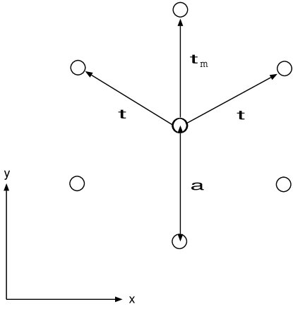
Figure 1: Schematic figure of the hexagonal basal plane of ${\rm UPd_{2}Al_{3}}$. Circles in this figure represent U atoms.

Taking the importance of the correlation between electrons in the “itinerant subsystem” into account in realizing the d-wave superconductivity, we consider only a single band of ${\rm UPd_{2}Al_{3}}$ possessing the largest effective mass. According to the band calculation [8], the band of ${\rm UPd_{2}Al_{3}}$ possessing the largest effective mass (which is the so called “party hat”) has the property of quasi-two-dimensional. Therefore we represent the band as a simple effective two-dimensional Hubbard model on the triangular lattice. We set $x$-$y$ plane in the hexagonal basal plane, and set $y$-axis parallel to antiferromagnetic moments. We consider only the nearest neighbor hopping integrals and we assume for the $y$-direction hopping integral a different value $t_{\rm m}$ from other hopping integrals $t$, because the superconductivity of ${\rm UPd_{2}Al_{3}}$ is realized in the antiferromagnetic state [2](see Fig. 1). So we consider that the effect of the antiferromagnetic order(the effect of the “localized subsystem”) is included in the difference between $t_{\rm m}$ and $t$, and we determine the values so as to reproduce the considered Fermi sheet which is obtained by the band calculation and is not of hexagonal symmetry, reflecting the antiferromagnetic structure(“localized subsystem”).

We rescale length, energy, temperature, time by $a,t,\frac{t}{k_{\rm B}},\frac{\hbar}{t}$ respectively (where $a,k_{\rm B},\hbar$ are the lattice constant of the hexagonal basal plane, Boltzmann constant, Planck constant divided by $2\pi$ respectively), we write our model Hamiltonian as follows:

$$H = H_{0}+H_{1},$$ (1)

$$H_{0} = \sum_{{\bf k},\sigma}\left(\epsilon({\bf k})-\mu\right)a_{{\bf k}\sigma}^{\dagger}a_{{\bf k}\sigma},$$ (2)

$$\epsilon({\bf k})=-4\cos(\frac{\sqrt{3}}{2}k_{x})\cos(\frac{1}{2}k_{y})-2t_{\rm m}\cos(k_{y}),$$ (3)

$$H_{1}=\frac{U}{2N}\sum_{\sigma\neq\sigma^{\prime}}\sum_{{\bf k}_{1}{\bf k}_{2}{\bf k}_{3}{\bf k}_{4}}\delta_{{\bf k}_{1}+{\bf k}_{2},{\bf k}_{3}+{\bf k}_{4}}a_{{\bf k}_{1}\sigma}^{\dagger}a_{{\bf k}_{2}\sigma^{\prime}}^{\dagger}a_{{\bf k}_{3}\sigma^{\prime}}a_{{\bf k}_{4}\sigma},$$ (4)

where $a_{{\bf k}\sigma}^{\dagger}(a_{{\bf k}\sigma})$ is the creation(annihilation) operator for the electron with momentum ${\bf k}$ and spin index $\sigma$; $t_{\rm m}$ and $\mu$ are the $y$-direction hopping integral and the chemical potential, respectively. The sum over ${\bf k}$ indicates taking summation over a primitive cell of the inverse lattice. We set this primitive cell of the inverse lattice as shown in Fig. LABEL:fig:invlat for the convenience of our numerical calculation.

2.1.1 model parameters

Our model parameters are temperature $T$, $y$-direction hopping integral $t_{\rm m}$, the Coulomb repulsion $U$ and the electron number $n$ per one spin site. The bare bandwidth $\Delta\epsilon(t_{\rm m})$ of our model is

$$\Delta\epsilon(t_{\rm m})=\left\{\begin{array}[]{@{\,}ll}8&\mbox{($0<t_{\rm m}<0.5$)}.\\ 4+4t_{\rm m}+1/t_{\rm m}&\mbox{($t_{\rm m}\geq 0.5$)}.\end{array}\right.$$ (5)

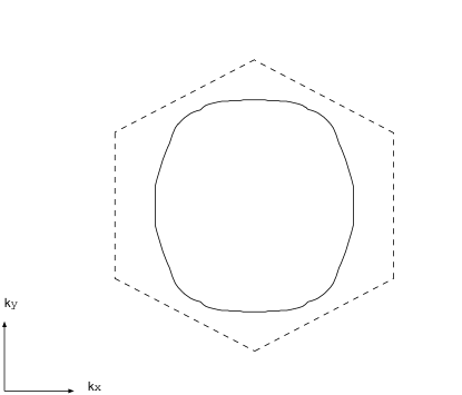
Figure 3: The bare Fermi surface calculated by our model. The region enclosed by the dashed line is the first Brillouin zone. See also Fig.5(b) in ref.  rf:band3ref.

According to the band calculation and the de Haas-van Alphen experiment [8],the parameter region of our model which reproduces the Fermi sheet is given by $0.50\leq t_{\rm m}\leq 0.75$ and $0.51\leq n\leq 0.572.$ In this parameter region, the range of the bare bandwidth is $8\leq\Delta\epsilon(t_{\rm m})\leq 8.333\cdots$. We consider that $t_{\rm m}=0.75,n=0.572$ are the best fitting values of parameters which well reproduce the Fermi sheet we consider. In Fig. 3, the bare Fermi surface calculated by our model (the model parameters are $t_{\rm m}=0.75,n=0.572,U=0$ and $T=0$) is presented. From this figure we can see that the considered Fermi sheet determined by the band calculation [8] is well reproduced within our effective model.

The superconducting transition temperature determined by experiments is about 2K [1].Then the rescaled superconducting transition temperature $T_{\rm c}$ is $T_{\rm c}\simeq 1.4\times 10^{-3}$, when we set $1$eV as the value of bandwidth obtained by the band calculation [8, 9].

2.2 Green’s functions

2.2.1 Bare Green’s functions

The bare Green’s function is the following,

$$G^{(0)}(k)=\frac{1}{{\rm i}\epsilon_{n}-\epsilon({\bf k})+\mu},$$ (6)

where $\epsilon_{n}=(2n+1)\pi T(n:{\rm integer})$ is the fermion-Matsubara frequency and short notation $k=({\bf k},\epsilon_{n})$ is adopted. We consider the Hartree term is included in the chemical potential.

2.2.2 Dressed normal Green’s functions

Next we consider the dressed normal Green’s function. When we consider the situation near the superconducting transition temperature, the Dyson-Gorkov’s equation can be linearized. Therefore the dressed normal Green’s function is obtained from the bare Green’s function with only the normal self-energy correction. We expand the normal self-energy up to third order with respect to $U$;the diagrams are shown in Fig. 4.

Then we obtain the normal self-energy as follows,

$$\Sigma_{n}(k)=\frac{T}{N}\sum_{k^{\prime}}[U^{2}\chi_{0}(k-k^{\prime})+U^{3}\chi_{0}^{2}(k-k^{\prime})+U^{3}\phi_{0}^{2}(k+k^{\prime})]G_{0}(k^{\prime}),$$ (7)

where $\chi_{0}(\cdots)$ and $\phi_{0}(\cdots)$ are given respectively as

$$\chi_{0}({\bf q},\omega_{m})=-\frac{T}{N}\sum_{{\bf k},n}G_{0}({\bf k},\epsilon_{n})G_{0}({\bf q}+{\bf k},\omega_{m}+\epsilon_{n}),$$ (8)

$$\phi_{0}({\bf q},\omega_{m})=-\frac{T}{N}\sum_{{\bf k},n}G_{0}({\bf k},\epsilon_{n})G_{0}({\bf q}-{\bf k},\omega_{m}-\epsilon_{n}).$$ (9)

Here $\omega_{m}=2m\pi T(m:{\rm integer})$ is the boson-Matsubara frequency. The quantity $\chi_{0}({\bf q},\omega_{m})$ has the physical meaning of the bare susceptibility and expresses spin fluctuations in the system. More over, the bare susceptibility plays an important role in the calculation of $T_{\rm c}$, that is, it determines the magnitude and the spatial and temporal variation of the effective interaction between electrons in the “itinerant subsystem”, through the higher order terms in $U$. (See the first term of right hand side of the equation 2.13.)

Note that the Hartree term has been already included in the chemical potential and the constant terms which have not been included in the Hartree term are included in the chemical potential shift when we fix the particle number.

Then the dressed normal Green’s function is

$$G(k)=\frac{1}{{\rm i}\epsilon_{n}-(\epsilon({\bf k})-\mu-\delta\mu+\Sigma_{n}(k))},$$ (10)

where $\delta\mu$ is determined so that the following equation is satisfied.

$$n=\frac{T}{N}\sum_{k}G(k)=\frac{T}{N}\sum_{k}G_{0}(k).$$ (11)

We expand the above equation up to the third order of the interaction with regard to $\delta\mu-\Sigma_{n}(k)$, we obtained $\delta\mu$ as

$$\delta\mu=-\frac{\frac{T}{N}\sum_{k}G_{0}^{2}(k)\Sigma_{n}(k)}{\chi_{0}({\bf 0},0)}.$$ (12)

2.2.3 Anomalous self-energy and effective interaction

When we consider the situation near the superconducting transition temperature, the anomalous self-energy $\Sigma_{a}(k)$ is represented by the anomalous Green’s function $F(k)$ and the (normal)effective interaction. We expand the effective interaction up to third order with respect to $U$ as shown in Fig. 5.

Then we obtain the anomalous self-energy as follows;

$$\Sigma_{a}(k) = -\frac{T}{N}\sum_{k^{\prime}}[U+U^{2}\chi_{0}(k+k^{\prime})+2U^{3}\chi_{0}^{2}(k+k^{\prime})]F(k^{\prime})$$ (13)

$$\mbox{}-U^{3}\frac{T^{2}}{N^{2}}\sum_{k^{\prime}k^{\prime\prime}}G_{0}(k^{\prime})[\chi_{0}(k+k^{\prime})-\phi_{0}(k+k^{\prime})]G_{0}(k+k^{\prime}-k^{\prime\prime})F(k^{\prime\prime})$$

$$\mbox{}-U^{3}\frac{T^{2}}{N^{2}}\sum_{k^{\prime}k^{\prime\prime}}G_{0}(k^{\prime})[\chi_{0}(-k+k^{\prime})-\phi_{0}(-k+k^{\prime})]G_{0}(-k+k^{\prime}-k^{\prime\prime})F(k^{\prime\prime}).$$

2.3 $\acute{E}$liashberg’s equation

From the linearized Dyson-Gorkov equation, we obtain the anomalous Green’s function as follows;

$$F(k)=|G(k)|^{2}\Sigma_{a}(k).$$ (14)

Then the ${\rm\acute{E}liashberg}$’s equation is given by

$$\Sigma_{a}(k) = -\frac{T}{N}\sum_{k^{\prime}}[U+U^{2}\chi_{0}(k+k^{\prime})+2U^{3}\chi_{0}^{2}(k+k^{\prime})]|G(k^{\prime})|^{2}\Sigma_{a}(k^{\prime})$$

$$\mbox{}-U^{3}\frac{T^{2}}{N^{2}}\sum_{k^{\prime}k^{\prime\prime}}G_{0}(k^{\prime})[\chi_{0}(k+k^{\prime})-\phi_{0}(k+k^{\prime})]G_{0}(k+k^{\prime}-k^{\prime\prime})|G(k^{\prime\prime})|^{2}\Sigma_{a}(k^{\prime\prime})$$

$$\mbox{}-U^{3}\frac{T^{2}}{N^{2}}\sum_{k^{\prime}k^{\prime\prime}}G_{0}(k^{\prime})[\chi_{0}(-k+k^{\prime})-\phi_{0}(-k+k^{\prime})]G_{0}(-k+k^{\prime}-k^{\prime\prime})|G(k^{\prime\prime})|^{2}\Sigma_{a}(k^{\prime\prime}).$$

We consider that the system is superconducting state when the eigen value of this equation is 1.

3 Calculation Results

3.1 Details of the numerical calculation

To solve the ${\rm\acute{E}}$liahberg’s equation by using the power method algorithm, we have to calculate the summation over the momentum and the frequency space. Since all summations are in the convolution forms, we can carry out them by using the algorithm of the Fast Fourier Transformation. For the frequency, irrespective of the temperature, we have 1024 Matsubara frequencies. Therefore we calculate throughout in the temperature region $T\geq T_{\rm lim}$ , where $T_{\rm lim}$ is the lower limit temperature for reliable numerical calculation, which is estimated about $2.0\times 10^{-3}(>\Delta\epsilon(t_{\rm m})/(2\pi\times 1024)\simeq 1.3\times 10^{-3})$; we divide a primitive cell into 128$\times$128 meshes.

We have carried out analytically continuing procedure by using Pad${\rm\acute{e}}$ approximation.

3.2 Dependence of $T_{\rm c}$ on $U,t_{\rm m}$ and $n$

To solve the ${\rm\acute{E}}$liashberg’s equation, we set the initial gap function($d_{xy}$-symmetry) as follows.

$$\Sigma_{a}(k)\propto\sin\frac{\sqrt{3}}{2}k_{x}\sin\frac{1}{2}k_{y}.$$ (16)

Notice that the “itinerant subsystem” has no hexagonal symmetry due to the antiferromagnetic structure(“localized subsystem”). The calculated gap functions show the node at $k_{x}=0$ and $k_{y}=0$ and changes the sign across the node for all parameters. The symmetry of Cooper pair is $d_{xy}$.

We calculate $T_{\rm c}$ around the best fitting values of parameters($t_{\rm m}=0.75,n=0.572$) because the best fitting values of parameters have some arbitrariness.

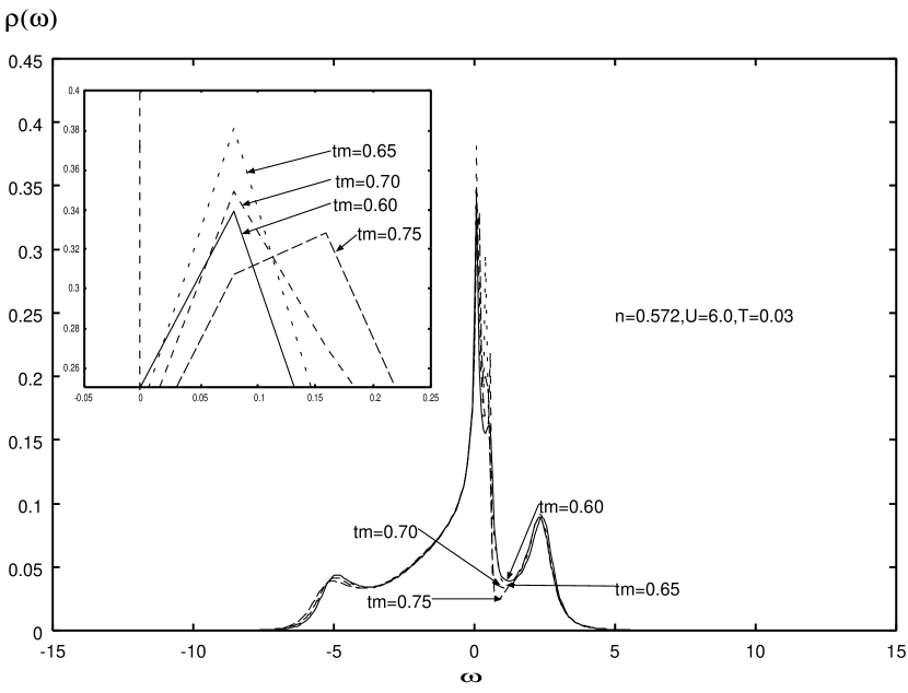
Figure 14: The density of states as $t_{\rm m}$ is varied, at $n=0.572$, $U=6.0$ and $T=0.03$. The inset shows the details near the Fermi level.

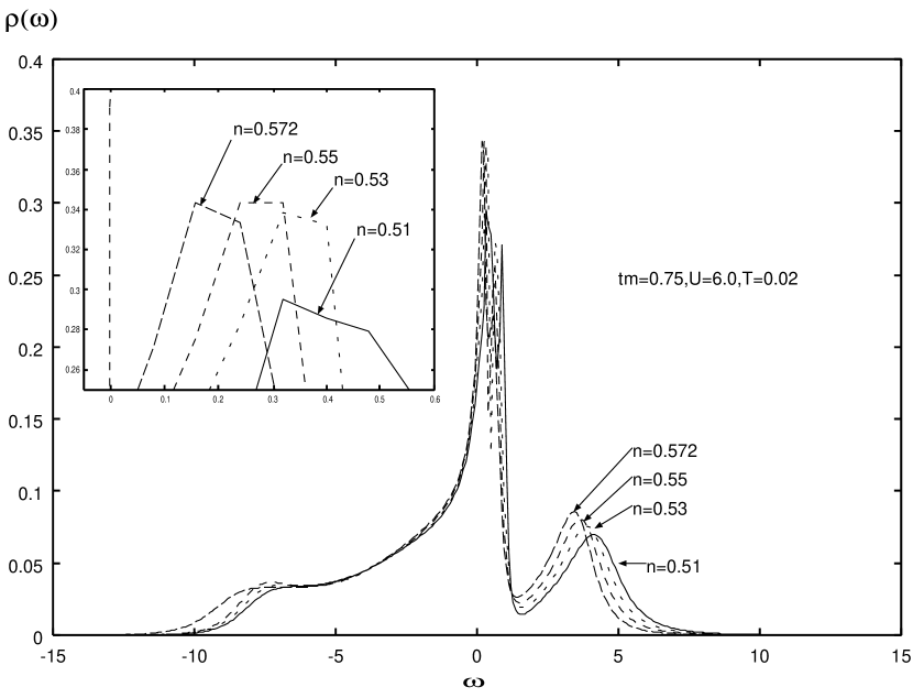
Figure 15: The density of states as $n$ is varied,at $t_{\rm m}=0.75$, $U=6.0$ and $T=0.02$. The inset shows the details near the Fermi level.

The dependence of $T_{\rm c}$ on $U,n$ and $t_{\rm m}$ are shown in Figs. LABEL:fig:n0.572Tc$\sim$ 9. From these results, we can point out the following facts. For large $U$ higher $T_{\rm c}$ are obtained commonly for all parameters. When we fix the electron number $n$ per one spin site and the Coulomb repulsion $U$, for large $t_{\rm m}$, the system get close to real triangular lattice ($t_{{\rm m}}=1$) for electrons in the “itinerant subsystem” and at the same time Fermi level goes away from the van Hove singularity(see Fig. 14 shown later), then lower $T_{\rm c}$ are obtained. Contrary, when we fix the $y-$direction hopping integral $t_{\rm m}$ and the Coulomb repulsion $U$, for large $n$, the system becomes away from the half-filling state ($n=0.5$) and at the same time Fermi level gets close to the van Hove singularity(see Fig. 15 shown later), then higher $T_{\rm c}$ are obtained.

3.3 Vertex corrections

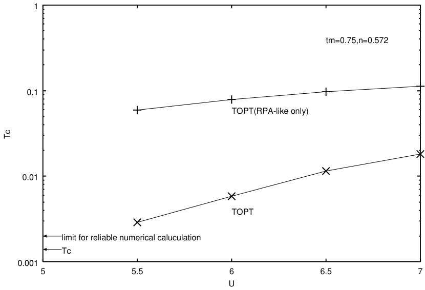
Figure 10: The calculated $T_{\rm c}$. TOPT and TOPT(RPA-like only) in this figure mean that full diagrams and only RPA-like diagrams of anomalous self-energies up to third order are included, respectively. See also Fig. 4.

To examine how the vertex corrections influence $T_{\rm c}$, we calculate $T_{\rm c}$ by including only RPA-like diagrams of anomalous self-energies up to third order, in other words, without the vertex corrections and compare obtained $T_{\rm c}$ with $T_{\rm c}$ calculated by including full diagrams of anomalous self-energies up to third order(Fig. 10). From this figure, we can see that $T_{\rm c}$ calculated by including only RPA-like diagrams of anomalous self-energies up to third order is higher than $T_{\rm c}$ calculated by including full diagrams of them. This figure shows that the main origin of the d-wave superconductivity is the momentum and frequency dependence of spin fluctuations given by the RPA-like terms; spin fluctuations exist in our nested Fermi sheet, and the Coulomb interaction among electrons in “itinerant subsystem”. The vertex corrections reduce $T_{\rm c}$ by one order of magnitude. So the vertex corrections is important for obtaining reasonable $T_{\rm c}$.

3.4 Behavior of $\chi_{0}(q)$

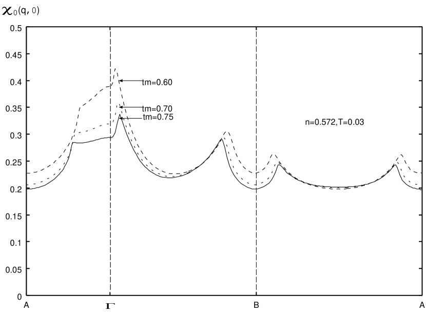
Figure 11: The momentum dependence of the static bare susceptibility for various $t_{\rm m}$. The notations under the horizontal axis are defined in Fig.2. These results are obtained for $n=0.572$, $T=0.03$.

The calculated results of the static bare susceptibility are shown in Fig. 11$\sim$ 13 for various value of $t_{\rm m}$ and $n$. From these figures, we point out the following facts. For all parameters, $\chi_{0}({\bf q},0)$ have sufficiently strong momentum dependence, although there exist no prominent peak. When we fix the electron number $n$ per one spin site and increase the parameter $t_{\rm m}$, the system approaches the real triangular lattice for electrons in the “itinerant subsystem”. In this case the peak and the momentum dependence of $\chi_{0}({\bf q},0)$ is slightly suppressed since the antiferromagnetic spin fluctuations are suppressed by the frustration effect in triangular lattice. Contrary, when we fix the $y-$direction hopping integral $t_{\rm m}$ and increase the electron number $n$ per one spin site, the system become away from the half-filling state and the peak and the momentum dependence of $\chi_{0}({\bf q},0)$ is slightly enhanced. The reason is that Fermi surface possesses some nesting properties with increasing $n$ from half-filling case, where the Fermi surface is similar to a circle without nesting properties.

3.5 Density of states

The density of states(DOS) is given by

$$\rho(\omega)=-\frac{1}{N\pi}\sum_{{\bf k}}{\rm Im}G^{R}({\bf k},\omega),$$ (17)

where

$$G^{R}({\bf k},\omega)=\left.G({\bf k},\epsilon_{n})\right|_{{\rm i}\epsilon_{n}\rightarrow\omega+{\rm i}\eta}.$$

We show the $t_{\rm m}$ and $n$- dependence of DOS in Figs. 14 and  15. From insets in these figures, we can see that the position of the van Hove singularity shifts upward from the Fermi level with increasing $t_{{\rm m}}$ and decreasing $n$. This departure of the van Hove singularity from the Fermi level reduces the superconducting transition temperature $T_{{\rm c}}$.

3.6 Self-energy

The self-energy is given by

$$\Sigma_{n}^{R}({\bf k},\omega)=\left.\Sigma_{n}({\bf k},\epsilon_{n})\right|_{{\rm i}\epsilon_{n}\rightarrow\omega+{\rm i}\eta}.$$

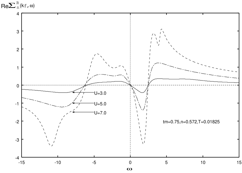
Figure 16: The real part of the normal self-energy at the Fermi momentum, at $t_{\rm m}=0.75$, $n=0.572$, $T=0.01825$ and for various values of $U$ as shown in the figure.

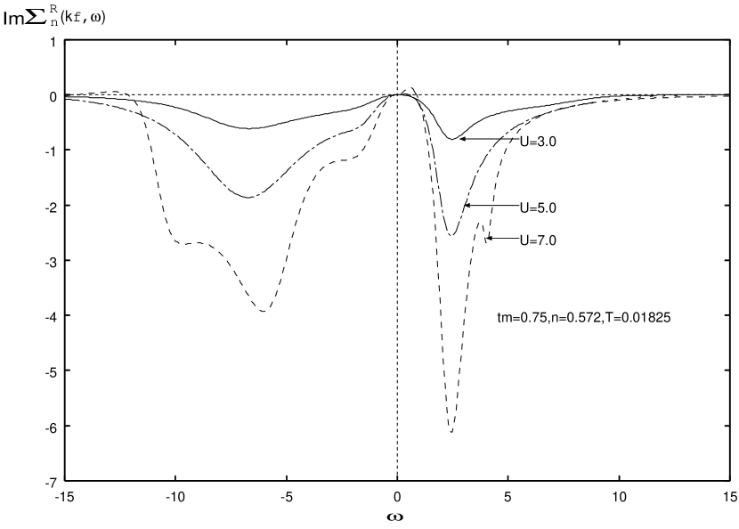
Figure 17: The imaginary part of the normal self-energy at the Fermi momentum, at $t_{\rm m}=0.75$, $n=0.572$, $T=0.01825$ and for various values of $U$ as shown in the figure.

The real part and the imaginary part of the self-energy at Fermi momentum are shown in Fig. 16 and Fig. 17 respectively. The $\omega$-dependence of both parts near $\omega=0$ are respectively given by ${\rm Re}\Sigma_{n}^{R}({\bf k}_{f},\omega)\propto-\omega$ and ${\rm Im}\Sigma_{n}^{R}({\bf k}_{f},\omega)\propto-\omega^{2}$. This behavior is the same as that for the usual Fermi liquid. As $U$ increases, the slope of ${\rm Re}\Sigma_{n}^{R}({\bf k}_{f},\omega)$ at $\omega=0$ becomes steeper and the coefficient of the $\omega^{2}$-term in ${\rm Im}\Sigma_{n}^{R}({\bf k}_{f},\omega)$ become larger. This indicates that the mass and the damping rate of the quasi-particle become larger as $U$ increases. These results are the typical Fermi liquid ones.

4 Summary, Discussion and Conclusion

In this paper, taking the importance of the correlation effect between electrons in “itinerant subsystem” into account in realizing the superconductivity, we have considered a single band of ${\rm UPd_{2}Al_{3}}$ whose effective mass is the largest. We have represented the band with an effective two-dimensional Hubbard model on triangular lattice and calculated $T_{\rm c}$ on the basis of third order perturbation theory. Reasonable transition temperatures have been obtained for moderately large $U$. We also have calculated $T_{\rm c}$ by including only RPA-like diagrams of anomalous self-energies up to third order, in other words, without the vertex corrections and compared it with $T_{\rm c}$ calculated by including full diagrams of anomalous self-energies up to third order. We point out that the main origin of the superconductivity can be ascribed to the momentum and frequency dependence of the spin fluctuations and the correlation between electrons in the “itinerant subsystem”, although the vertex correction terms are important for reducing $T_{\rm c}$ and obtaining reasonable transition temperatures. We have calculated DOS and the normal self-energy. The obtained behavior of both quantities is the expected one for the Fermi liquid.

Now, we briefly discuss the theories suggesting that the superconductivity in ${\rm UPd_{2}Al_{3}}$ is derived from the mechanism of exchanging “magnetic excitons”. Huth et al. [24] predicted that line nodes are at the rim of the magnetic Brillouin zone and on the “cigar” Fermi sheet. Their theory is based on the assumption of the pairing interaction mediated by the exchanging “magnetic excitons” and the band structure calculated by K.Kn${\rm\ddot{o}pfle}$ et al. [7]. Miyake and Sato [25] also predicted that the line node is on the plane very close to the zone boundary of the folded Brillouin zone in the antiferromagnetically ordered state on the basis of the itinerant-localized duality model; their theory is also based on the observed behavior of the dynamical magnetic susceptibility and the assumption of the pairing interaction induced by the exchanging “magnetic excitons” but without using any information about the Fermi sheets. According to these analysis [24, 25], Fermi sheets which have the dispersion along the crystallographic c-axis and cross the zone boundary plane of the folded Brillouin zone in the antiferromagnetically ordered state are necessary to possess the line nodes actually. On the other hand, according to the band calculation performed by Inada et al. [8], the “cigar” Fermi sheet dose not cross the zone boundary plane of the folded Brillouin zone in the antiferromagnetically ordered state, while the “cigar” Fermi sheet calculated by Kn${\rm\ddot{o}pfle}$ et al. [7] crosses this plane. Moreover, Inada et al. [8, 27] have tried to determine the position of the line node on the actual Fermi surface by the de Haas-van Alphen experiment. Their conclusion is that any line node in the anisotropic energy gap does not exist on the “cigar” Fermi sheet and/or it is difficult to distinguish experimentally the line node from the gapless state created by the pair-breaking effects by the applied magnetic field. Therefore, we now consider that the basis of “magnetic exciton” mechanism has not been confirmed.

These theories described above are indicated by the existence of the coupling between the superconductivity and the magnetic excitations of antiferromagnetically ordered moments in ${\rm UPd_{2}Al_{3}}$ below $T_{\rm c}$. Generally speaking, the coupling between superconductivity and magnetism exists more or less. Therefore it doesn’t always follow that superconductivity is mainly derived from the magnetic mechanism by the reason why there exists the coupling between superconductivity and magnetism. This is understood from the fact that the coupling between superconductivity and spin fluctuations or phonons is detected in high-$T_{\rm c}$ superconductors but the superconductivities in high-$T_{\rm c}$ are not always mainly derived from these spin fluctuations or phonons.

On the other hand, above $T_{\rm c}$, the behavior of the electronic specific-heat and the electrical resistivity are the typical Fermi liquid ones and anomalous behavior of these quantities is not detected in ${\rm UPd_{2}Al_{3}}$ ,for example, such as $\rho-\rho_{0}\propto T$ in high $T_{\rm c}$ superconductor. Moreover the magnetic transition temperature($T_{\rm N}=14$K) is sufficiently higher than the superconducting transition temperature($T_{\rm c}=2$K). Therefore we consider that the coupling between local moments (“localized subsystem”) and electrons in the “itinerant subsystem” is not so strong, while Sato et al. assume that this coupling is very strong in ref.rf:SM.

Therefore we considered that the electron correlation in the “itinerant subsystem” also plays an important role to derive the superconductivity in ${\rm UPd_{2}Al_{3}}$. Quasi-two-dimensional Fermi sheet so called “party hat” is most favorable to superconductivity, because of the most strong electron correlation in the “itinerant subsystem”. Our proposition is that this sheet possessing large area and electron mass is essential to derive the superconductivity in ${\rm UPd_{2}Al_{3}}$, while the Fermi sheets called “cigar”and “eggs”playing an essential role in realizing the superconductivity mediated by “magnetic exciton” seem to be too small to induce the superconductivity in the total system.

In the last, we also point out that results of tunneling experiments and our proposition don’t contradict. Tunneling spectra have been also measured in this material by the same group [19, 20]. Their conclusion is that an energy gap along the c-axis in ${\rm UPd_{2}Al_{3}}$ is well resolved. In the multi band system such an ${\rm UPd_{2}Al_{3}}$, the superconducting transition, in principle, simultaneously occurs in all Fermi sheets. Therefore the energy gaps open in all Fermi sheets below $T_{\rm c}$, then an energy gap along the c-axis exists in ${\rm UPd_{2}Al_{3}}$ since ${\rm UPd_{2}Al_{3}}$ is not a perfect two-dimensional system.

In conclusion we present a new mechanism that the superconductivity in ${\rm UPd_{2}Al_{3}}$ can be also derived from the correlation between electrons in the “itinerant subsystem” and the symmetry of the pairing state is $d_{xy}$. In our model, the main origin of the superconductivity is the momentum and frequency dependence of the spin fluctuations and the Coulomb interaction between electrons in the “itinerant subsystem”. This momentum and frequency dependence of the spin fluctuations stems from the shape of our Fermi sheet which undergoes the symmetry-breakdown due to the antiferromagnetic order(“localized system”) and then possesses nesting properties.

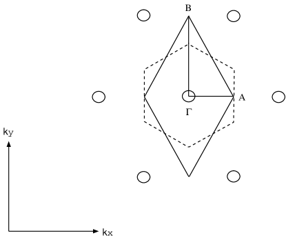
Figure 2: Our primitive cell of the inverse lattice. The regions enclosed by the solid and dashed lines are our primitive cell and the first Brillouin zone, respectively.

Figure 4: The Feynman diagrams of the normal self-energy up to third order. The solid and dashed lines correspond to the bare Green’s function and the interaction, respectively.

Figure 5: The Feynman diagrams of the effective interaction up to third order. The solid and dashed lines correspond to the bare Green’s function and the interaction, respectively. The diagrams enclosed by the dashed line are vertex corrections. The other diagrams are included in RPA.

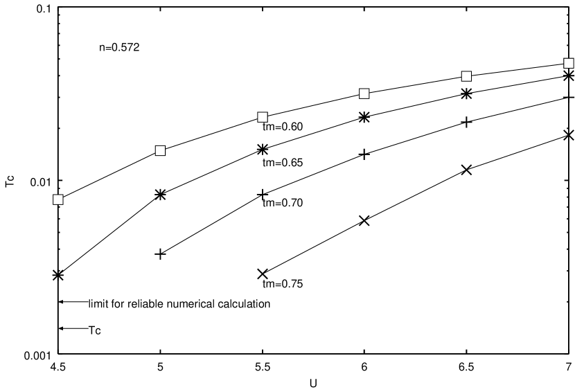
Figure 6: The calculated $T_{\rm c}$ as $U$ is varied, at $n=0.572$ and for various values of $t_{\rm m}$ as shown in the figure.

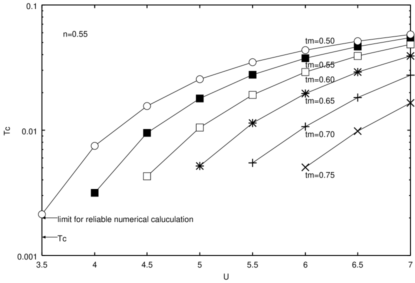
Figure 7: The calculated $T_{\rm c}$ as $U$ is varied, at $n=0.55$ and for various values of $t_{\rm m}$ as shown in the figure.

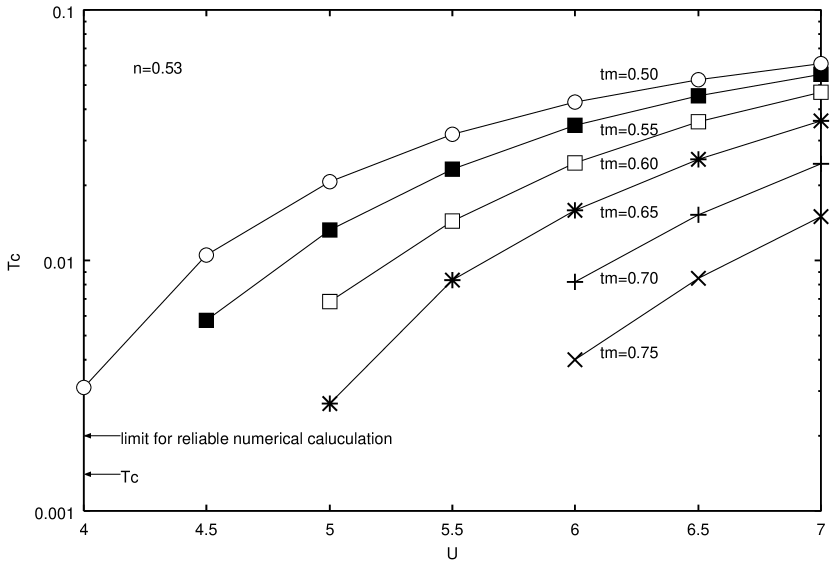
Figure 8: The calculated $T_{\rm c}$ as $U$ is varied, at $n=0.53$ and for various values of $t_{\rm m}$ as shown in the figure.

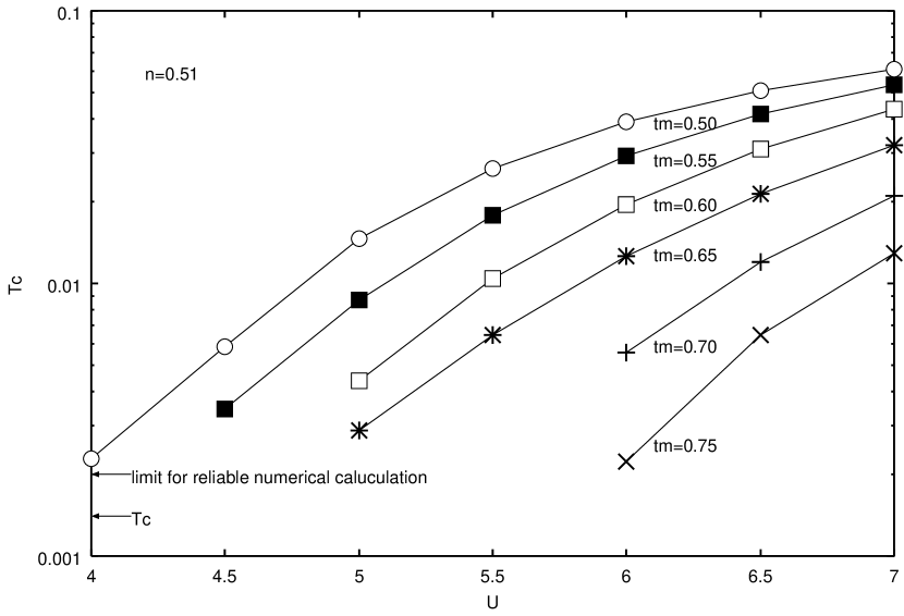
Figure 9: The calculated $T_{\rm c}$ as $U$ is varied, at $n=0.51$ and for various values of $t_{\rm m}$ as shown in the figure.

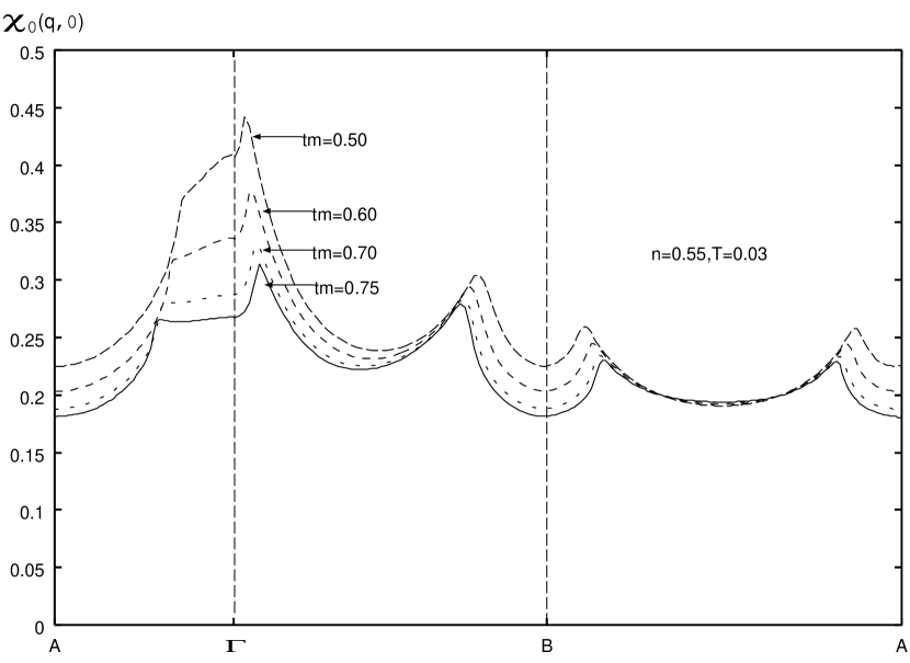
Figure 12: The momentum dependence of the static bare susceptibility for various $t_{\rm m}$. The notations under the horizontal axis are defined in Fig.2. These results are obtained for $n=0.55$, $T=0.03$.

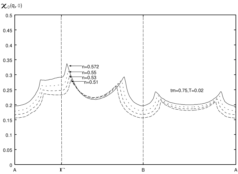
Figure 13: The momentum dependence of the static bare susceptibility for various $n$. The notations under the horizontal axis are defined in Fig.2. These results are obtained for $t_{\rm m}=0.75$, $T=0.02$.

References

- [1] C. Geibel, C. Schank, S. Thies, H. Kitazawa, C. D. Bredl, A. Bhm, M. Rau, A. Grauel, R. Caspary, R. Helfrich, U. Ahleim, G. Weber and F. Steglich: Z. Phys. B 84 (1991) 1.
- [2] A. Krimmel, P. Fischer, B. Roessli, H. Maletta, C. Geibel, C. Schank, A. Grauel, A. Loidl and F. Steglich: Z. Phys. B 86 (1992) 161.
-
[3]
R. Casparty, P. Hellmann, M. Keller, G. Sparn,
C. Wassilew,
R. Khler, C. Geibel, C. Shank, F. Steglich and N. E. Phillips: Phys. Rev. Lett. 71 (1993) 2146. -
[4]
R. Feyerherm, A. Amato, F. N. Gygax, A. Schenck,
C. Geibel, F. Steglich, N. Sato and T. Komatsubara: Phys. Rev. Lett. 73 (1994) 1849. - [5] M. Hiroi, M. Sera, N. Kobayashi, Y. Haga, E. Yamamoto and Y. : J. Phys. Soc. Jpn. 66 (1997) 1595.
- [6] L. M. Sandratskii, J. K, P. Zahn and I. Mertig: Phys. Rev. B 50 (1994) 15834.
- [7] K. Kn, A. Mavromaras, L. M. Sandratskii and J. K: J. Phys. 8 (1996) 901.
- [8] Y. Inada, H. Yamagami, Y. Haga, K. Sakurai, Y. Tokiwa, T. Honma, E. Yamamoto, Y. Onuki and T. Yanagisawa: J. Phys. Soc. Jpn. 68 (1999) 3643.
- [9] H. Yamagami (private comunications).
-
[10]
M. Kyogaku, Y. Kitaoka, K. Asayama, C. Geibel,
C. Schank and
F. Steglich: J. Phys. Soc. Jpn.62 (1993) 4016. - [11] K. Matsuda, Y. Kohori and T. Kohara: Phys. Rev. B 55 (1997) 15223.
- [12] K. Matsuda, Y. Kohori, T. Kohara: Physica B 259-261(1999) 640.
-
[13]
T. Petersen, T. E. Mason, G. Aeppli,
A. P. Ramirez,
E. Bucher, R. N. Kleiman: Physica B 199-200 (1994) 151. - [14] N. Metoki, Y. Haga, Y. Koike and Y. nuki: Phys. Rev. Lett. 80 (1997) 5417.
- [15] N. Metoki, Y. Haga, Y. Koike, N. Aso and Y. nuki: J. Phys. Soc. Jpn. 66 (1997) 2560.
-
[16]
N. Sato, N. Aso, G. H. Lander, B. Roessli,
T. Komatubara and
Y. Endoh: J. Phys. Soc. Jpn. 66 (1997) 1884. - [17] N. Bernhoeft, N. Sato, B. Roessli, N. Aso, A. Hiess, G. H. Lander, Y. Endoh and T. Komatubara: Phys. Rev. Lett. 81 (1998) 4244.
- [18] N. Bernhoeft, B. Roessli, N. Sato, N. Aso, A. Hiess, G. H. Lander, Y. Endoh, T. Komatubara: Physica B 259-261(1999) 614
- [19] M. Jourdan, M. Hunth, P. Haibach, H. Adrian: Physica B 259-261 (1999) 621.
- [20] M. Jourdan, M. Hunth and H. Adrian: Nature 398 (1999) 47.
- [21] T. Hotta: J. Phys. Soc. Jpn. 63 (1994) 4126.
- [22] T. Jujo, S. Koikegami and K. Yamada: J. Phys. Soc. Jpn. 68 (1999) 1331.
- [23] T. Nomura and K. Yamada: J. Phys. Soc. Jpn. 69 (2000) 3678.
- [24] M. Hunth, M. Jourdan and H. Adrian: Eur. Phys. J. B 13 (2000) 695.
- [25] K. Miyake and N. K. Sato: Phys. Rev. B 63 (2001) 52508.
-
[26]
N. K. Sato, N. Aso, K. Miyake, R. Shiina,
P. Thalmeier,
G. Varelogiannis, C. Geibel, F. Steglich, P. Fulde and
T. Komatsubara: Nature 410(2001)340. -
[27]
Y. Inada, Y. Haga, H. Okuni, Y. Tokiwa, R. Settai,
T. Honma,
E. Yamamoto and Y. nuki: Physica B 284-288 (2000) 523.