How backscattering off a point impurity can enhance the current and make the conductance greater than $e^{2}/h$ per channel

Abstract

It is well known that while forward scattering has no effect on the conductance of one-dimensional systems, backscattering off a static impurity suppresses the current. We study the effect of a time-dependent point impurity on the conductance of a one-channel quantum wire. At strong repulsive interaction (Luttinger liquid parameter $g<1/2$), backscattering renders the linear conductance greater than its value $e^{2}/h$ in the absence of the impurity. A possible experimental realization of our model is a constricted quantum wire or a constricted Hall bar at fractional filling factors $\nu=1/(2n+1)$ with a time-dependent voltage at the constriction.

I Introduction

There are several motivations to study one-dimensional (1D) quantum conductors. Quantum wires are expected to be an essential component of future nanoelectronic devices. The analogy between 1D electron liquid and edge states of the 2D electron gas is conducive to the understanding of the Quantum Hall effect [1]. There are also many other related systems such as vortex lines in type-II superconductors [2]. From the theoretical point of view 1D conductors are the simplest non-Fermi-liquid systems. Probably, the most appealing consequence of non-Fermi-liquid behavior is the existence of fractionally charged quasiparticles, recently observed in experiments on Quantum Hall systems [3]. Since the experimental setup was based on a realization of 1D quantum wire with an impurity, the latter problem has received considerable renewed attention.

The effect of an impurity on a gas of noninteracting electrons is evident. It leads to backscattering, hence to suppression of the current. Qualitatively the same happens in the case of a static impurity in the presence of electron-electron interaction too. However, in that case the effect turns out to be counterintuitively strong. Even an arbitrarily weak impurity renders the conductance of a long wire equal to zero, thus effectively cutting the wire into two independent pieces [4, 5, 6]. This is yet another manifestation of strong correlations in a non-Fermi-liquid state.

While recent activity has focused primarily on the problem of static impurities, it is also interesting to understand what happens if the impurity potential depends on time. This question touches upon the problem of pumping [7] and the effect of phonon pulses in 1D conductors [8]. Recent works [9] consider the effect of a time-dependent impurity on Fermi-liquid states. Much less attention was devoted to the interplay between a time-dependent impurity and non-Fermi-liquid effects [10]. In this article we study the simplest question of this type: how a weak, point-like impurity whose potential depends on time affects the conductance of a quantum wire with a repulsive electron-electron interaction. In the absence of interaction the answer would be obvious. The impurity would decrease the current, the suppression of the current depending on the strength of the impurity potential. Surprisingly, for interacting systems the time-dependent backscattering impurity can enhance the conductance. This is the main result of the present Letter. Such enhancement takes place as the interaction strength exceeds a threshold value. In terms of the Luttinger liquid parameter $g$ the threshold is $g=1/2$. We would like to emphasize that the predicted current enhancement is a linear effect, and the linear conductance of a one-channel wire becomes greater than the conductance quantum $e^{2}/h$ for strong repulsive interactions.

The paper is organized as follows: first we discuss the origin of the effect qualitatively. In the third section we formulate our model and discuss the details of the set-up (e.g. the way how the voltage is applied). In the forth section details of calculations are discussed. In conclusion we discuss the results and possible experimental realizations.

II Qualitative discussion

Let us first discuss the origin of the effect qualitatively. While a purely qualitative discussion is insufficient to explain the threshold value $g=1/2$, we show below that our effect can be derived heuristically from a simple analysis of the structure of the Hamiltonian. Our detailed analysis yields quantitative results concerning the weak impurity limit and is based on the bosonization technique [11].

Using the analogy between a quantum wire and edge states of the 2D electron gas [12], we interpret backscattering off a weak impurity as tunneling between two chiral systems of right- and left-movers. The tunneling density of states diverges as the energy approaches the Fermi energy [13]. In other words, backscattering is enhanced in the two following cases: 1) the energy of the incident particle is close to the Fermi energy of the electrons moving in the same direction; 2) the energy of the backscattered particle is close to the Fermi energy of the electrons which move in the direction opposite to that of the incident particle. The left and right Fermi energies differ by the applied voltage $V$. These statements about the dependence of the backscattering amplitude on the energy do not hold for noninteracting electrons. In that case one should only note that scattering to an occupied state is impossible. The energy dependence is more pronounced for the stronger electron-electron interaction.

Now we are in a position to consider a time-dependent impurity. Let us assume for simplicity that the time-dependent potential is harmonic, $W(t)\sim U\cos\omega t$. Note, however, that the current enhancement is possible for a general periodic potential. In our qualitative discussion we consider the case $\hbar\omega>eV;\hbar\omega\approx eV$, where $V$ is the voltage and $e=-|e|$ – the electron charge. In this case we predict particularly strong current enhancement. We assume that the Fermi energy of the particles moving to the left is $E_{\rm FL}=eV$ and the Fermi energy of the right-movers – $E_{\rm FR}=0$. The scattering is inelastic. For small $U$ only processes involving an emission (absorption) of a single quantum are allowed, hence the energy change is $\pm\hbar\omega$. There are four backscattering processes (Fig. 1) which we denote as $L^{\pm},R^{\pm}$, where the letter shows the type of particles (left- or right-movers) and the $+/-$ sign corresponds to increasing/decreasing the energy of the particle. The processes $R^{-}$ and $L^{-}$ are suppressed by the Pauli principle since they lead to the scattering into states which are below the Fermi energies, $E_{\rm FL}$ and $E_{\rm FR}$ respectively. The processes $L^{+}$ and $R^{+}$ drive particles into states above the Fermi energy. However, only $R^{+}$ processes lead to the scattering of the particles with initial energy around $E_{\rm FR}$ to final states with energy close to $E_{\rm FL}$. As discussed above, for such particles the probability of backscattering is enhanced. For $L^{+}$ processes the particles with the initial energy close to $E_{\rm FL}$ are backscattered into the states whose energies are not close to $E_{\rm FR}$. Hence, the backscattering amplitude for such processes is less than for $R^{+}$ processes. On the other hand, $L(R)^{+}$ processes are effective for particles with energies $E$ in the interval $E_{\rm FL(FR)}>E>E_{\rm FR(FL)}-\hbar\omega$, where $E_{\rm FL}>E_{\rm FR}$ (cf. Fig. 1). Hence the number of left-moving particles which potentially can be subject to strong $L^{+}$ backscattering processes exceeds the number of right-movers which potentially are subject to $R^{+}$ processes [14]. As the electron-electron interaction increases, $R^{+}$ becomes more important. At some threshold the latter begins to provide the main contribution to the backscattering current, hence it determines its direction. Since this process modifies right-movers to left-movers, such backscattering enhances the current. Thus, paradoxically, the scattering of particles backwards adds electrons to the forward flow.

The above qualitative discussion was based on an effective single-particle picture. Certainly, our systematic approach that leads to essentially the same conclusions does not rely on such a simplified picture.

Two important ingredients of the above arguments are inelastic backscattering and energy dependence of the backscattering amplitude. Both conditions can be realized in a non-interacting system. This will not however result in current enhancement since the third key ingredient is missing: Backscattering amplitudes in a non-interacting system depend only on the absolute value of the electron momentum but not on its direction in the case of symmetric geometry considered in this paper. On the other hand, in the absence of the symmetry in a non-interacting system, one gets generation of the photocurrent instead of enhancement of the injected current. The direction of the photocurrent is not related to the sign of the voltage and it can flow at zero voltage.

III Model and sketch of derivation

Below we provide a quantitative theory (valid for general $V,\omega$).

We consider spinless electrons [15] and concentrate first on the case of zero temperature. Our starting point is the Tomonaga-Luttinger model [5, 11] with a point impurity. The Hamiltonian reads

$$H=\int dx[-\hbar v_{F}(\psi_{R}^{\dagger}(x)i\partial_{x}\psi_{R}(x)-\psi_{L}^{\dagger}(x)i\partial_{x}\psi_{L}(x))+K(x)(\psi^{\dagger}_{R}(x)\psi_{R}(x)+\psi^{\dagger}_{L}(x)\psi_{L}(x))^{2}$$ (1)

$$+\delta(x)W(t)(\psi^{\dagger}_{L}(0)\psi_{R}(0)+\psi^{\dagger}_{R}(0)\psi_{L}(0))],$$ (2)

where $\psi_{R}$ and $\psi_{L}$ are the fermionic field operators of the right- and left-moving electrons, $v_{F}$ is the Fermi velocity, $W(t)$ the potential of the impurity located at the origin and $K(x)$ – the interaction strength. We take $K(x)=K$ in the region $-L/2<x<L/2$, and $K=0$ at $|x|\gg L$. Thus, we assume that the electron-electron interaction is completely screened at large $x$. Below we set $v_{F}$ and $\hbar$ equal to unity. We assume that the right- and left-movers are injected from the leads with chemical potentials $\mu_{R}=0;\mu_{L}=eV>0$. Note that in our notation $\mu_{L}$ is located on the right (Fig. 1).

We use a set-up in which the interaction strength $K=0$ in the right and left parts of the system. This is the model used in Ref. [17]. There are many approaches to model leads, the bias voltage, and other details of the systems. They reflect different possible set-ups. Some details of the behavior may be sensitive to the details of the set-up. We limit our discussion by the set-up used in Ref. [17].

The choice of the Hamiltonian in the form (1) assumes that the interaction is short range. This means that the Coulomb interaction between electrons is screened (by the gates) [18].

We follow the technical procedure developed in Ref. [16] for a static impurity. We employ the Keldysh formalism [19]. At $t=-\infty$ the impurity potential is absent, $W(t)=0$, and then it is gradually turned on. Thus, at the initial moment of time the Hamiltonian (1) is time-independent and commutes with the operators of the numbers of right- and left-moving particles $\hat{N}_{R}$ and $\hat{N}_{L}$. Hence, initially the system can be described by the partition function with two chemical potentials $\mu_{R}=0$ and $\mu_{L}=eV$ conjugated with the particle numbers $N_{R}$ and $N_{L}$.

It is convenient to switch to the interaction representation $H\rightarrow H-\mu_{R}N_{R}-\mu_{L}N_{L}$. This transformation introduces time dependence into the $\psi_{L}$ operator. Thus, we have to substitute $\psi_{L}\rightarrow\psi_{L}\exp(-ieVt)$, $\psi_{L}^{\dagger}\rightarrow\psi_{L}^{\dagger}\exp(ieVt)$ in every expression where those operators enter. In particular, the impurity contribution in Hamiltonian (1) now reads $\delta(x)W(t)(\psi^{\dagger}_{L}(0)\psi_{R}(0)\exp(i\omega_{0}t)+h.c.)$, where $\omega_{0}\equiv eV$.

Next, we derive an expression for the current operator. The current includes the background contribution from the particles injected from the leads and the backscattering contribution associated with the impurity and proportional to the backscattering rate. The background contribution is equal to the current in the absence of the impurity. Since $\mu_{L}>0$, the background particle current (of particles with $e<0$) flows to the left.

The background current is simply $I_{0}=e^{2}V/h$ [17]. The backscattering contribution is time-dependent due to the non-stationary nature of our problem. The dc contribution to the total current must be independent of the coordinates due to the charge conservation. Hence, it can be represented in two equivalent forms:

$$I_{dc}=I_{L}^{\leftarrow}-I_{L}^{\rightarrow}=I_{R}^{\leftarrow}-I_{R}^{\rightarrow},$$ (3)

where $I_{L}^{\rightarrow}$ and $I_{R}^{\leftarrow}$ are the currents of right- and left-movers injected form the left and right leads respectively, $I_{L}^{\leftarrow}$ and $I_{R}^{\rightarrow}$ are the currents of left- and right-movers incident to the left and right leads respectively. The difference $I_{L}^{\leftarrow}-I_{R}^{\leftarrow}=\overline{dN_{L}/dt}$, where the bar denotes the time average, $dN_{L}/dt$ is the change in the number of left-movers in the wire due to backscattering off the impurity. Hence, $I_{dc}=I_{R}^{\leftarrow}-I_{L}^{\rightarrow}+\overline{dN_{L}/dt}$. The currents of injected particles $I_{R}^{\leftarrow}$ and $I_{L}^{\rightarrow}$ are the same in the absence and in the presence of the impurity. Finally, we obtain for the dc current

$$I_{dc}=\frac{e^{2}V}{h}+e\overline{\frac{dN_{L}}{dt}}.$$ (4)

Thus, the backscattering particle current can be defined as $\hat{I}_{\rm bs}=d\hat{N}_{L}/dt=-d\hat{N}_{R}/dt$, where $\hat{N}_{L}$ and $\hat{N}_{R}$ are the particle number operators. A positive value of the backscattering current corresponds to the enhancement of the background current. In terms of the $\psi$-fields the backscattering current operator (in the interaction representation) is given by the equation

$$\hat{I}_{\rm bs}=-iW(t)(\psi^{\dagger}_{L}(0)\psi_{R}(0)\exp(i\omega_{0}t)-h.c.).$$ (5)

Since $W(t)\sim\cos\omega t$, one finds that there are two types of time-dependent terms in the Hamiltonian and the current operator: (i) terms proportional to $\exp(\pm i(\omega+\omega_{0})t)$ and (ii) terms proportional to $\exp(\pm i(\omega-\omega_{0})t)$. If only terms of the first (second) type existed our problem would be equivalent to a static impurity in the presence of an external voltage drop $V_{1(2)}=(\omega_{0}\pm\omega)/e$ (in the appropriate interaction representation). Hence, the backscattering current can be represented as $I_{\rm bs}=I_{1}+I_{2}+I_{12}$, where $I_{1,2}$ denotes the backscattering current in the static problem with the voltage $V_{1,2}$, and $I_{12}$ is the ’interference’ contribution. We will see that to the lowest order in the impurity potential the interference current $I_{12}$ is ac, hence the dc-current is made of $I_{1}$ and $I_{2}$ only. Hence if one is interested in the averages over time $t>1/\omega$, the contribution $I_{12}$ drops out. We know from Ref. [5] that $I_{1,2}\sim|V_{1,2}|^{2g-1}$, where $g=\sqrt{\pi\hbar v_{F}/(\pi\hbar v_{F}+2K)}$ is the standard dimensionless parameter of the Luttinger liquid. For $g<1/2$ the exponent $2g-1$ is negative, hence the main contribution to $I_{\rm bs}$ is $I_{2}$. Thus the direction of the backscattering current is the same as in the static problem with the voltage $V_{2}$. At $\omega>\omega_{0}$ the sign of this voltage is opposite to the sign of the applied voltage $V$. This shows that the backscattering current enhances the background one.

IV Quantitative analysis

In order to actually calculate the currents $I_{\rm dc}=I_{1}+I_{2}$ and $I_{\rm ac}=I_{12}$ we employ the bosonization transformation [11, 16]. This leads to the action

$$L=\int dtdx\biggl{[}\frac{1}{8\pi}((\partial_{t}\hat{\Phi})^{2}-(\partial_{x}\hat{\Phi})^{2})-\delta(x)W(t)(e^{i\sqrt{g}\hat{\Phi}(t,x=0)}e^{i\omega_{0}t}+h.c.)\biggr{]},$$ (6)

where $W(t)=U\cos\omega t$ and the bosonic field $\hat{\Phi}$ is related to the charge density as $\hat{\rho}=e\sqrt{g}\partial_{x}\hat{\Phi}/(2\pi)$. The same action describes a quantum Hall bar with a (time-dependent) constriction [12]. In that case $g$ is the filling factor $g=1/(2n+1)$. The current operator reads

$$\hat{I}_{\rm bs}=-iW(t)e^{i\sqrt{g}\hat{\Phi}(t,x=0)}e^{i\omega_{0}t}+h.c.$$ (7)

To find the backscattering current at the moment $t$ we have to calculate the average

$$\langle\hat{I}_{\rm bs}(t)\rangle=\langle 0|S(-\infty;t)\hat{I}_{\rm bs}(t)S(t;-\infty)|0\rangle,$$ (8)

where $\langle 0|$ denotes the initial state, $S$ is the scattering matrix. As we remember from the previous section, the initial state is defined in terms of the two chemical potentials of the right- and left-movers. To the lowest order in $W$

$$S(t;-\infty)=1-i\int_{-\infty}^{t}dt^{\prime}[W(t^{\prime})e^{i\sqrt{g}\hat{\Phi}(t^{\prime},x=0)}e^{i\omega_{0}t^{\prime}}+h.c.];S(-\infty;t)=S^{*}(t;-\infty).$$ (9)

Further calculations follow the standard route [16] and show that the current $I=I_{\rm dc}+I_{\rm ac}$ includes a dc-contribution $I_{\rm dc}$ and an ac-contribution $I_{\rm ac}$ of frequency $2\omega$. One evaluates expression (8) using the Green function of the Bose field:

$$\langle 0|\Phi(t)\Phi(0)|0\rangle=-2\ln(\delta+it),$$ (10)

where $\delta$ is infinitesimal. We first discuss the more interesting dc-contribution. It has different forms at $\omega>\omega_{0}=eV$ and $\omega<\omega_{0}$ (cf. Fig. 2)

$$I_{\rm dc}=\frac{U^{2}}{2(v_{F}\tau_{c})^{2}}\Gamma(1-2g)\tau_{c}^{2g}\sin(2\pi g)[(\omega-\omega_{0})^{2g-1}-(\omega+\omega_{0})^{2g-1}],~{}~{}~{}\omega>\omega_{0};$$ (11)

$$I_{\rm dc}=-\frac{U^{2}}{2(v_{F}\tau_{c})^{2}}\Gamma(1-2g)\tau_{c}^{2g}\sin(2\pi g)[(\omega_{0}-\omega)^{2g-1}+(\omega+\omega_{0})^{2g-1}],~{}~{}~{}\omega<\omega_{0},$$ (12)

where $\tau_{c}\sim 1/E_{\rm Fermi}$ is a short-time cutoff. While at $g>1/2$ the current $I_{\rm dc}<0$ in both cases, at strong interaction, $g<1/2$, the backscattering current becomes positive as $\omega>\omega_{0}$. In other words, in the latter case it flows in the direction of the background current. In the limit $\omega_{0}\rightarrow 0$ one finds a correction to the conductance (which would be equal to $G=e^{2}/h$ in the absence of the impurity [17]). The correction

$$\Delta G=\frac{e^{2}}{\hbar^{3}}\left(\frac{U}{v_{F}\tau_{c}}\right)^{2}(1-2g)\omega^{2g-2}\Gamma(1-2g)\tau_{c}^{2g}\sin(2\pi g)$$ (13)

is positive for $g<1/2$. The generalization to the case when the time-dependent potential $W(t)$ contains several harmonics is straightforward.

The results (11,12) are obtained at zero temperature. As $T>|\omega-\omega_{0}|$ the expression for the current is modified. The effect of finite temperature can be determined with the Keldysh technique [19]. To avoid cumbersome expressions we discuss here only the limiting cases. A full expression for the current has the opposite sign and the same absolute value as the sum of two expressions of the form (A5) [5] with $a(t)=(\omega_{0}\pm\omega)t$ and $g\rightarrow 1/g$. At low temperatures $\omega+\omega_{0}>T>|\omega-\omega_{0}|$ the backscattering current is given as the sum of two terms, proportional to $(\omega-\omega_{0})T^{2g-2}$ and to $(\omega+\omega_{0})^{2g-1}$ respectively. The current becomes positive (enhancement of the total current) for $\omega>\omega_{0}$, $T<(\omega+\omega_{0})\left(\frac{\omega-\omega_{0}}{\omega+\omega_{0}}\right)^{1/(2-2g)}$. As $T\gg\omega,V$ the dependence of the backscattering current on $\omega$ drops out. The latter turns out to be always negative: $I_{\rm bs}\sim-\omega_{0}T^{2g-2}$.

There is also an ac contribution of frequency $2\omega$ to the current. At $T=0$ it reads as follows

$$I_{\rm ac}(t)=\left(\frac{U}{v_{F}\tau_{c}}\right)^{2}\Gamma(1-2g)\tau_{c}^{2g}\cos(\pi g+2\omega t)\sin(\pi g)[(\omega-\omega_{0})^{2g-1}-(\omega+\omega_{0})^{2g-1}],\omega>\omega_{0};$$ (14)

$$I_{\rm ac}(t)=-\left(\frac{U}{v_{F}\tau_{c}}\right)^{2}\Gamma(1-2g)\tau_{c}^{2g}\sin(\pi g)[\cos(2\omega t-\pi g)(\omega_{0}-\omega)^{2g-1}+\cos(2\omega t+\pi g)(\omega+\omega_{0})^{2g-1}],\omega<\omega_{0}.$$ (15)

In our model we neglect forward scattering at the impurity. This approximation is valid in the case of a weak impurity. Indeed, both forward and backscattering terms in the Hamiltonian have order $U$. The backscattering current includes three contributions: one goes solely from backscattering, the second solely form the forward scattering term, the third is the interference contribution. The second contribution is zero: forward scattering alone cannot modify the current. The interference contribution is zero up to the second order in $U$. Indeed, the backscattering current operator $d\hat{N}_{L}/dt=i[\hat{H},\hat{N}_{L}]/\hbar$ has the same form (5) both in the presence and in the absence of forward scattering. Hence, the interference contribution can be found from Eq. (8). For this one has to add a forward scattering term to the expansion of the $S$-matrix up to the first power of $U$ Eq. (9). A simple calculation shows that the resulting interference correction is zero indeed up to the order $U^{2}$. Nonzero corrections are possible in higher orders.

Thus, our calculations are restricted by the case of a weak impurity. Note that the current enhancement is impossible for a strong impurity: An infinite barrier cuts the systems into two independent pieces and the total current is just zero. Hence, there is a critical impurity strength at which our effect disappears.

V Conclusion

A possible experimental realization of our system is a one dimensional wire in the presence of a time-dependent gate voltage that allows to obtain a time-dependent constriction in one point. External magnetic field must polarize electrons in the wire.

Another possible experimental realization of our model is a Hall bar with a constriction [20]. The role of the backscattering impurity is played by the constriction that gives rise to weak tunneling of quasiparticles between the two edges. The tunneling amplitude can then be made time-dependent by application of a time-dependent gate voltage. If the system is tuned such that it is close to a resonance [5] then it can be described by the Lagrangian (6) with $W(t)=U\cos\omega t$. In the absence of tuning a static contribution $W_{0}$ should be added to $W(t)$. Still if the inter-edge tunneling is weak and $\omega$ is greater than the product of the voltage difference between the edges and the quasiparticle charge, we expect an enhancement of the Hall current in the FQHE (at filling factors $g=1/(2n+1)$) as compared with the absence of a time-dependent perturbation both at $W_{0}>W$ and $W_{0}<W$. On the other hand, the time-dependent tunneling decreases the current in IQHE where the filling factor $g=1$.

Both in IQHE and FQHE cases our system can be interpreted as a rectifier: It transforms an ac gate voltage into a dc current. There is also a relation between our problem and pumping [7]. Pumping requires two time-dependent parameters while in our problem there is only one such parameter, the impurity strength. However, as we have discussed, for the calculation of the backscattering current the voltage can be gauged out giving rise to an additional time-dependent parameter. Thus, the backscattering current can be interpreted as a pumped current. There is also an analogy between our problem and photon assisted current: in both cases there is a time-dependent parameter and the left-right symmetry is broken (in our case by the voltage).

A more general question concerns the effect of external noise on the quantum wire. One can consider the tunneling amplitude $W(t)=\int d\omega[{U^{\prime}}_{\omega}\cos\omega t+{U^{\prime\prime}}_{\omega}\sin\omega t]$, where $\langle({U^{\prime}}_{\omega})^{2}\rangle=\langle({U^{\prime\prime}}_{\omega})^{2}\rangle=S(\omega)$ is the spectral function of the noise. The simplest realization of a random $W(t)$ are thermal fluctuations of the gate voltage in the set-up discussed in the previous paragraphs. Another related problem is the effect of the irradiation by phonons. If a hot spot is created in the region of the constriction then phonons give rise to a time-dependent backscattering. The total backscattering current can be obtained from Eqs. (11,12) integrating over $\omega$ and substituting $2S(\omega)$ for $U^{2}$. Note that for white noise, $S(\omega)={\rm const}$, the backscattering current calculated in such way vanishes at $g<1/2$. Note however, that a mathematically ideal white noise includes frequencies which are higher than the Fermi energy. At such frequencies an approach based on the Luttinger model cannot be used. This will result in small non-zero corrections to the conductance.

In conclusion, we have found that backscattering off a point impurity can increase the conductance of a quantum wire. This is a manifestation of the strong electron-electron interaction as the Luttinger liquid parameter $g<1/2$.

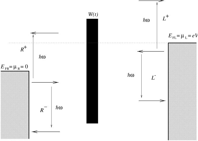
FIG. 1.: Right-moving electrons with Fermi energy $E_{\rm FR}=\mu_{\rm R}=0$ and left-moving electrons with Fermi energy $E_{\rm FL}=\mu_{\rm L}=eV$ are backscattered off the time-dependent impurity $W(t)$ via $R^{\pm}$ and $L^{\pm}$ processes in which the electrons gain or lose an energy quantum $\hbar\omega$.

FIG. 2.: Qualitative dependence of the backscattering contribution $I_{\rm dc}$ to the dc-current on the frequency $\omega$ at $g<1/2$. $\omega_{0}=eV/\hbar$, where $V$ is the applied voltage. Note that $I_{\rm dc}>0$ as $\omega>\omega_{0}$ (total current enhanced). Our approach based on the lowest order of the perturbation theory is insufficient for the region $\omega\approx\omega_{0}$.

- [1] Perspectives in Quantum Hall Effects, edited by S. Das Sarma and A. Pinczuk (John Wiley & Sons, Inc., New York, 1997).
- [2] A. Vishwanath and T. Senthil, Phys. Rev. B 63, 014506 (2001).
- [3] R. de Piccioto, M. Reznikov, M. Heiblum, V. Umansky, G. Bunin, and D. Mahalu, Nature 389, 6647 (1997); L. Saminadayar, D.C. Glattli, Y. Jin, and B. Etienne, Phys. Rev. Lett. 79, 2526 (1997).
- [4] D.C. Mattis and E.H. Lieb, J. Math. Phys. 6, 304 (1965).
- [5] C. L. Kane and M. P. A. Fisher, Phys. Rev. B 46, 15233 (1992).
- [6] Y. Oreg and A.M. Finkelstein, Phys. Rev. Lett. 76, 4230 (1996).
- [7] B.L. Altshuler and L.I. Glazman, Science 283, 1864 (1999).
- [8] A. J. Kent, D. J. McKitterick, L. J. Challis, P. Hawker, C. J. Mellor, and M. Henini, Phys. Rev. Lett. 69, 1684 (1992); V. I. Talyanskii, J. M. Shilton. M. Pepper. C. G. Smith, C. J. B. Ford, E. H. Linfeld, D. A. Ritchie, and G. A. C. Jones, Phys. Rev. B 56, 15180 (1997).
- [9] See, e.g., S. Datta and M.P. Anantram, Phys. Rev. B 45, 13761 (1992); Y. Levinson and P. Wolfle, Phys. Rev. Lett. 83, 1399 (1999).
- [10] P. Sharma and C. Chamon, Phys. Rev. Lett. 87, 096401 (2001); D. Schmeltzer, Phys. Rev. B 63, 125332 (2001).
- [11] For reviews see, e.g., S. Rao and D. Sen, e-print cond-mat/0005492; J. von Delft and H. Schoeler, Annalen Phys. 7, 225 (1998).
- [12] X.-G. Wen, Int. J. Mod. Phys. B 6, 1711 (1992).
- [13] J.M. Kinaret, Y. Meir, N.S. Wingreen, P.A. Lee, and X.-G. Wen, Phys. Rev. B 46, 4681 (1992).
- [14] Note that when considering the product of the number of particles subject to backscattering and the probability for such a process, it is not a priori clear whether it is the or that win.
- [15] As possible realization one may consider a polarized electron liquid or an edge state of a quantum Hall bar. For electrons with spin the effective Luttinger parameter exceeds and our effect does not show up.
- [16] C. de C. Chamon, D. E. Freed, and X. G. Wen, Phys. Rev. B 51, 2363 (1995); throughout the paper we follow the notation of this reference.
- [17] D.L. Maslov and M. Stone, Phys. Rev. B 52, 5539 (1995); V.V. Ponomarenko, Phys. Rev. B 52, 8666 (1995); I. Safi nad H.J. Schulz, Phys. Rev. B 52, 17040 (1995).
- [18] The electric potential in the point is proportional to the energy cost of adding an infinitesimal charge to this point. From the Hamiltonian (1) one finds that , where is the interaction strength, the charge density. One sees that at i.e. in the regions where the electron-electron interaction is completely screened in the left and right parts of the wire. Thus, the voltage drop between these two region is always zero. This does not contradict the fact that one can apply a finite voltage between the leads: the voltage drop occurs in the contacts between the leads and the wire. Note also that the electric potential is nonzero in the region in the center of the wire. It depends on in a non-monotonous way since at .
- [19] J. Rammer and H. Smith, Rev. Mod. Phys. 58, 323 (1986); A. Kamenev, e-print cond-mat/0109316.
- [20] F. P. Milliken, C. P. Umbach, and R. A. Webb, Solid State Commun. 97, 309 (1996).