[

Non-Perturbative Aspects of Fano Resonances in Quantum Dots: An Exact Treatment

Abstract

We consider transport through quantum dots with two tunneling paths. Interference between paths gives rise to Fano resonances exhibiting Kondo-like physics. In studying such quantum dots, we employ a generalized Anderson model which we argue to be integrable. The exact solution is non-perturbative in the tunneling strengths of both paths. By exploiting this integrability, we compute the zero temperature linear response conductance of the dot and so obtain reasonable quantitative agreement with the experimental measurements reported in Göres et al. PRB 62, 2188 (2000).

]

In recent years advances in nanotechnology have made possible the fabrication of single electron transistors (SETs). SETs, or colloquially, quantum dots, are characterized by the remarkable ability to tune, via a gate voltage, the number of localized electrons sitting upon the dot. By tuning the number of electrons to be nearly one, a novel Kondo system is created. This new realization of an old physical paradigm has sparked tremendous experimental interest, i.e. [3, 4].

In the simplest realization of quantum dots there exists a single conduction path through the dot. However the flexibility inherent in semi-conductor SETs allows for more exotic scenarios. Dots may be fabricated such that multiple tunneling paths are activated. Generically the presence of multiple tunneling paths leads to interference effects observable in transport properties. In the presence of two tunneling paths, one resonant (i.e. energy dependent), one not, Fano resonances can arise [5]. Such resonances in quantum dots have been observed [1, 2] in the form of asymmetric peaks and dips in the linear response conductance as a function of the gate voltage.

Although this letter will focus upon the observations of [1], Fano resonances are ubiquitous in nanodevices. Quantum dots have been embedded in multiple connected geometries permitting precise delineation of possible tunneling paths. Such geometries, in addition, allow threading by Aharonov-Bohm fluxes. The behaviour of transport in such devices has been studied in [8]. Fano resonances have also been observed in STM measurements of adsorbed magnetic atoms on metallic substrates. Here interference occurs because of an interplay between the Kondo resonance and tunneling into the continuum of surface conduction electrons [7, 6].

The appearance of Fano resonances in quantum dots occurs in conjunction with Kondo-like phenomena. Fano resonances reported in [1] shows a logarithmic dependence upon temperature reminiscent of the Kondo effect. In addition the authors of [1] observe a sharp dependence of the Fano resonances upon small magnetic fields. Although attributed to a loss of coherent transport in the resonant scattering channel, it might also represent the destruction of a putative Kondo effect in the dots. Observations of Fano resonances in STM tunneling experiments [6] are directly related to a Kondo resonance arising from the proximity of a magnetic adatom.

To model Fano resonances we generalize the standard two lead Anderson model in the simplest possible way by adding a direct lead-lead coupling. In the standard model electrons transit from one lead to the other through hopping on and off the dot. The direct lead-lead tunneling provides a competing scattering path, nominally independent of energy. The model Hamiltonian takes the form

$${\cal H} = H_{\rm Anderson}+H_{\rm lead-lead~{}tunneling}$$ (1)

$$= -i\sum_{l=L,R;~{}\sigma=\uparrow,\downarrow}\int^{\infty}_{-\infty}dxc_{l\sigma}^{\dagger}(x)\partial_{x}c_{l\sigma}(x)$$ (4)

$$+V_{dl}(c_{l\sigma}^{\dagger}(0)d_{\sigma}+{\rm h.c.})+\epsilon_{d}\sum_{\sigma}n_{\sigma}+Un_{\uparrow}n_{\downarrow}$$

$$+V_{LR}(c^{\dagger}_{L\sigma}(0)c_{R\sigma}(0)+{\rm h.c.}).$$

Here ${\cal H}$ encodes the standard Anderson model together with an additional term allowing electrons to transit directly from one lead to the other. The $c_{l\sigma}$’s/$d_{\sigma}$’s specify the lead/dot electrons with $n_{\sigma}=d^{\dagger}_{\sigma}d_{\sigma}$. $U$ measures the Coulomb repulsion on the dot while $\epsilon_{d}$ gives the dot single particle energy. $V_{ld}$ are the dot-lead hopping matrix elements. Experimental realizations of quantum dots generically see $V_{Ld}\neq V_{Rd}$. $V_{LR}$ marks the strength of the direct transmission channel. The spatial variable $x$ runs from $-\infty$ to $\infty$ reflecting the ‘unfolding’ of the leads [14].

In employing this model to describe the transport properties of dots such as those studied in [1], we assume that only a single level on the dot is relevant to transport. This requires the level broadening, $\Gamma\sim V^{2}$, to be considerably less than $U+\Delta\epsilon$, where $\Delta\epsilon$ is the level spacing. At least for a subset of the data in [1], this condition is met with $\Gamma/(U+\Delta\epsilon)\sim.1$. We note that in experimental measurements on dots with a single tunneling path[3], $\Gamma/(U+\Delta\epsilon)\sim 1/6$, yet the Anderson model does an excellent job of describing the scaling behaviour of the reported finite temperature linear response conductance.

The model also presumes that the second tunneling path is simply due to lead-lead hopping. While it is not entirely clear the quantum dots of [1] are so described, we will show this model more than adequately describes the observed phenomena. For dots embedded in a multiply connected geometry, i.e. [8], the ambiguity is lifted and this term provides a precise description of the second tunneling path. Fano resonances in quantum dots were described using random matrix theory in [9] where the exact nature of the direct path need not be specified. Aspects of the observations in Ref. [1] were described by this treatment. However Coulomb interactions were unable to be dealt with directly. As we will discuss we believe an exact treatment of the non-perturbative physics present at finite $U$ is necessary to describe the observations.

The two lead Anderson model with lead-lead tunneling has been studied previously [10, 11]. There the model was analyzed by expressing all the relevant correlators in terms of the dot Greens function $\langle d^{\dagger}d\rangle$ via a system of Dyson equations. The dot correlators are then computed via an equations of motion technique [10], or a numerical renormalization group [11]. In our exact treatment of the model we find qualitative differences with this approach. We believe this is a result of the non-perturbative physics inherent in the problem. Although the Dyson equations sum up all diagrams, they assume nonetheless the problem to be perturbative in the lead-lead coupling, $V_{LR}$. Our Bethe ansatz solution indicates this to not be the case. In particular for $U>0$, we do not find a smooth $V_{LR}\rightarrow 0$ limit. Perhaps this is not so unsurprising: we similarly have no expectation that the problem is perturbative in the dot-lead coupling, $V_{dl}$.

Analysis of model: We first examine the particular case of $V_{dR}=V_{dL}$. We will later show how this can be generalized. To argue that the model is thus integrable we recast the two lead Anderson model into an even/odd basis via the transformation,

$$c_{e/o}=(c_{L}\pm c_{R})/\sqrt{2}.$$

With this transformation the Hamiltonian becomes,

$${\cal H} = H_{e}+H_{o}$$ (5)

$${\cal H}_{e} = -i\sum_{\sigma}\int^{\infty}_{-\infty}dxc^{\dagger}_{e\sigma}(x)\partial_{x}c_{e\sigma}(x)+\epsilon_{d}\sum_{\sigma}n_{\sigma}$$ (7)

$$\hskip-10.84006pt+Un_{\uparrow}n_{\downarrow}+\Gamma^{1/2}(c^{\dagger}_{e}(0)d_{\sigma}+{\rm h.c.})+V_{LR}c^{\dagger}_{e\sigma}c_{e\sigma}|_{x=0};$$

$${\cal H}_{o} = -i\sum_{\sigma}\int^{\infty}_{-\infty}dxc^{\dagger}_{o\sigma}(x)\partial_{x}c_{o\sigma}(x)-V_{LR}c^{\dagger}_{o\sigma}c_{o\sigma}|_{x=0},$$ (8)

with $\Gamma=(V_{dL}^{2}+V_{dR}^{2})^{1/2}$ the total dot-lead coupling. Note that the dot only couples to the even electrons.

In changing to an even/odd basis we are still able to compute scattering amplitudes of electronic excitations off the dot. The even-odd excitations we employ scatter off the dot with a pure phase, $\delta_{e}/\delta_{o}$. The corresponding reflection (R)/transmission (T) probabilities of an electronic excitation in the original basis are given by

$$T/R = |(e^{i\delta_{e}}\mp e^{i\delta_{o}})|^{2}/4.$$ (9)

Because of the simplicity of the odd sector, $\delta_{o}$ is energy independent and given by $\delta_{o}=2\tan^{-1}(V_{LR})$. The zero temperature linear response conductance is given in terms of T by

$$G=T={4V^{2}_{LR}\over(V^{2}_{LR}+1)^{2}}{(e+q)^{2}\over e^{2}+1},$$

where by identifying $e=\cot(\delta_{e}/2+\tan^{-1}(V_{LR}))$ and $q=-\cot(2\tan^{-1}(V_{LR}))$ we have recast G in a Fano-like form. We now turn to the non-trivial computation of $\delta_{e}$.

To compute $\delta_{e}$ we argue $H_{e}$ is solvable via Bethe ansatz. To do so we proceed as in [13] for the ordinary Anderson model. As a first step we identify an appropriate basis of single particle excitations with momenta $\{k_{j}\}$. These single particle eigenstates scatter off the dot with a bare phase $\delta(k)=-2\tan^{-1}(\Gamma(k-\epsilon_{d})^{-1}+V_{LR})$. We then proceed to compute the scattering matrices of these excitations via computing two particle eigenstates. These scattering matrices are identical to that of the ordinary Anderson model. In particular they satisfy a Yang-Baxter relationship. As such multi-particle eigenstates can be constructed in a controlled fashion. For a set of N particles, their momenta, $\{k_{j}\}$, must satisfy the following quantization conditions [13]:

$$e^{ik_{j}L+i\delta(k_{j})} = \prod^{M}_{\alpha=1}{g(k_{j})-\lambda_{\alpha}+i/2\over g(k_{j})-\lambda_{\alpha}-i/2};$$ (10)

$$\prod^{N}_{j=1}{\lambda_{\alpha}-g(k_{j})+i/2\over\lambda_{\alpha}-g(k_{j})-i/2} = -\prod^{M}_{\beta=1}{\lambda_{\alpha}-\lambda_{\beta}+i\over\lambda_{\alpha}-\lambda_{\beta}-i},$$ (11)

where $g(k)=(k-\epsilon_{d}-U/2)^{2}/2U\Gamma$. The $M$ auxiliary parameters, $\{\lambda_{\alpha}\}$, arise in forming a multiparticle state carrying total $S_{z}=(N-2M)/2$. The integrability of ${\cal H}_{e}$, a new result, leads to a set of quantization conditions identical to that of the original Anderson model but for one difference: $\delta(k_{j})$ has a different form. This difference however is determinative of the physics.

To compute the dressed scattering phase, $\delta_{e}$, of an electronic excitation, we employ an argument used by Andrei in computing the $T=0$ magnetoresistance arising from magnetic impurities in a bulk metal [15]. The momentum, $p$, of an added electron is determined by the quantization conditions of a periodic system of size $L$ via $p=2\pi n/L$. This momentum has two contributions, one coming from the bulk of the system and one from the dot, i.e.,

$$p=2\pi n/L=p_{\rm bulk}+p_{\rm impurity}/L.$$

The contribution coming from the dot, necessarily scaling as $1/L$, is to be identified with the scattering phase of the excitation off the dot, i.e. $\delta=p_{\rm imp}$.

The components of the momenta, $p_{\rm bulk}/p_{\rm dot}$, are dressed by the fact that the ground state of the dot-lead system is a filled Fermi sea of N interacting electrons (interacting inasmuch as the dot $U$ is finite). In the language of the Bethe ansatz, an N particle ground state for $\epsilon_{d}>-U/2$ is formed from $N$ total $k^{\prime}s$, $N-2M$ of them real, the remaining $2M$ complex. The $2M$ complex $k$’s are given in terms of $M$ real $\lambda_{\alpha}$’s with each $\lambda$ specifying two $k$’s via $k_{\pm}=x(\lambda)\pm iy(\lambda)$, with $x(\lambda)=U/2+\epsilon_{d}-\sqrt{U\Gamma}(\lambda+(\lambda^{2}+1/4)^{1/2})^{1/2}$, $y(\lambda)=\sqrt{U\Gamma}(-\lambda+(\lambda^{2}+1/4)^{1/2})^{1/2}$.

Under the Bethe ansatz the $k$’s are not to be thought of as bare momenta of electrons. Rather the Bethe ansatz affects a spin-charge separation with the $k$’s associated with charge excitations and the $\lambda$’s with spin excitations. To compute an electronic scattering phase we must glue together contributions coming from the spin and charge sectors [14]. In adding a spin $\uparrow$ electron to the system we both add a real $k$ excitation as well as a hole in the set of $\lambda$-excitations. The electronic scattering phase is then given by

$$\delta^{\uparrow}_{e}=p^{\uparrow}_{\rm imp}=p^{\rm charge}_{\rm imp}(k)+p^{\rm spin}_{\rm imp}(\lambda).$$

The method of computing impurity momenta is discussed in detail in [14]. The impurity momenta are related in turn to the impurity densities, $\rho_{\rm imp}(k)/\sigma_{\rm imp}(\lambda)$, of the $k/\lambda$ excitations via

$$\partial_{k}p^{\rm charge}_{\rm imp}=2\pi\rho_{\rm imp};~{}~{}~{}~{}\partial_{\lambda}p^{\rm spin}_{\rm imp}=-2\pi\sigma_{\rm imp}.$$

$\rho_{\rm imp}$ and $\sigma_{\rm imp}$ are then governed by the equations,

$$\rho_{\rm imp}(k) = \Delta(k)+g^{\prime}(k)\int^{\tilde{Q}}_{Q}d\lambda a_{1}(g(k)-\lambda)\sigma_{\rm imp}(\lambda);$$ (12)

$$\sigma_{\rm imp}(\lambda) = \tilde{\Delta}(\lambda)-\int^{\tilde{Q}}_{Q}d\lambda^{\prime}a_{2}(\lambda^{\prime}-\lambda)\sigma_{\rm imp}(\lambda^{\prime})$$ (14)

$$-\int^{B}_{-D}a_{1}(\lambda-g(k))\rho_{\rm imp}(k),$$

where $\tilde{\Delta}(\lambda)=-\partial_{\lambda}\delta(x(\lambda)+iy(\lambda))/\pi$ and $a_{n}(x)=2n/\pi(n^{2}+4x^{2})$. $Q/B$ mark the ‘Fermi surfaces’ of the seas of $k$ and $\lambda$ excitations while $\tilde{Q}$ is related to the band cutoff, $D$. For the purposes of this paper we are only interested in computing the scattering of electrons at the Fermi surface. At the Fermi surface, $\delta^{\uparrow}_{e}$ is given by

$$\delta^{\uparrow}_{e}|_{\rm Fermisurface}=p^{\rm charge}_{\rm imp}(k=B)+p^{\rm spin}_{\rm imp}(\lambda=Q).$$

The scattering of spin $\downarrow$ excitations can be handled via a particle-hole transformation [14].

We point out that $\tilde{\Delta}(\lambda)$ does not have a smooth $V_{LR}\rightarrow 0$ limit, a notable difference with the results found in Ref.[10, 11]. We thus do not expect the problem to perturbative in $V_{LR}$. We also emphasize that $\rho_{\rm imp}$ and $\sigma_{\rm imp}$ encode all degrees of freedom scaling as $1/L$ ($L$ is the system size) including corrections to the conduction electron density, and not merely those living on the dot. We now compute the linear response conductance at $T=0$.

Linear response conductance at $H=0$: In [1], two well developed Fano resonances as a function of the gate voltage are reported. The resonances, plotted in Figure 1, appear as asymmetric dips. To model these resonances, we need to take into account $V_{dR}\neq V_{dL}$. To implement the even/odd basis change we then use $c_{e/o}=(V_{dL/R}c_{L}\pm V_{dR/L}c_{R})/\sqrt{\Gamma}$. To assure the even and odd sectors do not interact we must allow an additional term to appear in the Hamiltonian, $\delta H=(V_{dL}^{2}-V_{dR}^{2})(c^{\dagger}_{L}c_{L}-c^{\dagger}_{R}c_{R})/\Gamma$. This term produces lead-lead backscattering. For weak asymmetries between $V_{dL}$ and $V_{dR}$, it should not unduly affect the physics.

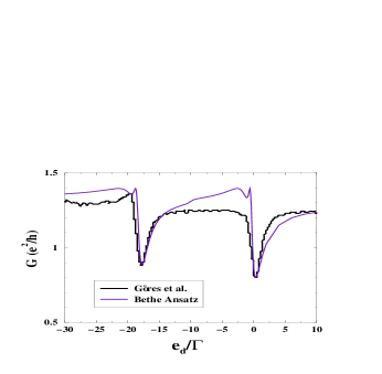
FIG. 1.: A plot describing the $T=0$ linear response conductance. The solid curve corresponds to that predicted by the Bethe ansatz given the parameters $\Gamma=.05U$, $V_{Ld}/V_{Rd}=.75$, and $\Theta=0.78$, while the circles correspond to experimental data reported for a pair of Fano resonances reported in Göres et al. [2].

We now determine the necessary parameters, $U$, $\Gamma$, $V_{dL/R}$, and $V_{LR}$ entering the model Hamiltonian. From the spacing of the peaks together with their widths, the ratio $\Gamma/U$ is given by $1/20$. To determine the values of $V_{Ld}/V_{Rd}$ and $V_{LR}$ we use the fact that $G$ for large values of the gate voltage tends to its $U=0$ value of $\gamma 4\Theta^{2}/(1+\Theta^{2})^{2}$, with $\gamma=4V_{dL}^{2}V_{dR}^{2}/\Gamma^{2}$ and $\Theta=V_{LR}/\sqrt{\gamma}$. Furthermore the value of $V_{LR}$ determines the depth of the dip in $G$. Using then only two data points we fix these later two parameters.

With these in hand, we manage to reproduce the linear response conductance for the entire span of both peaks (see Figure 1). We note that the data to which we compare our theoretical calculations was taken at a low but finite temperature. We expect the extremely sharp features seen in our $T=0$ computation to be washed out at this temperature.

A feature of these resonances is that $G$ never vanishes. In terms of our computation we believe this to be the result of our non-perturbative treatment of finite Coulomb interactions. In the free case $G(\epsilon_{d})=\gamma\sin^{2}(\tan^{-1}(\Theta-\Gamma/\epsilon_{d})+\tan^{-1}(\Theta))$ and $G$ vanishes for some $\epsilon_{d}$. Similarly the expression for $G$ arising out of the Dyson equations [10, 11] always vanishes for some value of $\epsilon_{d}$, one reason we suspect that the Dyson equations do not adequately capture the physics at finite $U$, $V_{LR}$. We also point out that the resonances occur for values of the gate voltage placing the dot in its mixed valence regime ($n_{d}<1$) and not the Kondo regime ($n_{d}\sim 1$). Generically, our solution predicts that the linear response conductance in the Kondo regime will be relatively structureless.

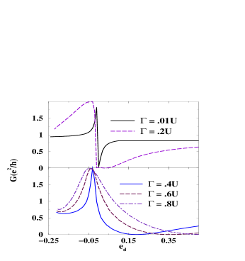
FIG. 2.: A set of Fano resonances for differing values of $\Gamma$. These curves are computed using $V_{LR}=0.4$.

Dependence of width of Fano resonances upon $\Gamma$: In [1], Fano resonances were studied as a function of the total dot-lead coupling strength, $\Gamma$, where it was observed that the width of Fano resonances exhibit a non-monotonic dependence upon $\Gamma$. (In a dot with a single tunneling path, the width of a resonance merely increases with $\Gamma$.) Together with this non-monotonicity, the overall shape and amount of asymmetry in the Fano resonances was observed to be sensitive to the strength of $\Gamma$.

We can reproduce this array of behaviour. Plotted in Figure 2 is the linear response conductance for a set of differing $\Gamma$’s. For $\Gamma$ small, a Fano resonance appears as a sharply peaked bipolar structure. As $\Gamma$ is increased, as naïvely expected, the bipolar peak broadens. However at some critical value of $\Gamma\sim(.3-.4)U$, the bipolar resonance is replaced by a narrow unipolar one. With further increases in $\Gamma$, this resonance proceeds to broaden out.

Linear response conductance at $H\neq 0$: The behaviour of Fano resonances in magnetic fields was also studied in [1]. It was found that the resonances exhibited a marked response to extremely small magnetic fields ($g\mu H/\Gamma\sim 10^{-2}$). In particular they demonstrated that upon application of $H$, a small bipolar Fano resonance is transformed into a much larger unipolar structure (see inset to Figure 3). We are able to reproduce this phenomena (see main body of Figure 3). For $H=0$, a small bipolar resonance in $G$ is present. With the introduction of a small field, a large unipolar peak is superimposed over the bipolar structure. As this calculation is done at $T=0$, finite T should lead the two structures to merge leaving a reasonable representation of the experimental data.

The strength of $H$ necessary to produce the unipolar peak is on the order of a putative Kondo temperature, $T_{k}$, which at the symmetric point of a single channel dot is estimated by, $T_{k}\sim\sqrt{U\Gamma}\exp(-U/8\Gamma)$. This might suggest that in applying $H$, a resonance (or lack thereof) due to the Kondo effect is destroyed.

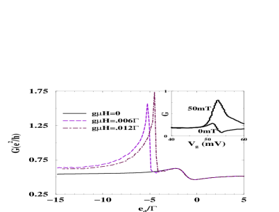
FIG. 3.: The response of a bipolar Fano resonance to the application of small magnetic fields, $H$. To compute these curves we employ $\Gamma/U=1/20$ and $V_{LR}=-3.6$. Inset: Observed response of a Fano resonance to small applied fields.

To summarize we have employed a generalized Anderson Hamiltonian to describe observations of Fano resonances in quantum dots. We have argued that this Hamiltonian is integrable and sketched how this integrability can be exploited to compute the $T=0$ linear response conductance. Using this model, we are able to describe a number of observed features of Fano resonances presented in [1]. Our exact solution of the model suggests that the physics underlying the resonances is non-perturbative in the presence of finite Coulomb repulsion on the dot.

The author acknowledges support from the NSF (DMR-9978074). He also acknowledges useful discussions with Aashish Clerk and David Goldhaber-Gordon.

REFERENCES

- [1] J. Göres, D. Goldhaber-Gordon, S. Heemeyer, M. A. Kastner, H. Shtrikman, D. Mahalu, and U. Meirav, Phys. Rev. B 62, 2188 (2000).
- [2] I. Zacharia, D. Goldhaber-Gordon, G. Granger, M. A. Kastner, Yu. Khavin, H. Shtrikman, D. Mahalu, and U. Meirav, Phys. Rev. B 64, 155311 (2001).
- [3] D. Goldhaber-Gordon, et al. cond-mat/9807233; D. Goldhaber-Gordon et al., Nature 391 (1998) 156.
- [4] S. Cronenwett, T. Oosterkamp, and L. Kouwenhoven, cond-mat/9804211; W.G. van der Wiel et al., Science 289, 2105 (2000); D.C. Ralph, R.A. Buhrman, PRL 72, 3401 (1994).
- [5] U. Fano, Phys. Rev. 124, 1866 (1961).
- [6] V. Madhavan, W. Chen, T. Jamneala, M. F. Crommie, and N. Wingreen, Science 280, 567 (1998).
- [7] O. Újsághy, J. Kroha, L. Szunyogh, and A. Zawadowski, PRL 85, 2557 (2000).
- [8] A. Yacoby, et al., PRL 74, 4047 (1995); K. Kobayashi et al., cond-mat/0202006.
- [9] A. Clerk et al., PRL 86, 4636 (2001).
- [10] B. Bulka et al., PRL 86 (2001) 5128.
- [11] W. Hofstetter et al., PRL 87, 156803 (2001).
- [12] D. Langreth, Phys. Rev. 150, 516 (1966).
- [13] P. Wiegmann et al., Sov. Phys. JETP Lett. 35 (1982) 77; N. Kawakami and A. Okiji, Phys. Lett. A 86 (1982) 483.
- [14] R. M. Konik, H. Saleur, and A.W.W. Ludwig, PRL 87, 236801 (2001); ibid, cond-mat/0103044, in press with PRB.
- [15] N. Andrei, Phys. Lett. A. 87 (1982) 299.