QUASICLASSICAL CALCULATION OF SPONTANEOUS CURRENT IN RESTRICTED GEOMETRIES

Calculation of current and order parameter distribution in inhomogeneous superconductors is often based on a self-consistent solution of Eilenberger equations for quasiclassical Green’s functions. Compared to the original Gorkov equations, the problem is much simplified due to the fact that the values of Green’s functions at a given point are connected to the bulk ones at infinity (boundary values) by “dragging” along the classical trajectories of quasiparticles. In finite size systems, where classical trajectories undergo multiple reflections from surfaces and interfaces, the usefulness of the approach is no longer obvious, since there is no simple criterion to determine what boundary value a trajectory corresponds to, and whether it reaches infinity at all. Here, we demonstrate the modification of the approach based on the Schophol -Maki transformation, which provides the basis for stable numerical calculations in 2D. We apply it to two examples: generation of spontaneous currents and magnetic moments in isolated islands of d-wave superconductor with subdominant order-parameters $s$ and $d_{xy}$, and in a grain boundary junction between two arbitrarily oriented d-wave superconductors. Both examples are relevant to the discussion of time-reversal symmetry breaking in unconventional superconductors, as well as for application in quantum computing.

1 Introduction

Pairing symmetry of unconventional superconductors can produce time-reversal symmetry breaking states. $\!{}^{{\bf?}}$ Especially interesting are high T_c cuprates, with their $d$-wave symmetry, since the recently developed technology $\!{}^{{\bf?}}$ allows fabrication of such structures, with controllable characteristics, as $\pi$-junctions, submicron size “$\phi_{0}$”-junctions $\!{}^{{\bf?}}$ (i.e. junctions with equilibrium phase difference $\phi_{0}$ which is neither 0 nor $\pi$), $\!{}^{{\bf?}}$ $\pi$-SQUIDs $\!{}^{{\bf?}}$ or $\pi/2$-SQUIDs, $\!{}^{{\bf?}}$ and superconducting qubit prototypes. $\!{}^{{\bf?}}$ Therefore, quantitative prediction of properties of such restricted systems becomes relevant not just from the theoretical point of view.

General approach to such calculations is based on Gorkov equations for Green’s functions of the superconductor. It is limited only by the applicability of BCS-like “mean field” description of the superconducting state. This description is now considered valid on the phenomenological level, $\!{}^{{\bf?}}$ independently from further developments in the first principles’ theory of high T_c superconductivity. Quasiclassical limit of these equations, Eilenberger equations, $\!{}^{{\bf?}}$ is strictly speaking valid only when $|\Delta|\ll E_{F},$. Unlike in conventional superconductors, this condition is not completely satisfied in high $T_{c}$ superconductors but is still a good approximation.

2 Quasiclassical Approach

We use the standard approach based on Eilenberger equations $\!{}^{{\bf?}}$ for quasiclassical Green’s functions

$${\bf v}_{F}\cdot\nabla\widehat{g}+[\omega\widehat{\tau}_{3}+\widehat{\Delta},\widehat{g}]=0,$$ (1)

with normalization condition $\widehat{g}^{\ 2}=\widehat{1}$, where $\omega$ is the Matsubara frequency and

$$\widehat{\tau}_{3}=\left(\begin{array}[]{cc}1&0\\ 0&-1\end{array}\right),\quad\widehat{g}=\left(\begin{array}[]{cc}g&f\\ f^{\dagger}&-g\end{array}\right),\quad\widehat{\Delta}=\left(\begin{array}[]{cc}0&\Delta\\ \Delta^{\dagger}&0\end{array}\right).$$

The matrix Green’s function $\widehat{g}$ and the superconducting order parameter $\Delta$ are both functions of the Fermi velocity ${\bf v}_{F}$ and position ${\bf r}$. $\Delta$ is determined by the (2D) self-consistency equation

$$\Delta(\theta)=2\pi N(0)T\sum\limits_{\omega>0}\left<V_{\theta\theta^{\prime}}f(\theta^{\prime})\right>_{\theta^{\prime}}$$

where $\theta$ is the angle between ${\bf v}_{F}$ and the $x$-axis, $V_{\theta\theta^{\prime}}$ interaction potential, $N(0)$ density of states at the Fermi surface, and $\left<...\right>_{\theta}$ represents averaging over $\theta$. Generally, it is possible to obtain a mixture of different symmetries of the order parameter, e.g. $\Delta=\Delta_{x^{2}-y^{2}}+\Delta_{xy}+\Delta_{s}$ where $\Delta_{x^{2}-y^{2}}=\Delta_{1}\cos 2\theta,$ $\Delta_{xy}=\Delta_{2}\sin 2\theta$, and $\Delta_{s}$ are the dominant $d_{x^{2}-y^{2}}$ component, and the subdominant $d_{xy}$ and the $s$ components of the order parameter respectively. The corresponding interaction potential, $V_{\theta\theta^{\prime}}=V_{d1}\cos 2\theta\cos 2\theta^{\prime}+V_{d2}\sin 2\theta\sin 2\theta^{\prime}+V_{s},$ must be substituted in the self-consistency equation. The current density ${\bf j(r)}$ is found from $g$ as

$${\bf j}=-4\pi ieN(0)T\sum\limits_{\omega>0}\left<{\bf v}_{F}g\right>_{\theta}$$

For numerical calculations, it is conventional $\!{}^{{\bf?},{\bf?},{\bf?}}$ to parameterize the quasiclassical Green’s functions by so called coherent functions $a,b$ via

$$g={\frac{1-ab}{1+ab}}\ ,\quad f={\frac{2a}{1+ab}}.$$ (2)

Functions $a$ and $b$ satisfy two independent, but nonlinear, equations

$${\bf v}_{F}\cdot\nabla a = \Delta-\Delta^{\ast}a^{2}-2\omega a$$

$$-{\bf v}_{F}\cdot\nabla b = \Delta^{\ast}-\Delta b^{2}-2\omega b.$$ (3)

From these equations it follows that $a(-{\bf v}_{F})=b^{\ast}({\bf v}_{F})$ and $b(-{\bf v}_{F})=a^{\ast}({\bf v}_{F})$. One should solve these equations along all possible quasiclassical trajectories and perform the summation over the trajectories to calculate the order parameter current density. To find $a$ and $b$ along the trajectories, one needs to use boundary conditions at the ends of the trajectories. In macroscopically large systems, one usually assumes that all the trajectories go deep into the bulk of the superconductor, i.e., it is possible to use the bulk solutions

$$a_{\pm}={\frac{\Delta}{\omega\pm\Omega}}\ ,\qquad b_{\pm}={\frac{\Delta^{\ast}}{\omega\pm\Omega}}$$ (4)

with $\Omega=\sqrt{\omega^{2}+|\Delta|^{2}}$, as the boundary conditions at infinity. In the case of “restricted” systems, the above assumption is no longer self-evident. Nevertheless, we will see that a stable numerical procedure can be still developed.

Numerical calculation is stable if the integration for $a$ ($b$) is taken in the (opposite) direction of ${\bf v}_{F}$. When $\Delta$ is a constant, the solution of Eq. (3) for $a$ is

$$a_{f} = a_{+}+{\frac{a_{i}-a_{+}}{1+{\frac{\Delta^{\ast}}{\Omega}}(a_{i}-a_{-})e^{\Omega\tau}\sinh\Omega\tau}}$$ (5)

$$\approx a_{+}+{\frac{\Omega}{\Delta^{\ast}}}\left({\frac{a_{i}-a_{+}}{a_{i}-a_{-}}}\right)e^{-2\Omega\tau},\quad{\rm for}\ \Omega\tau\gg 1$$

where $a_{i}$ and $a_{f}$ are the values of $a$ at the initial (${\bf r}_{i}$) and final (${\bf r}_{f}$) points of the trajectory, and $\tau=|{\bf r}_{f}-{\bf r}_{i}|/v_{F}$ is proportional to the distance between the initial and final points along the trajectory. It is clear that the solution for $a$ relaxes to the bulk value $a_{+}$ at the distance $L={\bf v}_{F}/2\Omega$ which is of the order of the coherence length $\xi_{0}$. In other words, when the quasiparticle moves away from the initial point at a distance of a few $\xi_{0}$’s, any information about the initial point $a_{i}$ becomes lost. This observation is also valid for $b$, and is crucial for what that follows.

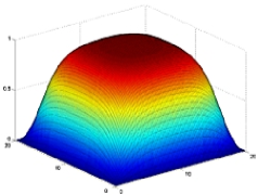
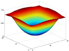
Figure 1: Absolute values of the dominant (left) and subdominant (right) order parameters for a small square $d$-wave super conductor in the presence of subdominant $s$-wave order parameter. The orientation of the main order parameter is $45^{\circ}$ rotated with respect to the boundaries.

Let us now specifically consider a restricted system. After integrating over a few $\xi_{0}$’s, $a_{f}$ will be almost independent of $a_{i}$, although it may never coincide with the bulk value $a_{+}$. This solution corresponds to a simple exponential relaxation of the functions $a$ and $b$ to their local “steady-state” values defined by the local value of the order parameter. This value is the limit for the functions $a$ and $b$ at this spatial point. Such relaxation of Green’s functions significantly simplifies the numerical solution of the self-consistent two-dimensional problem. The system therefore has no memory of the local values of $\Delta$ beyond several $\xi_{0}$ along the trajectory.

In order to calculate $a$, we define all possible trajectories going through a given point of the system. Along each of them we move back (in the direction opposite to ${\bf v}_{F}$) a cutoff distance (about $10\xi_{0}$– $20\xi_{0})$ and choose that point as the beginning of the trajectory. We set the bulk solution ($a_{+}$) as the initial value for $a$ at that point (this really does not matter too much because the system has no memory) and integrate along the trajectory, taking into account the reflections at the boundaries, until we get back to the calculation point. Calculation for $b$ is the same, except that the direction of integration is now opposite to ${\bf v}_{F}$. These calculations are repeated for all trajectories and all points of the system (on a mesh). After each iteration, we calculate the new $\Delta$ and use it for the next iteration until the self-consistency is achieved. We found this method to be very stable and independent of the value of the “cutting” distance. One should note that the above procedure is not valid in the presence of magnetic field, because a path dependent phase will be accumulated to the Green’s functions, and the above mentioned relaxation mechanism along the trajectory does not work anymore.

3 Results

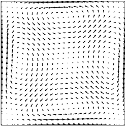
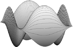
Figure 2: Spontaneous current density (left) and magnetic field distribution (right) for the system of Fig. 1.

To illustrate the approach, we performed self-consistent calculations of the order parameter in a small ($20\xi_{0}\times 20\xi_{0}$) square region of $d$-wave superconductor in the presence of a subdominant $s$-wave order parameter. The crystalographic $a$ and $b$ directions of the dominant order parameter make $45^{\circ}$ angle with respect to the boundaries of the square. We used a random subdominant order parameter at the first iteration in order to avoid imposing any assumption on the phase of the second order parameter.

The two components of the order parameter are displayed in Fig. 1. The dominant order parameter is suppressed at the boundaries of the square. This is due to the special orientation of the order parameter which requires all quasiparticles to face opposite sign of the order parameter after reflecting from the boundaries. $\!{}^{{\bf?}}$ As a result, the subdominant order parameter ($s$) with a $\pi/2$ phase shift with respect to the dominant order parameter, is the main contributor at the boundaries. The spontaneous current distribution is displayed in Fig. 2. The current does not flow in the same direction at all the four edges, but changes the direction from one edge to another closing its path towards the center of the square. The magnetic field produced by the current is also shown in Fig. 2. The maximum value of the magnetic field is of the order of $10^{-3}G$. Notice that the direction of the filed changes from one edge to another. Thus, the total flux produced by such a field is zero.

We also have calculated the spontaneous current and magnetic field distributions in a $d$-wave grain boundary junction. The system consists of a finite square ($30\xi_{0}\times 30\xi_{0}$) made of $d$-wave superconductor divided into two equal parts separated by a grain boundary junction. The order parameter has $d_{x^{2}-y^{2}}$ symmetry with $0^{\circ}$ orientation on the left side of the grain boundary and $45^{\circ}$ on the right side. We include a $d_{xy}$ subdominant order parameter by adding an attraction potential in that channel (see Ref. $\!{}^{{\bf?}}$). The magnitude of potential is chosen in such a way to have a transition temperature $T_{c2}=0.1T_{c}$ (in the absence of the dominant order). $\!{}^{{\bf?}}$ We choose a phase difference of $\Delta\phi=\pi/2$ between the two sides. This actually corresponds to the equilibrium phase difference of the junction at which the total current passing through the junction is zero. $\!{}^{{\bf?}}$ Calculations are done at $T=0.05T_{c}$.

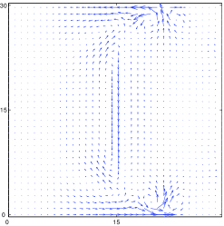
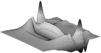
Figure 3: Absolute value of the order parameter for a grain boundary junction between two d-wave superconductors. The grain boundary is a vertical line located in the middle. The orientation of the order parameter is $0^{\circ}$ on the left and $45^{\circ}$ on the right.

The results of calculation of the spontaneous current and magnetic field distributions are displayed in Fig. 3. Notice that the current is not symmetric with respect to the grain boundary. On the left side (with $0^{\circ}$ orientation), the current returns along the diagonal, whereas on the right side ($45^{\circ}$ orientation) it forms two vortices and antivortices near the edges. These vortices are a consequence of the chiral nature of the $d+id^{\prime}$ symmetry. $\!{}^{{\bf?},{\bf?}}$ Magnetic field is peaked at the location of vortices with a maximum of the order of $10^{-3}G$. It is important to emphasize that, unlike in the previous case, the existence of the spontaneous current in this system does not depend on the presence of a subdominant order parameter (although we assumed a subdominant component here). Addition of a subdominant order parameter will actually suppress the spontaneous current at the boundary (see Refs. $\!{}^{{\bf?},{\bf?}}$).

4 Conclusions

We described a method to calculate equilibrium properties in finite size superconducting systems. We presented the results of our calculations for the distribution of spontaneous current and magnetic field in two systems: a small square region of a $d$-wave superconductor with a pair breaking boundary, and a $d$-wave grain boundary junctions between two differently oriented $d$-wave superconductors. The method described here is quite general and can be applied to any 2D geometry with proper boundary conditions. Presence of external magnetic field invalidates the method described here. The self-generated magnetic field due to the spontaneous currents, however, is usually very small so that its effect can be neglected in most calculations.

References

References

- [1] M. Sigrist, Prog. Theo. Phys. 99, 899 (1998); D.J. Scalapino, Phys. Rep. 250, 330 (1995).
- [2] A.Yu. Tzalenchuk, et al., preprint.
- [3] E. Il’ichev, et al. Phys. Rev. Lett. 86, 5368 (2001).
- [4] M.H.S. Amin, A.N. Omelyanchouk, S.N. Rashkeev, M. Coury, and A.M. Zagoskin, Physica B, in press (cond-mat/0105486).
- [5] R.R. Schulz, et al., Appl. Phys. Lett. 76, 912 (2000).
- [6] M.H.S. Amin, M. Coury, and G. Rose, IEEE Trans. Appl. superconductivity, in press (cond-mat/0107370).
- [7] L.B. Ioffe, et al., Nature 398, 679 (1999); A. Blais and A.M. Zagoskin, Phys. Rev. A 61, 042308 (2000).
- [8] V.P. Mineev and K.V. Samokhin, Introduction to unconventional superconductivity, Gordon and Breach Science Publishers (1999).
- [9] G. Eilenberger, Z. Phys. 214, 195 (1968).
- [10] M.H.S. Amin, A.N. Omelyanchouk, and A.M. Zagoskin, Phys. Rev. B 63, 212502 (2001).
- [11] N. Schopohl and K. Maki, Phys. Rev. B 52, 490 (1995); N. Schopohl, preprint (cond-mat/9804064).