Activation energies for spin reversed excitations in the fractional quantum Hall effect

Abstract

The activation energy measured in transport experiments in the fractional Hall regime corresponds to the energy required to create a far separated particle hole pair. We calculate, for several fractional quantum Hall states, the energy gap for the excitation in which the excited composite fermion reverses its spin quantum number. We consider an ideal system with zero thickness as well as the more realistic quantum well geometry, while neglecting Landau level mixing and disorder, and find that the spin reversed excitations may be relevant for experimentally accessible parameters.

The phenomenon of the fractional quantum Hall effect (FQHE) [1] occurs because of the opening up of gaps at certain fractional filling factors, measured experimentally by studying the temperature dependence of the longitudinal resistance [2, 3, 4, 5]). While the gaps at the integral fillings appear due to the well known quantization of the kinetic energy into Landau levels, the FQHE gaps owe their origin to inter-electron interaction and signify the appearance of a collective state. This remarkable correlated state with extraordinary properties is described in terms of particles called composite fermions, namely electrons bound to an even number of vortices [6]. The composite fermions experience a reduced effective magnetic field, and have an effective filling factor $\nu^{*}$, which is related to the electron filling factor $\nu$ by $\nu=\nu^{*}/(2p\nu^{*}\pm 1)$. The formation of composite fermions gives a simple intuitive explanation for the existence of the gaps. A gap opens up when the composite fermions occupy an integral number of their Landau levels (called composite-fermion Landau levels), i.e., when $\nu^{*}=n$, which gives FQHE at $\nu=n/(2pn\pm 1)$, precisely the observed sequences of fractions.

In addition to the above intuitive understanding, the composite fermion theory gives an accurate microscopic description. Wave functions for the ground state and the excitations [6] are known, from comparisons with exact results obtained in numerical diagonalization studies on finite systems, to be practically identical to the exact wave functions [7]. In particular, they produce energy gaps with an accuracy of a few percent. The energy gaps have been calculated for several FQHE states for a strictly two-dimensional electron system with no disorder and no Landau level mixing (referred to as the “ideal” system below) [8, 9, 7], and corrections due to finite thickness and Landau level mixing have also been estimated [10, 11, 12, 13]. While the theory obtains the qualitative trends seen experimentally [4, 5], there still are significant quantitative disagreements between the theoretical and experimental gaps [12]. Because the composite fermion (CF) theory gives an accurate account of the computer experiments on the ideal system, it is believed that the discrepancy between theory and experiment is caused by the approximate theoretical treatment of the finite thickness and Landau level mixing effects, and also because of the ever present disorder.

This article reports results on the energy gaps to spin reversed excitations. The gap to creating a spin reversed excitation was studied for $\nu=1/3$ prior to the composite fermion theory in exact diagonalization studies [14, 15], and it was estimated that for the ideal system, the energy of the spin reversed excitation is $\Delta^{\uparrow\downarrow}=\Delta_{C}^{\uparrow\downarrow}+\Delta_{Z}$, with $\Delta_{C}^{\uparrow\downarrow}=0.075V_{C}$ as opposed to the energy of the excitation that does not involve spin reversal $\Delta^{\uparrow\uparrow}=0.105V_{C}$. Here $\Delta_{Z}$ is the Zeeman splitting, and the interaction component is measured in units of $V_{C}={e^{2}\over\epsilon l}$ where $l=\sqrt{\hbar c/eB}$ is the magnetic length and $\epsilon$ is the background dielectric constant. For GaAs, with the magnetic field quoted in Tesla and the energies in Kelvin, we have $V_{C}=50\sqrt{B[T]}$ K and $\Delta_{Z}=0.30B[T]$ K, and the above result implies that for magnetic fields below $B_{c}\approx 28$T, the observed gap at $\nu=1/3$ corresponds to the spin reversed excitation. However, early experimental studies [16] indicated otherwise. As we shall see, the crossover magnetic field is a very sensitive function of various parameter; the modification of the interaction due to the finite width of the actual experimental system significantly diminishes the value of the crossover magnetic field and the fully polarized excitation becomes relevant for typical parameters.

At first sight, it may seem surprising that the interaction energy of the spin reversed excitation is less than that of fully polarized excitation, because a reasoning based on exchange energy considerations would point toward quite the opposite conclusion. The explanation is that more important than exchange energy is the effective Landau level (LL) energy of composite fermions: $\Delta^{\uparrow\uparrow}$ involves transition of a composite fermion into a higher CF LL, whereas $\Delta^{\uparrow\downarrow}$ does not. We consider here spin reversed excitations at general filling factors of the form $\nu=n/(2n+1)$. The difference from $n=1$ case ($\nu=1/3$) is the possibility of transitions into lower CF Landau levels, which might make spin reversed excitations more favorable. Our results indicate that spin reversed excitations may be more pervasive than thought earlier; the gaps at 3/7 and 4/9 may actually correspond to spin reversed excitations for typical experiments.

FIG. 1.: Schematic depiction of a particle hole pair of composite fermions at $\nu^{*}=3$ ($\nu=3/7$), with composite fermions shown as electrons bound to two flux quanta. The figure to the left of the vertical dashed line shows the spin conserving excitation, and the figure on the right shows the excitation in which a composite fermion falls into a lower spin reversed CF Landau level. The label at the the side of each CF Landau level, e.g., $2\uparrow$ or $1\downarrow$ gives the CF-LL index along with the spin. The Zeeman splitting is neglected for simplicity.

We compute the gaps following the method outlined in detail in the literature [7, 12], using the spherical geometry [17] which considers $N$ electrons on the surface of a sphere, moving under the influence of a strong radial magnetic field. The wave function for the ground state is given by $\Psi_{n/(2n+1)}={\cal P}_{LLL}\Phi_{n}\Phi_{1}^{2}$, where $\Phi_{n}$ is the wave function of the $n$ filled LL state, and ${\cal P}_{LLL}$ is the lowest LL projection operator. The ground state will be taken to be fully spin polarized. The wave function for the excited state is $\Psi^{\uparrow\downarrow}_{n/(2n+1)}={\cal P}_{LLL}\Phi^{\uparrow\downarrow}_{n}\Phi_{1}^{2}$, where $\Phi^{\uparrow\downarrow}_{n}$ is the wave function of that excited state at $\nu=n$ in which one particle has been removed from the highest occupied spin-up Landau level and placed in the lowest spin-down Landau level. The state $\Psi^{\uparrow\downarrow}_{n/(2n+1)}$ is then interpreted as the state in which one composite fermions has transferred from highest occupied spin-up CF-LL to the lowest spin-down CF-LL, as shown in Fig. (1). We are interested in the energy of this excitation in limit that the distance between the CF particle and the CF hole is very large, so we consider the excited state in which they are on the opposite poles of the sphere. We compute the energy gaps by evaluating the expectation values of the interaction energy ${\hat{V}}=\sum_{j<k}V(r_{jk})$ in the composite fermion wave functions for the ground and excited states:

$$\Delta_{C}^{\uparrow\downarrow}=\frac{<\Psi^{\uparrow\downarrow}_{n\over 2n+1}|{\hat{V}}|\Psi^{\uparrow\downarrow}_{n\over 2n+1}>}{<\Psi^{\uparrow\downarrow}_{n\over 2n+1}|\Psi^{\uparrow\downarrow}_{n\over 2n+1}>}-\frac{<\Psi_{n\over 2n+1}|{\hat{V}}|\Psi_{n\over 2n+1}>}{<\Psi_{n\over 2n+1}|\Psi_{n\over 2n+1}>}.$$

The expectation value of the interaction requires evaluation of multidimensional ($2N$-dimensional) integrals, which is accomplished by Monte Carlo for different numbers of particles, and the thermodynamic limit is obtained as shown in Fig. (2). (Prior to an extrapolation of our results to the limit of $N\rightarrow\infty$, we correct for the interaction between the CF particle and the CF hole, which amounts to a subtraction of $-(2n+1)^{-2}/2\epsilon R$, the interaction energy for two point-like particles of charges $e/(2n+1)$ and $-e/(2n+1)$ at a distance $2R$, where $R$ is the radius of the sphere. We also correct for a finite size deviation of the density from its thermodynamic value, by multiplying by a factor $\sqrt{\rho/\rho_{N}}$, where $\rho$ is the thermodynamic density and $\rho_{N}$ is the density of the $N$ particle system.) For the ideal system with zero thickness, we use $V(r)=e^{2}/\epsilon r$ to obtain the gaps. For the more realistic situation, we calculate the profile of the transverse wave function within a local density approximation[18], and integrate over the transverse coordinate produces an effective two-dimensional interaction. The details of the calculation as well as of various approximations made have been outlined in Ref. [12].

FIG. 2.: The determination of the thermodynamic limit by extrapolation of finite system results for the quantum well system of width 20nm with electron density $\rho=1.0\times 10^{11}$ cm^-2. A linear fit is assumed. The error bars show the statistical uncertainty in the Monte Carlo evaluation of the energy gap. $N$ is the number of particles, and the energies are given in units of $e^{2}/\epsilon l$, where $l$ is the magnetic length and $\epsilon$ is the dielectric constant of the background material.

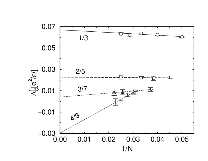
The thermodynamic values for the interaction component of the gaps for the ideal system are given in Table I for several filling factors. A comparison with $\Delta^{\uparrow\uparrow}$, calculated earlier [12] and reproduced in Table I, produces rather large values for the crossover magnetic field, $B_{c}$, below which the lowest energy gap involves spin reversal. At filling factor $\nu$, the magnetic field is related to the density as $\rho=(\nu B[T]/3.9)\times 10^{11}$cm^-2, from which the densities can be obtained below which the gap corresponds to excitation of a spin reversed composite fermion.

Whether the activation gap corresponds to $\Delta^{\uparrow\downarrow}$ or $\Delta^{\uparrow\uparrow}$ depends on whether the ratio $\Delta^{\uparrow\downarrow}/\Delta^{\uparrow\uparrow}$ is smaller or larger than one. As the CF filling $n$ increases, there are two competing effects. First, the magnitude of the interaction components of the gaps are expected to decrease, which would increase the ratio $\Delta^{\uparrow\downarrow}/\Delta^{\uparrow\uparrow}$ and suppress spin reversal. On the other hand, in creating a spin reversed excitation, the composite fermion can jump down by more CF-Landau levels for larger $n$, thereby leading to a larger decrease in the interaction energy relative to the fully polarized excitation, which would decrease the ratio. Our microscopic calculation shows that the latter effect wins, at least for the ideal situation.

$\nu$	$\Delta_{C}^{\uparrow\downarrow}=\Delta^{\uparrow\downarrow}-\Delta_{Z}$ [${e^{2}\over\epsilon l}$]	$\Delta^{\uparrow\uparrow}$ [${e^{2}\over\epsilon l}$]	$B_{c}$[T]	$B_{tr}$[T]
1/3	0.0740(24)	0.106(3)	28	-
2/5	0.0235(55)	0.058(5)	33	3.5
3/7	0.0022(94)	0.047(4)	56	5.8
4/9	$-0.0402(135)$	0.035(6)	157	7.4

TABLE I.: The interaction components of the lowest excitation gaps involving spin reversal ($\Delta_{C}^{\uparrow\downarrow}=\Delta^{\uparrow\downarrow}-\Delta_{Z}$) and no spin reversal $\Delta^{\uparrow\uparrow}$. The magnetic field is quoted in Tesla and the energy is quoted in units of $e^{2}/\epsilon l$, where $l$ is the magnetic length and $\epsilon$ is the dielectric constant of the background material. The results are for $V(r)=e^{2}/\epsilon r$, as appropriate for a system with zero thickness; Landau level mixing and disorder are not considered. The crossover magnetic field $B_{c}$ is given for parameters appropriate for GaAs; the spin reversed excitation has the lowest energy for fields below $B_{c}$. Also given is the magnetic fields $B_{tr}$, at which a transition into a partially polarized ground state takes place. The gaps $\Delta_{C}^{\uparrow\uparrow}$ are taken from Jain and Kamilla [7], $B_{tr}$ from Park and Jain [21], and the value of $\Delta_{C}^{\uparrow\downarrow}$ for $\nu=1/3$ is consistent with that of Rezayi [15].

Our calculation above assumes a fully polarized ground state, but it is well known, from numerical diagonalization studies [19], from the composite fermion theory [20, 21], and also experimentally [22, 23], that for sufficiently small Zeeman energies, the FQHE ground state is not fully polarized. The fully polarized state at $\nu^{*}=n$, denoted by $(n,0)$, makes a transition into the state $(n-1,1)$, which has $n-1$ spin-up and 1 spin-down CF-LLs occupied, as the Zeeman energy is reduced. Because a fraction $1/n$ of the total number of particles reverses its spin at the transition, the magnetic field $B_{tr}$ at the transition is determined from the equation $E_{C}^{(n,0)}-E_{C}^{(n-1,1)}=\Delta_{Z}/n$, where $E_{C}$ is the interaction energy per particle. For the ideal case, the energy differences[21] $E_{C}^{(n,0)}-E_{C}^{(n-1,1)}$ for $\nu^{*}=2$, 3, and 4 are 0.0056, 0.0048, 0.0041 in units of $V_{C}$, with the resulting $B_{tr}$ given in Table I. There is a range of magnetic fields with $B_{tr}<B<B_{c}$ where the ground state is fully polarized but the lowest energy excitation involves spin reversal.

These numbers might suggest that the gap to spin reversed excitation is the relevant gap for GaAs for almost all of the experimental range of parameters. That is not the case, however, because $B_{c}$ is a sensitive function of certain features left out in the ideal model. We consider now the finite thickness corrections, that will reduce the interaction components of both $\Delta^{\uparrow\downarrow}$ and $\Delta^{\uparrow\uparrow}$, but leave the Zeeman contribution to $\Delta^{\uparrow\downarrow}$ unaffected. The calculated gaps are given in Fig. (3) for quantum well widths 20 and 30 nm as a function of the density. The crossover magnetic fields are lowered compared to the ideal case, but are still in experimentally accessible regime for all of the filling factors considered.

FIG. 3.: The energies of spin reversed (thick lines) and spin polarized (thin lines) excitations, in Kelvin, for several filling factors, as a function of the electron density, for quantum wells of widths 20 nm (solid lines) and 30 nm (dashed lines). The gaps include the Zeeman contribution, wherever appropriate; the gap $\Delta^{\uparrow\downarrow}$ at $\nu=3/7$ is essentially equal to the Zeeman energy because of the smallness of the Coulomb contribution, $\Delta_{C}^{\uparrow\downarrow}$. The typical Monte Carlo uncertainty is shown at the left. The energies of the spin polarized excitations are taken from Park, Meskini, and Jain [12].

As is clear in the above, the crossover magnetic field is a sensitive function of the difference between the gaps, and a reliable estimation of its value would require an accurate quantitative understanding of the observed gaps, which is not available at the present. The treatment of finite thickness is reliable only on the order of 20% for each individual gap. Also, we have not considered in this work the effect of LL mixing [24], which further modifies the gap, perhaps by 10-20% for typical experimental parameters. Even after both the finite thickness and LL mixing corrections are included in the theory, the actual values of the theoretical and experimental gaps are off by approximately a factor of two [12], presumably because of disorder. Due to the unsatisfactory quantitative understanding of the observed gaps, it is not possible to say how trustworthy our estimates of $B_{c}$ are insofar as the actual experiments are concerned, but the qualitative trends found in our study ought to be robust.

This work was supported in part by the National Science Foundation under grant no. DMR-9986806.

REFERENCES

- [1] D.C. Tsui, H.L. Stormer, and A.C. Gossard, Phys. Rev. Lett. 48, 1559 (1982).
- [2] A.M. Chang et al., Phys. Rev. B 28, 6133 (1983).
- [3] R.L. Willett et al., Phys. Rev. B 37, 8476 (1988).
- [4] R.R. Du, H.L. Stormer, D.C. Tsui, L.N. Pfeiffer, and K.W. West, Phys. Rev. Lett. 70, 2944 (1993).
- [5] H.C. Manoharan, M. Shayegan, and S.J. Klepper, Phys. Rev. Lett. 73, 3270 (1994).
- [6] J.K. Jain, Phys. Rev. Lett. 63, 199 (1989); Phys. Rev. B 41, 7653 (1990); Physics Today 53(4), 39 (2000).
- [7] J.K. Jain and R.K. Kamilla, Int. J. Mod. Phys. B 11, 2621 (1997); Phys. Rev. B 55, R4895 (1997).
- [8] F.D.M. Haldane and E.H. Rezayi, Phys. Rev. Lett. 54, 237 (1985).
- [9] G. Fano, F. Ortolani, and E. Colombo, Phys. Rev. B 34, 2670 (1986).
- [10] F.C. Zhang and S. Das Sarma, Phys. Rev. B 33, 2903 (1986).
- [11] D. Yoshioka, J. Phys. Soc. Jpn. 55, 885 (1986).
- [12] K. Park, N. Meskini, and J.K. Jain, J. Phys. Condens. Mat. 11, 7283 (1999).
- [13] G. Murthy and R. Shankar, Phys. Rev. B 59, 12260 (1999).
- [14] T. Chakraborty, P. Pietilainen, and F.C. Zhang, Phys. Rev. Lett. 57, 130 (1986).
- [15] E.H. Rezayi, Phys. Rev. B 36, 5454 (1987).
- [16] J. E. Furneaux, D. A. Syphers, A. G. Swanson, Phys. Rev. Lett. 63, 1098 (1989)
- [17] F.D.M. Haldane, Phys. Rev. Lett. 51, 605 (1983).
- [18] F. Stern and S. Das Sarma, Phys. Rev. B 30, 840 (1984); S. Das Sarma and F. Stern, ibid. B 32, 8442 (1985); M.W. Ortalano, S. He, and S. Das Sarma, Phys. Rev. B 55, 7702 (1997).
- [19] F.C. Zhang and T. Chakraborty, Phys. Rev. B 30, 7320 (1984); 29, 7032 (1984); P. Maksym, J. Phys. C 1, 6299 (1989); X.C. Xie, Y. Guo, and F.C. Zhang, Phys. Rev. B 40, 3487 (1989).
- [20] X.G. Wu, G. Dev, and J.K. Jain, Phys. Rev. Lett. 71, 153 (1993);
- [21] K. Park and J.K. Jain, Phys. Rev. Lett. 80, 4237 (1998); Solid State Commun. in press.
- [22] R.G. Clark et al., Phys. Rev. Lett. 62, 1536 (1989); J.P. Eisenstein et al., ibid., 62, 1540 (1989); Phys. Rev. B 41, 7910 (1990); L.W. Engel et al., ibid., 45, 3418 (1992); W. Kang et al., Phys. Rev. B 56, 12776 (1997).
- [23] R.R. Du et al., Phys. Rev. Lett. 75, 3926 (1995); Phys. Rev. B 55, R7351 (1997); R.J. Nicholas et al. Semicond. Sci. Technol. 11, 1477 (1996).
- [24] D. Yoshioka, J. Phys. Soc. Jpn. 53, 3740 (1984); X. Zhu and S.G. Louie, Phys. Rev. Lett. 70, 339 (1993).