Ordering kinetics in an fcc $A_{3}B$ binary alloy model: Monte Carlo studies.

Abstract

Using an atom–vacancy exchange algorithm, we investigate the kinetics of the order–disorder transition in an fcc $A_{3}B$ binary alloy model following a temperature quench from the disordered phase. We observe two clearly distinct ordering scenarios depending on whether the final temperature $T_{f}$ falls above or below the ordering spinodal $T_{sp}$, which is deduced from simulations at equilibrium. For shallow quenches ($T_{f}>T_{sp}$) we identify an incubation time $\tau_{inc}$ which characterizes the onset of ordering through the formation of overcritical ordered nuclei. The algorithm we use together with experimental information on tracer diffusion in Cu₃Au alloys allows us to estimate the physical time scale connected with $\tau_{inc}$ in that material. Deep quenches, $T_{f}<T_{sp}$, result in spinodal ordering. Coarsening processes at long times proceed substantially slower than predicted by the Lifshitz–Allen–Cahn $t^{1/2}$ law. Structure factors related to the geometry of the two types of domain walls that appear in our model are found to be consistent with Porod’s law in one and two dimensions.

I Introduction

Several face–centered cubic binary metallic alloys, like Cu₃Au, Cu₃Pd, Mg₃In, Co₃Pt, etc. exhibit long range order with a $L1_{2}$–structure below some specific ordering temperature $T_{0}$. In the $L1_{2}$–structure four equivalent phases exist, where one of the four simple cubic sublattices building the fcc–lattice are preferentially occupied by the minority atoms. In studying kinetic processes of phase ordering, the following general considerations must be taken into account:

1. The transition is of first order. Hence, for small enough supercoolings the disordered phase remains metastable. Relaxation at short times after a temperature quench is governed by the formation of ordered nuclei, which grow into the disordered matrix. On the other hand, the concept of spinodal ordering has been advanced AllenCsp to characterize the phase ordering processes under large supercoolings.

2. The degeneracy of the ordered phase implies a four–component order parameter, $\Psi=(\psi_{0},\psi_{1},\psi_{2},\psi_{3})$. Here, $\psi_{\alpha}$ with $\alpha=1,2,3$, are non–conserved structural order parameter components coupled to a conserved density, $\psi_{0}$, which describes the concentration of the two atomic species.

3. The antiphase domain structure is anisotropic as a result of the existence of two types of antiphase domain walls: low–energy (type–I) and high–energy (type–II) walls.

Under these conditions a rich spectrum of kinetic processes is to be expected. In particular, there remain still open questions concerning scaling and universality in the late–stage growth kinetics. This has motivated several experimental investigations of ordering after a temperature quench, mostly on Cu₃Au, where direct information has been obtained from time–resolved X–ray diffraction and neutron scattering. On the other hand, only few theoretical or computer simulation studies on such materials have been reported so far .Lai ; Fron ; paper1 Frontera et al. Fron have recently simulated the growth of $L1_{2}$–ordered domains both within an atom–atom exchange and the more realistic atom–vacancy exchange mechanisms, for quench temperatures below the expected spinodal temperature $T_{sp}$. A similar model with atom–vacancy exchange ($ABV$–model) was applied by Kessler et al. paper1 to surface–induced kinetic ordering processes near Cu₃Au(001).

In this paper we investigate the ordering kinetics in the bulk of such alloys at quench temperatures $T_{f}$ both below and above $T_{sp}$. In contrast to earlier Monte Carlo studies of nucleation in Ising–type models BindStauf ; StaufferA we again employ the $ABV$–model with effective chemical interactions between nearest neighbors on the fcc–lattice. This allows us to compare our results directly with experiments on fcc–alloys, where vacancy–driven processes prevail. In particular, we analyze the nucleation regime, where we find a well defined incubation time that sensitively depends on the depth of the quench, $T_{0}-T_{f}$. Moreover, for $T_{f}<T_{sp}$, with $T_{sp}$ deduced from static correlations, we observe domain patterns typical to spinodal ordering. In the long–time coarsening regime we extract anisotropic scaling functions. Our model is a limiting case where type-I domain walls have exactly zero formation–energy and therefore are extremely stable. Within our accessible time window we find coarsening exponents which are significantly smaller than the conventional exponent $\alpha=1/2$ for curvature–driven coarsening.Lifsh ; AllenC

After shortly explaining our model and simulation techniques in section II, we compare in section III ordering processes that occur for shallow ($T_{0}>T_{f}>T_{sp}$) and deep ($T_{f}<T_{sp}$) quenches. In section IV we define the incubation time $\tau_{inc}$ and investigate its dependence on the depth of the quench. Anisotropic scaling functions are discussed in section V, while section VI contains a short summary of our results.

II Model and simulation method

We consider a three-dimensional lattice of $L\times L\times L$ fcc–cells with cubic lattice constant $a$ and periodic boundary conditions in all directions. Unless otherwise stated, we use $L=128$. Each site, $i$, of the lattice is occupied either by an atom of type $A$, an atom of type $B$, or a vacancy, with an obvious condition that the corresponding occupation numbers fulfill $c^{A}_{i}+c^{B}_{i}+c^{V}_{i}=1$. In accord with the stoichiometry of the $A_{3}B$ alloys there are exactly three times as many $A$ atoms present as $B$ atoms. The number of vacancies is chosen small enough so that they do not affect static properties of the system.

In our simplified model paper1 only nearest neighbor atom–atom interactions are taken into account. The corresponding Hamiltonian then reads:

$$H=\sum_{\langle i,j\rangle}[V_{AA}c^{A}_{i}c^{A}_{j}+V_{BB}c^{B}_{i}c^{B}_{j}+V_{AB}(c^{A}_{i}c^{B}_{j}+c^{B}_{i}c^{A}_{j})],$$ (1)

where the sum is restricted to nearest–neighbor pairs. We are interested here in the transition to the ordered $L1_{2}$–structure in which minority atoms ($B$) predominantly occupy one of the simple–cubic sublattices of the original fcc–lattice. It is then natural to assume $V_{BB}>0$, $V_{AA}<0$ and $V_{AB}<0$. The ground state of the $L1_{2}$ phase is fourfold degenerate and corresponds to all $B$–atoms segregated to exactly one of the simple cubic sublattices. For a stoichiometric $A_{3}B$-alloy the transition occurs at a temperature $T_{0}\simeq 1.83|J|/k_{B}$, with $J=-\frac{1}{4}(V_{AA}+V_{BB}-2V_{AB})$ as discussed in Ref. paper1, (cf. also Refs. Bind1, ; SchwL, ; Fron, ). The ordered phase is characterized by one conserved, scalar order parameter, $\psi_{0}$, related to the composition and three non–conserved order parameter components $(\psi_{1},\psi_{2},\psi_{3})$. These are defined by the following equations:

$$\psi_{0}=m_{1}+m_{2}+m_{3}+m_{4},$$

$$\psi_{1}=m_{1}-m_{2}-m_{3}+m_{4},$$

$$\psi_{2}=m_{1}-m_{2}+m_{3}-m_{4},$$ (2)

$$\psi_{3}=m_{1}+m_{2}-m_{3}-m_{4},$$

where $m_{\alpha}$ are the differences of the mean $A$– and $B$–occupation numbers, $m_{\alpha}=\langle{c^{A}_{i}}\rangle-\langle{c^{B}_{i}}\rangle$ for $i\in\alpha$. The index $\alpha=1\dots 4$ enumerates the four equivalent simple–cubic sublattices of the fcc–structure. For a homogeneous $A_{3}B$ alloy, $\psi_{0}=2$. In the disordered phase, $\psi_{1}=\psi_{2}=\psi_{3}=0$, while the four equivalent ordered phases are described as $(\psi_{1},\psi_{2},\psi_{3})/\bar{\psi}$ = $(-1,1,1)$; $(1,-1,1)$; $(1,1,-1)$ and $(-1,-1,-1)$, with a temperature–dependent $\bar{\psi}$ ($\bar{\psi}=2$ at $T=0$). For a non–homogeneous system Eq. (2) gives the corresponding local order parameters for each (cubic) elementary fcc–cell in terms of weighted averages of the occupation numbers computed of all sites belonging to the cell. (The weights are taken as the inverse of the numbers of neighboring fcc–cells that “share” the site in question, i. e. functions 1/2 and 1/8 are taken for the “face” and “corner” sites, respectively).

As can be seen from Eq. (2), each of the non–conserved components of the order parameter describes a modulation of the $B$–atom concentration along one of the cubic axes. For example, $\psi_{1}\neq 0$ means that the system contains alternating $B$–enhanced and $B$–depleted atomic layers along the $x$-axes. As a consequence of such layerwise arrangement of $B$–atoms, the (100) peak shows up in an X–ray diffraction experiment in addition to the (200), (020), (002) and (111) peaks characteristic of the underlying fcc–lattice. Similarly, $\psi_{2}$ and $\psi_{3}$–type ordering leads to additional (010) and (001) peaks, respectively.Warren For a distance $\vec{k}$ from these superstructure peaks the scattering intensity is described by the structure factors,

$$S_{\alpha}(\vec{k},t)=\langle{|\Psi_{\alpha}(\vec{k},t)|^{2}}\rangle,$$ (3)

which in a non–equilibrium state depend on time $t$. In Eq. (3), $\Psi_{\alpha}(k_{x},k_{y},k_{z},t)$ denotes the Fourier transform of the order parameter $\psi_{\alpha}(x,y,z,t)$, and $\alpha=1,2,3$. The widths of these intensity profiles are determined by the sizes of antiphase domains.Warren As mentioned in the Introduction, this system displays two types of antiphase boundaries, low–energy type–I boundaries with no change in the arrangement of nearest neighbors, and high–energy type–II boundaries.KikuchiC Since the Hamiltonian, Eq. (1), involves only nearest neighbor interactions, type–I boundaries in fact have zero energy.degeneracy

We assume here that the time–evolution of our model occurs only through atom–vacancy exchange processes. In an elementary move we first randomly single out one of the vacancies and, second, we choose at random one of its nearest neighbors occupied by an atom. The standard Metropolis algorithm is then used to decide whether the atom–vacancy exchange for the chosen pair takes place or not. In one Monte Carlo step (MCS), the system completes a series of as many such elementary moves as there are lattice sites in the system, i. e. $4L^{3}$, so that this time unit does not depend on the actual number of vacancies.

In previous simulations paper1 we have chosen the interaction parameters such that they were consistent with the observed Au–segregation at the Cu₃Au (001)–surface. Following Ref. paper1, , we take $V_{BB}=-V_{AA}=-V_{AB}>0$ and assume $c^{V}\simeq 6.1\cdot 10^{-6}$ as the mean density of vacancies present in the system.vacancy For vacancy concentrations of that order we have verified that both static and kinetic properties are independent of the precise value of $c^{V}$. To simulate a sudden quench from high temperatures to a final temperature $T_{f}<T_{0}$ we start with a random distribution of atoms at time $t=0$ and let the system evolve in time at $T_{f}$. The ensuing equilibration process is analyzed by calculating energies, structure factors, and other ordering characteristics from averages over 10 independent Monte Carlo runs.

Figure 1: Tracer diffusion coefficients of $A$ (full squares) and $B$ (full triangles) atoms in an $A_{3}B$ fcc–alloy. Physical units were assigned to the Monte Carlo data with the help of the experimentally known order–disorder transition temperature, $T_{0}=663$ K, and temperature–dependent concentrations of vacanciesvacancy in Cu₃Au. The dashed line represents measured Au tracer diffusion coefficients.diffusion1 The open circle marks the experimental point used to set the time scale. In the inset the corresponding “raw” Monte Carlo results are displayed.

As the first application of our atom–vacancy exchange algorithm we have calculated tracer diffusion coefficients for $A$– and $B$–atoms in the disordered phase close to $T_{0}$. Since in our model $V_{AA}=V_{AB}$, the jump of an $A$–atom will leave the interaction energy with its environment almost unchanged and hence $D_{A}$ is found to be nearly temperature–independent. The $BB$–repulsion, on the other hand, gives rise to a temperature-dependent $D_{B}<D_{A}$, see the inset of Fig. 1. As these results refer to a fixed vacancy concentration, they cannot be directly related to experiments, where $c^{V}(T)$ normally is a strong function of $T$.vacancy Nevertheless, the ratio $D_{A}/D_{B}\simeq 2$ at $T/T_{0}=1.7$ very roughly agrees with the experimental value $D_{Cu}/D_{Au}\simeq 1.45$ for Cu₃Au at the same $T/T_{0}$–ratio,diffusion thus supporting our choice of nearest–neighbor interaction parameters. Moreover, in an attempt to map the Monte Carlo time to the physical time scale, we can exploit experimental knowledge of $c^{V}(T)$ for Cu₃Au.vacancy As $c^{V}\ll 1$, hopping rates of a tracer atom are simply proportional to $c^{V}$. This suggests to introduce a new Monte Carlo time unit 1 MCS${}^{*}=c^{V}(T)\cdot 1$ MCS, where 1 MCS was defined above as one attempted vacancy exchange per lattice site. Regarding the simulated mean–square displacements as a function of the new time scale (with units MCS^∗) allows us to extract diffusion constants $D_{A}$ and $D_{B}$ as shown in Fig. 1. Scales on the axes were obtained using the Cu₃Au transition temperature $T_{0}=663$K, the lattice parameter $a=3.74$Å and an additional parameter, which is determined by equating the calculated diffusion constant $D_{B}$ with the experimental $D_{Au}$ at $T/T_{0}=1.27$.diffusion1 The last parameter converts 1 MCS^∗ directly into seconds. The favorable comparison between calculated and measured diffusion constants suggests that the above procedure, based on the atom–vacancy exchange algorithm and the knowledge of the experimental $c^{V}(T)$–function, provides a description of processes on the physical time scale. We shall come back to this issue in section III in the context of nucleation processes.

III Thermally activated versus continuous ordering

At $T=T_{0}$ the model–system defined in the preceding section undergoes a first order phase transition Bind1 ; SchwL ; Fron ; paper1 from the disordered phase (for $T>T_{0}$) to the $L1_{2}$–type ordered structure (for $T<T_{0}$). The correlation length of the disordered phase, $\xi$, remains finite at coexistence, and approximately fulfills the mean–field type relation $\xi^{2}(T)\propto 1/(T-T_{sp})$, with $T_{sp}<T_{0}$. In our previous work paper1 we found $T_{sp}=(0.967\pm 0.003)T_{0}$ as the value best fitting our Monte Carlo data for the correlation length above $T_{0}$. Hence, within this procedure, our model displays a fairly well-defined temperature for the onset of spinodal ordering. A precise separation of the metastable (thermally activated ordering) from the unstable regime (continuous ordering), however, does not exist in systems with short–range interactions.BindStauf ; Bind2

Below we demonstrate the role of that temperature deduced from equilibrium considerations, in non–equilibrium ordering processes. It turns out that for temperatures $T_{f}>T_{sp}$ and $T_{f}<T_{sp}$ two contrasting transition scenarios occur that lead to domain patterns typical of nucleation and spinodal ordering, respectively. We shall illustrate this by one example for each regime.

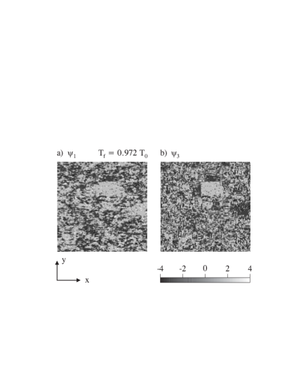
Let us start our description with thermally activated growth of the ordered phase, i. e. with the case of a shallow quench, $T_{0}>T_{f}>T_{sp}$. We then expect that the ordered regions – nuclei of the new phase – are repeatedly formed and destroyed by thermal fluctuations unless a nucleus exceeding a certain critical size is built. Once formed, such an overcritical nucleus will grow relatively fast against the surrounding disordered bulk until it meets another (growing) ordered domain. An $xy$–section of a configuration with overcritical nuclei formed in a system of $128\times 128\times 128$ fcc–cells is shown in Figs. 2a and 2b. It emerged 7000 MCS after the quench to $T_{f}=0.972\,T_{0}>T_{sp}$. The central nucleus seen in the figure is in fact composed of three “twinned” crystallites, corresponding to $\psi_{1}\simeq 2$ (the large, nearly homogeneous, bright spot in Fig. 2a) and $\psi_{1}\simeq-2$ (the neighboring dark spot). As shown in Fig. 2b, the homogeneous bright spot of Fig. 2a is in fact composed of two crystallites corresponding to $\psi_{3}\simeq-2$ and $\psi_{3}\simeq 2$, respectively. A second nucleus characterized by $\psi_{1}\simeq 2$ and $\psi_{3}\simeq-2$ grows at the right edge of the system. The configuration displayed in Figure 2 is quite typical for a quench temperature slightly above $T_{sp}$.

Figure 2: Thermally activated ordering in a system of $128\times 128\times 128$ fcc–cells at $T_{f}=0.972\,T_{0}>T_{sp}$. (a) $\psi_{1}$ and (b) $\psi_{3}$ patterns containing overcritical nuclei at a time $t=7\times 10^{3}$ MCS after the quench from random initial conditions (grey scales indicate local values of $\psi_{\alpha}$ ($\alpha={1,3}$) between $-4$ and $4$). (c) Histograms of corresponding $\Phi=(|\psi_{1}|+|\psi_{2}|+|\psi_{3}|)/3$ values averaged over blocs of $4\times 4\times 4$ fcc–cells calculated at a series of times after the quench.

To follow the ordering process that takes place in the whole volume of the system we now introduce an additional quantity Fron $\Phi=(|\psi_{1}|+|\psi_{2}|+|\psi_{3}|)/3$ as a convenient indicator of the degree of local order: $\Phi\simeq 0$ in the disordered phase and $\Phi\leq 2$ for any of the four equivalent ordered states. Further, we divide the system into blocs of $4\times 4\times 4$ fcc-cells, calculate $\Phi$ independently for each bloc to obtain a distribution function $P(\Phi,t)$ for a series of time intervals after the quench. For a quench to $T_{f}=0.972\,T_{0}$ the obtained histograms are shown in Fig. 2c. In this figure we easily identify three stages of the ordering process. First, up to several thousand MCS, the whole system remains disordered. The distribution of $\Phi$ broadens with time but stays concentrated close to $\Phi=0$. Then, after some incubation time, $\tau_{inc}$, see section IV, the second maximum close to $\Phi=2$ shows up. At that moment first overcritical nuclei emerge in the system and start to grow. The second stage, in which overcritical nuclei grow against the disordered bulk, is realized by histograms for $7\cdot 10^{3}\leq t\leq 10^{4}$ MCS in which both peaks are clearly visible. In the third stage, practically the whole system is already ordered and, as illustrated by curves for $t=2\cdot 10^{4}$ and $5\cdot 10^{4}$ MCS, the distribution of $\Phi$ changes very little with time. At that stage coarsening processes take place.

Figure 3: Continuous ordering in a system of $128\times 128\times 128$ fcc–cells at $T_{f}=0.5465\,T_{0}<T_{sp}$. (a) $\psi_{1}$ and (b) $\psi_{3}$ patterns at a time $t=7\times 10^{3}$ MCS after the quench from random initial conditions. Two types of domain walls are clearly shown. (c) Histograms of corresponding $\Phi$ values calculated at a series of times after the quench.

In contrast to the above sequence of events, deep quenches ($T_{f}<T_{sp}$) result in continuous ordering, in which shortly after the quench the whole volume of the system decomposes into ordered domains. As a representative example Figs. 3a and 3b display distributions of $\psi_{1}$ and $\psi_{3}$, respectively, for an $xy$–section through the system at $t=7\cdot 10^{3}$ MCS after a quench to $T_{f}=0.5465\,T_{0}$. The two types of domain walls, that may be formed in the system,KikuchiC ; Lai show up in Figs. 3a and 3b. The low–energy interfaces appear there as straight lines parallel to the $x$ or $y$–axis. Across each of these lines $\psi_{1}$ and $\psi_{3}$, or $\psi_{2}$ and $\psi_{3}$ simultaneously change sign across line–intervals parallel, to the $x$ or $y$–axes, respectively. Within the simple model used in this paper, formation of such walls costs no energy and therefore they are very stable. The curved interfaces seen in Fig. 3a consist of sectors of high–energy domain walls across which $\psi_{1}$ and $\psi_{2}$ change sign simultaneously. The histograms of $\Phi$–values obtained after averaging over 10 independent runs for $T_{f}=0.5465\,T_{0}$ are shown in Fig. 3c for a sequence of time intervals after the quench. There, in contrast to Fig. 2c, the initial peak at $\Phi=0$ spreads out within the first 100 MCS and the maximum at $\Phi\simeq 2$ starts to grow by 200 MCS to reach a considerable height already at $2\cdot 10^{3}$  MCS. The $\Phi\simeq 2$ peak is very narrow, indicating a nearly perfect local order in the system. Additional small, sharp peaks at multiples of $\Phi=0.5$ may be traced back to the domain walls that cross some of the blocs of $4\times 4\times 4$ fcc–cells used to prepare Fig. 3c. Slow coarsening processes, which in this case set in already for $t>2\cdot 10^{3}$ MCS result in considerable sharpening of the main $\Phi\simeq 2$ peak.

Figure 4: Volume fraction, $V_{ord}$, of an ordered phase ($\Phi>1.5$) as a function of time after the quench for a series of temperatures $T_{f}$.

To better illustrate the differences between the two ordering scenarios described above we show in Fig. 4 how $V_{ord}$, the volume fraction of the ordered phase, grows with time for a number of final temperatures. There, we counted as ordered all the blocs (of $4\times 4\times 4$ fcc–cells each) for which $\Phi>1.5$. The character of $V_{ord}(t)$ changes from a slowly increasing function of $t$ for $T_{f}\leq 0.911\,T_{0}$ to a sharp, nearly stepwise growth after some incubation time for $T_{f}>0.972\,T_{0}$.

In the next two sections we analyze in more detail the incubation time and the long time coarsening processes.

IV Incubation time

In the preceding section we introduced the incubation time $\tau_{inc}$ as the characteristic time interval between the quench and the observed growth of ordered domains in the case of metastability, $T_{f}>T_{sp}$. Let us now look more precisely at the processes that take place in the system within the initial stages of ordering. One relevant quantity here is the excess energy, $\Delta E(t)=E(t)-E(\infty)$, defined as the difference between the actual energy of the system, $E(t)$, and the energy it would reach after complete equilibration, $E(\infty)$. This means that we identify $E(\infty)$ with the energy of a single ordered domain of the size of the whole system, equilibrated at $T_{f}$. In Figure 5a $\Delta E(t)$ per lattice site is shown for a number of final temperatures $T_{f}$. Initially, the relaxation of $\Delta E(t)$ depends on temperature only weakly. Then, after about 20 MCS, the curves in Fig. 5a split due to a considerable slowing down of the relaxation rate with growing temperature. In turn, for shallow quenches, ordering proceeds in three stages, as displayed already in Fig. 2c. First, the system remains disordered up to a certain incubation time $\tau_{inc}$. The metastability of the ordered phase is reflected by plateaus in $\Delta E(t)$, which develop near $T_{f}\simeq T_{sp}$, and extend with increasing $T_{f}$. Second, $\Delta E(t)$ drops markedly when overcritical nuclei are produced by thermal fluctuations. We define $\tau_{inc}(T)$ as precisely that moment after the quench at which, for a given temperature $T$, $\Delta E(t)$ drops notably (by about 10 percent) below its plateau–value. The ordered nuclei formed within the incubation time grow against the disordered bulk until, in a third stage, ordered regions meet and slow coarsening processes set in.

In addition to $\Delta E(t)$, we also show in Figure 5b and 5c how the corresponding first moments of the structure factors $S_{\alpha}(k_{x},k_{y},k_{z},t)$ change with time. To account for the anisotropy illustrated in the domain patterns in Fig. 3a and b, we consider the two kinds of structure factors

$$S_{\parallel}(k,t)=\frac{1}{3}(S_{1}(k,0,0,t)+S_{2}(0,k,0,t)+S_{3}(0,0,k,t)),$$ (4)

and

$$S_{\perp}(k,t) = \frac{1}{N_{k}}\sum\limits_{q_{1}^{2}+q_{2}^{2}=k^{2}}(S_{1}(0,q_{1},q_{2},t)$$ (5)

$$+S_{2}(q_{1},0,q_{2},t)+S_{3}(q_{1},q_{2},0,t)),$$

where $N_{k}$ denotes here the number of $(q_{1},q_{2})$ pairs that fulfill $q_{1}^{2}+q_{2}^{2}=k^{2}$, as well as their first moments

$$k_{\parallel}(t)=\frac{\sum_{k>0}kS_{\parallel}(k,t)}{\sum_{k>0}S_{\parallel}(k,t)},$$ (6)

$$k_{\perp}(t)=\frac{\sum_{k>0}kS_{\perp}(k,t)}{\sum_{k>0}S_{\perp}(k,t)}.$$ (7)

Figure 5: Excess energy per lattice site $\Delta E$ (a), and the first moments $k_{\parallel}(t)$ (b) and $k_{\perp}(t)$ (c) of the structure factors $S_{\parallel}(k,t)$ and $S_{\perp}(k,t)$ as functions of time after the quench, calculated for a series of final temperatures $T_{f}$.

In Eq. (6) $k$ denotes one wave–vector component, see Eq. (4), while in Eq. (7) $k$ is defined as in Eq. (5). Clearly, $S_{\parallel}(k,t)$ is determined by structural modulations due to high–energy walls, which are reflected, for example, by sign–changes of $\psi_{1}$ when going along the $x$–axis, see Fig. 2. The quantity $k_{\parallel}$ therefore characterizes the inverse distance between such walls in one symmetry direction. On the other hand, $S_{\perp}$ is sensitive to the two-dimensional network of low–energy walls, and $k_{\perp}$ gives the inverse distance between such walls, cf. Fig. 3.

Curves displayed in all three parts of Figure 5 are strikingly similar in form, confirming that relaxation processes are indeed dominated by ordered domains growing in size. Moreover, $\Delta E$, $k_{\parallel}$ and $k_{\perp}$, all start to drop below their plateau–values at the same moment after the quench. This fact corroborates our linking the plateaus in $\Delta E(t)$ to the temperature-dependent incubation time for the formation of overcritical ordered nuclei. In accord with the spatial patterns shown in Figs. 2a, 3a and 3b, where high–energy walls are much further apart from each other than the low-energy ones, $k_{\parallel}(t)$ is in most cases considerably smaller than $k_{\perp}(t)$ calculated at the same temperature.

There are two effects restricting the range of $\tau_{inc}(T_{f})$ accessible to simulations. First, the system size $L$ must be considerably larger than the size of overcritical nuclei which are formed at temperature $T_{f}$. Second, obtaining smooth curves in Fig. 5 requires a sufficiently large number of nucleation events within the maximum computation time $t_{max}$. Again, this becomes increasingly difficult to fulfill with growing $T_{f}$ because both $\tau_{inc}$ and the dispersion of nucleation times over the different samples strongly increase with $T_{f}$. Comparing our results up to $t_{max}=5\cdot 10^{4}$ for lattices of size L=96 and L=128 we find $T_{f}\simeq 0.973\,T_{0}$ to be roughly the highest temperature for which $\tau_{inc}$ can be determined in a reliable way.

Figure 6: Incubation times $\tau_{inc}$ versus reduced temperature $T_{f}$. The inset shows the same data (full symbols) after conversion to the physical time scale as described in the text, together with incubation times measured Noda in Cu₃Au (open symbols).

Results of our simulations for $\tau_{inc}(T)$, plotted in Fig. 6, are consistent with the expression

$$\ln\tau_{inc}\propto(T_{0}-T_{f})^{-2},$$ (8)

which is similar in form to the nucleation rates obtained within classical nucleation theory Zettlemoyer ; BindStauf and Monte Carlo simulations.BindStauf ; StaufferA Note that the data point with $T_{f}/T_{0}=0.911$ falls well below the spinodal, but in Fig. 2 there still exists a shoulder at that temperature as a remnant of the plateaus at higher temperatures.

Incubation times for Cu₃Au have been measured by Noda et al. Noda from the width $\Gamma\propto k_{\perp}(t)$ of the (110) X-ray diffraction peak. Close to $T_{0}$ the width as a function of time develops plateaus qualitatively similar to Fig. 5c. Their data, however, refer to $T_{f}/T_{0}>0.981$, whereas ours are for $T_{f}/T_{0}\lesssim 0.976$. Also one should note that experimentally the ratio $T_{sp}/T_{0}$ may be sample–dependent. Because of the sensitivity of $\tau_{inc}$ to temperature differences with respect to $T_{sp}$, this introduces considerable uncertainties in our comparison. Nevertheless it is interesting to present experiments and simulations in one plot, as done in the inset of Fig. 6. There the simulation data were linked to the physical time scale exactly in the manner described towards the end of section II. Both sets of data display a remarkable similarity with respect to the order of magnitude in time and their trend with temperature (and even seem to be a continuation of each other). We conclude that the connection between time scales for diffusion (see section II) and nucleation as implied by our algorithm roughly agrees with experiment.

V Coarsening regime and scaling

As pointed out in the preceding sections, the distances between high– and low–energy walls define two different length scales. Moreover, the high–energy walls that are much further apart from each other than the low–energy ones, are also less stable. As a consequence, we expect direction–dependent scaling laws to hold for the structure factors $S_{\alpha}(\vec{k},t)$. This is made explicit by considering the functions $S_{\parallel}$ and $S_{\perp}$ introduced in Eqs. 4 and 5. Due to their definitions we expect these structure factors to obey scaling laws for one–dimensional and two–dimensional systems, respectively. This is verified by our simulations at $T_{f}=0.5465\,T_{0}$, i. e. in the case of continuous ordering. As shown by the $1d$ and $2d$ scaling plots in Figs. 6a and 6b, the data taken for a number of times $t\geq 500$ MCS after the quench indeed collapse onto single master curves. Moreover, the decay of both quantities at large k appears to be consistent with Porod’s law in $d=1$ and $d=2$, respectively,Porod ; comF

$$k_{\parallel}(t)S_{\parallel}(k,t)\propto(k/k_{\parallel}(t))^{-2},$$ (9)

$$k_{\perp}^{2}(t)S_{\perp}(k,t)\propto(k/k_{\perp}(t))^{-3}.$$ (10)

We now ask whether the same scaling laws apply to the results for $T_{f}>T_{sp}$, i. e. to the case of thermally activated ordering. Figure 8 contains the corresponding plots of $S_{\parallel}(k,t)$, part (a), and $S_{\perp}(k,t)$, part (b), calculated for $T_{f}=0.972\,T_{0}$ at times $t>\tau_{inc}$. In both parts of the figure scaling regimes are observed which are consistent with Eqs. (9) and (10) in an intermediate range of $k$–values. Both $S_{\parallel}$ and $S_{\perp}$, however, develop tails at large $k$ which show significant deviations from scaling. These deviations can be traced back to irregular shapes of overcritical nuclei growing against the disordered bulk (cf. Fig. 2). Such highly structured grain boundaries eventually meet, leading to likewise structured domain walls when the regime of slow coarsening is reached. Small inclusions of disordered phase still remain trapped between boundaries of ordered grains for quite a long time after the onset of coarsening processes in the bulk of the crystal.

Closer inspection of our data near the onset of those tails reveals that indeed, with increasing time $t$, the validity of Porod’s law extends to larger $k$ in both parts of Figure 8. We may take this as indication that Porod’s law, defined by Eqs. (9) and (10), will dominate in the late stages of continuous as well as thermally activated ordering processes.

Figure 7: Scaled structure factors $k_{\parallel}S_{\parallel}(k,t)$ (a) and $k_{\perp}^{2}S_{\perp}(k,t)$ (b) calculated for $T_{f}=0.5465\,T_{0}<T_{sp}$; the slopes of the dashed straight lines represent a decay according to $(k/k_{\parallel})^{-2}$ (a), and $(k/k_{\perp})^{-3}$ (b).

The last point we like to address concerns the observed growth rates of the characteristic domain–size, $l(t)$. Since the transition considered here is described by a set of non–conserved order parameters $\psi_{1}$ through $\psi_{3}$, one might expect that ordered domains grow according to the Lifshitz–Allen–Cahn law $l(t)\propto t^{\nu}$ with $\nu=1/2$.Lifsh ; AllenC Experiments on Cu₃Au indeed were interpreted in terms of this conventional growth law.Shan ; Noda ; Konishi In this context, however, one should be aware of the fact that systems of the type considered may show effective growth exponents during relaxation different from the Lifshitz–Allen–Cahn law. In the case of a vacancy mechanism effective exponents $\nu>1/2$ in principle can arise in models based on a non–conserved order parameter. In these studies,Vives ; Fratzl an increased $\nu$ was ascribed to an accumulation of vacancies within the domain boundaries, leading to an enhancement of the interfacial dynamics. For the present model we have verified, however, that the interaction parameters chosen do not favor segregation of vacancies in the domain boundaries.Porta Another modification of the Lifshitz–Allen–Cahn law that can act in the opposite direction results from local changes in composition within antiphase boundaries so that the ordering process gets coupled to a (slow) conserved order parameter component.

Figure 8: Same as in Fig. 7 but for $T_{f}=0.972\,T_{0}>T_{sp}$.

In our simulations we systematically observe effective growth exponents $\nu\simeq 1/4$ or even smaller (cf. Fig. 5 and Kessler et al. paper1 ). Moreover, within our accessible computing times ($3\cdot 10^{4}-~{}5\cdot 10^{4}$ MCS), these exponents depend slightly on temperature. One possible source of these differences between simulations and the experimental data ($\nu\simeq 1/2$) seems to be the existence of the low–energy type–I walls. Specifically, let us recall that our model contains only nearest neighbor interactions, so that type–I walls have zero energy and thus are extremely stable. It has been suggested previously that such a situation may lead to $\nu=1/4$.Castan ; Deymier Moreover, the present model does imply a coupling of the non–conserved order parameters to the conserved density $\psi_{0}$. This coupling becomes active within type–II walls. The relaxation of a modified composition within type–II walls is slowed down further because type–II walls are interconnected via type–I walls which have fixed $\psi_{0}$ and do not allow any exchange of composition. The slight upward bending of the low–temperature data in Fig. 5 at the longest times, indicating an even slower growth, might be interpreted in this way, although this point needs to be clarified in further studies.

VI Summary and conclusions

Implementing the vacancy mechanism in a model for the atomic dynamics in $A_{3}B$–type fcc–alloys, we investigated the growth of ordered domains after a temperature quench below the transition temperature $T_{0}$. Depending on the depth of the quench we observe two clearly distinct ordering–scenarios: thermally activated nucleation of the ordered phase for shallow quenches, $T_{0}>T_{f}>T_{sp}$, and spinodal ordering, when $T_{f}<T_{sp}$. Here, the spinodal temperature $T_{sp}$ was taken over from independent simulations at equilibrium.

In the case of thermally activated processes there is some characteristic incubation time, $\tau_{inc}$, after which a small fraction of the system is covered by overcritical nuclei. Detailed simulation results for $\tau_{inc}$, based on vacancy–atom exchange, were presented. The time period $t<\tau_{inc}$ manifests itself in plateau regions for energy relaxation and for the size of ordered domains, when plotted versus $t$. Clearly, $\tau_{inc}$ is expected to diverge as $T_{f}$ approaches $T_{0}$ from below. Within the simple model investigated here and the available maximum computing time, $\tau_{inc}$ grows more than 260 times in a narrow temperature interval above $T_{sp}$ – from about 90 MCS at $T_{f}=0.911\,T_{0}$ to roughly $24\cdot 10^{3}$MCS at $T_{f}=0.976\,T_{0}$. In comparison with measurements Noda of $\tau_{inc}$ this seems to constitute the correct order of magnitude when Monte Carlo times are converted to physical times with the help of experimental tracer diffusion coefficients. In the coarsening regime we observed growth of the characteristic domain–size that was clearly slower than the conventional $t^{1/2}$–law expected for curvature driven processes in the presence of non–conserved order parameters. This may be due to the enhanced stability of the low–energy domain walls in the case of nearest–neighbor effective interactions assumed in our model. The enhanced stability of low energy walls leads to strong anisotropies of the domain–shapes observed in our system, and furthermore, to independent scaling laws for the correlation functions $S_{\parallel}(k,t)$ and $S_{\perp}(k,t)$. These two functions scale according to Porod’s laws for dimensions one and two, respectively, when $T_{f}\ll T_{sp}$. For $T_{f}>T_{sp}$ strong deviations from these scaling laws are observed in the region of large $k$–values, due to highly structured domain walls which originate from the stage of fast growth of ordered nuclei against disordered bulk.

References

- (1) S. M. Allen and J. W. Cahn, Acta Metal. 24, 425 (1976).
- (2) Z.–W. Lai, Phys. Rev. B41, 9239 (1990).
- (3) C. Frontera, E. Vives, T. Castán, and A. Planes, Phys. Rev. B55, 212 (1997).
- (4) M. Kessler, W. Dieterich, and A. Majhofer, Phys. Rev. B64, 125412-1 (2001).
- (5) K. Binder and D. Stauffer, Adv. Phys. 25, 343 (1976) and references quoted therein.
- (6) M. Acharyya and D. Stauffer, Eur. Phys. J. B5, 571 (1998).
- (7) I. M. Lifshitz, Sov. Phys. JETP 15, 939 (1962); J. Exp. Theor. Phys. (U.S.S.R) 42, 1354 (1962).
- (8) S. M. Allen and J. W. Cahn, Acta Metall. 27, 1085 (1979).
- (9) K. Binder, Phys. Rev. Lett. 45, 811 (1980).
- (10) W. Schweika and D. P. Landau, Monte Carlo Studies of Surface–Induced Ordering in Cu3Au Type Alloy Models, Springer Proceedings in Physics, Vol. 83, Eds D. P. Landau, K. K. Mon, and H.–B. Schüttler, Springer–Verlag, Berlin, Heidelberg, 1998,pp 186–190.
- (11) B. E. Warren, X–Ray Diffraction, Addison–Wesley Publishing Company, Reading Massachusetts, 1969, pp 206–247.
- (12) R. Kikuchi and J. W. Cahn, Acta Metall. 27, 1337 (1979).
- (13) As a result, the ground state of that model in fact is infinitely degenerate.
- (14) M. Yamaguchi and Y. Shirai in Physical Metallurgy and Processing of Intermetallic Compounds, Eds N. S. Stoloff and V. K. Sikka, Chapman and Hall, New York, 1996. The data on vacancy formation in the disordered phase of Cu3Au reported in this paper lead to for the average vacancy concentration at .
- (15) T. Heumann, and T. Rottwinkel, J. Nucl. Mater. 69–70, 567 (1978).
- (16) S. Benci, G. Gasparrini, E. Germagnoli, and G. Schianchi, J. Phys. Chem. Solids 26, 687 (1965).
- (17) K. Binder, Rep. Progr. Phys. 50, 783 (1987) and references quoted therein.
- (18) A. M. Zettlemoyer, Nucleation, Dekker, New York, 1969.
- (19) Y. Noda, S. Nishihara, and Y. Yamada, J. Phys. Soc. Japan 53, 4241 (1984).
- (20) G. Porod, in Small Angle X–Ray Scattering, Eds O. Glatter and L. Kratky, Academic Press, New York, 1982.
- (21) In their simulations of the ordering kinetics in Cu3Au for Frontera et al.Fron noticed direction–dependent scaling and deviations of the structure factors from the 3-dimensional form of Porod’s law.
- (22) R. F. Shannon, Jr., S. E. Nagler, C. R. Harkless, and R. M. Nicklow Phys. Rev. B46, 40 (1992).
- (23) H. Konishi and Y. Noda, in Dynamics of Ordering Processes in Condensed Matter, Eds S. Komura and H. Furukawa, Plenum Press, New York, 1989, p.309.
- (24) E. Vives, and A. Planes, Phys. Rev. Lett. 68, 812 (1992).
- (25) P. Fratzl, and O. Penrose, Phys. Rev. B55, R6101 (1997).
- (26) M. Porta, E. Vives, and T. Castan, Phys. Rev. B60, 3920 (1999)
- (27) T. Castan, and P.-A. Lindgård, Phys. Rev. B43, 956 (1991).
- (28) P. A. Deymier, J. O. Vasseur, and L. Dobrzyński, Phys. Rev. B55, 205 (1997).