Experiments of Interfacial Roughening in Hele-Shaw Flows
with Weak Quenched Disorder

Abstract

We have studied the kinetic roughening of an oil–air interface in a forced imbibition experiment in a horizontal Hele–Shaw cell with quenched disorder. Different disorder configurations, characterized by their persistence length in the direction of growth, have been explored by varying the average interface velocity $v$ and the gap spacing $b$. Through the analysis of the rms width as a function of time, we have measured a growth exponent $\beta\simeq 0.5$ that is almost independent of the experimental parameters. The analysis of the roughness exponent $\alpha$ through the power spectrum have shown different behaviors at short ($\alpha_{1}$) and long ($\alpha_{2}$) length scales, separated by a crossover wavenumber $q_{c}$. The values of the measured roughness exponents depend on experimental parameters, but at large velocities we obtain $\alpha_{1}\simeq 1.3$ independently of the disorder configuration. The dependence of the crossover wavenumber with the experimental parameters has also been investigated, measuring $q_{c}\sim v^{0.47}$ for the shortest persistence length, in agreement with theoretical predictions.

I Introduction

The kinetic roughening of growing surfaces is a problem of fundamental interest in nonequilibrium statistical physics. The interest arises from theoretical, experimental, and numerical evidence of scale invariance and universality of the statistical fluctuations of rough interfaces in a large variety of systems Barabasi-Stanley ; Krug-Adv-Phys-97 ; Meakin-1998 . One candidate system is the roughening of a driven interface separating two fluids in a porous medium. This problem has important practical applications, and has time and length scales easily accessible in the laboratory. It allows different possible realizations, depending on the relative viscosities and wetting properties of the fluids involved wong-94 .

One of these possible realizations which has received considerable attention in recent years is imbibition, i.e. the situation in which a viscous wetting fluid (typically oil or water) displaces a second less–viscous, non–wetting fluid (typically air) which initially fills the porous medium. The motion of imbibition interfaces can be spontaneous, i.e. driven solely by capillary forces, or forced externally at either constant applied pressure or constant injection rate.

Although there have been many experimental investigations of the scaling properties of imbibition interfaces in the last years, some results, particularly the quantitative values of scaling exponents, remain controversial. The current situation for the case of spontaneous imbibition is reviewed in Ref. Dube-00 . The situation for the case of forced imbibition is summarized in Section II. The limitations of the experiments, in our opinion, arise firstly from the lack of precise knowledge of the properties of the disorder introduced by the model porous medium, and secondly from the related difficulty in tuning the relative strength of stabilizing to destabilizing forces in the flow. In the present work we have attempted to avoid these two limitations by using a particular model porous medium, consisting on a Hele–Shaw cell with precisely designed and controlled random variations in gap spacing.

In our setup, an initially planar interface becomes statistically rough on a mesoscopic scale, as a result of the interplay between (i) the stabilizing effects of the viscous pressure field in the fluid, and the surface tension in the plane of the cell, on long and short length scales respectively, and (ii) the destabilizing effect of local fluctuations in capillary pressure, arising from the random fluctuations in gap spacing, on short length scales. Although they have a different physical origin, the role of local fluctuations in capillary pressure, in our setup, is very similar to the role of wettability defects in the imperfect Hele–Shaw cell introduced by de Gennes deGennes , and studied by Paterson and coworkers Paterson .

In this paper we present a systematic experimental study of forced imbibition of our model porous medium, by a wetting silicone oil driven at constant flow rate. Since the competing forces in our system are the same as in a real porous medium, the physics governing roughening is very similar in the two cases. The relative importance of viscous forces can be finely tuned by changing the injection rate of the invading fluid, and the strength of capillary fluctuations can be tuned by adjusting the distance between the two glass plates. The sequence of photographs in Fig. 1 provides examples of the resulting interfaces.

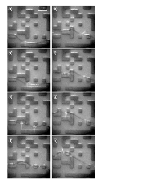
Figure 1: Eight consecutive close–up views of the oil–air interface advancing over the disorder. In each picture the oil is driven from bottom to top. The experimental parameters are gap spacing $b=0.36$ mm, average interface velocity $v=0.08$ mm/s, and disorder SQ 0.40. The time interval between images is 0.8 s.

The outline of the paper is as follows. Section II reviews the scaling properties of rough interfaces, and their experimental characterization in two–dimensional forced imbibition. Section III describes the experimental setup, Section IV introduces several parameters, such as permeability and modified capillary number, useful to characterize the experiments, and Section V explains the methodology used in data analysis. The experimental results are described in Section VI, and are analyzed and discussed in Section VII. The final conclusions are given in Section VIII.

II Scaling of rough interfaces

To be specific, let us consider a two–dimensional system with cartesian coordinates $(x,y)$, of lateral size $L$ in the $x$ direction and of infinite extension in the $y$ direction. The interface is driven in the direction of positive $y$, and its position at time $t$ is parametrized by the function $y=h(x,t)$. We assume that the interface is initially planar, $h(x,0)=0$. Let $w(l,t)$ (the rms interfacial width) denote the typical amplitude of transverse excursions on a scale $l$, parallel to the interface, at time $t$. For the complete interface:

$$w(L,t)=\left[\langle(h(x,t)-\widetilde{h}(t))^{2}\rangle_{x}\right]^{1/2},$$ (1)

where $\widetilde{h}(t)=\langle h(x,t)\rangle_{x}$. The notation $\langle\ldots\rangle_{x}$ represents an spatial average in the interval $[0,L]$, where $L$ is the system size. The standard picture of kinetic roughening is summarized in the dynamical scaling assumption of Family and Vicsek Family-Vicsek-1985 :

$$w(L,t)=L^{\alpha}\,g\left(t/L^{z}\right),$$ (2)

where $\alpha$ is the roughening (or static) exponent and $z$ is the dynamic exponent. The scaling function $g$ is:

$$g(u)\sim\left\{\begin{array}[]{l}u^{\alpha/z}\qquad\mbox{for}\qquad t\ll L^{z},\\ \mbox{constant}\qquad\mbox{for}\qquad t\gg L^{z}.\end{array}\right.$$ (3)

This picture assumes that the lateral correlation length of the interface fluctuations increases in time as $t^{1/z}$, in the $x$ direction. For all length scales $l$ within this correlation length the interface is rough, $w(l)\sim l^{\alpha}$. As the lateral correlation length increases, the interfacial width increases correspondingly with time as $w\sim t^{\alpha/z}$, which defines a growth exponent $\beta=\alpha/z$. Finally, when the lateral correlation length exceeds the system size, $L$, at a crossover time $t_{\times}\sim L^{z}$, the interface fluctuations saturate.

One way of measuring $\alpha$ is through the analysis of the interfacial width as a function of different system sizes $L$, i.e. $w(L)\sim L^{\alpha}$, at saturation. From an experimental point of view, however, it is not practical to perform experiments at different $L$. Usually it is prefered to measure $\alpha$ by analyzing $w$ for different window sizes $l$, with $l\leqslant L$. The scaling of $w(l)$ gives a local roughness exponent $\alpha_{loc}$, which is usually identified with the global exponent $\alpha$. This kind of analysis must be performed with some caution, however, because it can only provide $\alpha_{loc}\leqslant 1$ and hence fails for super–rough interfaces ($\alpha>1$). Moreover, a number of problems of kinetic roughening present intrinsic anomalous scaling, characterized by different values of local and global exponents Lopez-96-97 ; Ramasco-00 .

These difficulties can be overcome by analyzing the power spectrum of the interfacial fluctuations, defined as

$$S(q,t)=\langle H(q,t)H(-q,t)\rangle,$$ (4)

where

$$H(q,t)=\sum_{x}\left[h(x,t)-\widetilde{h}(t)\right]e^{iqx}.$$ (5)

The notation $\langle\ldots\rangle$ indicates average over disorder configurations. The mean width $w$ is related to $S(q,t)$ through

$$w^{2}(L,t)=\left(\frac{\Delta}{L}\right)^{2}\sum_{q}S(q,t),$$ (6)

where $\Delta$ is the sampling interval in the $x$ direction. For a 2–$d$ system, the equivalent of the Family–Vicsek scaling assumption for the power spectrum reads Lopez-96-97 :

$$S(q,t)=q^{-(2\alpha+1)}\,s\left(q\,t^{1/z}\right),$$ (7)

where the scaling function is given by

$$s(u)\sim\left\{\begin{array}[]{l}u^{2\alpha+1}\qquad\mbox{for}\qquad u\ll 1,\\ \mbox{constant}\qquad\mbox{for}\qquad u\gg 1.\end{array}\right.$$ (8)

The power spectrum can give values $\alpha>1$ and hence is applicable to super–rough interfaces. On the other hand, the presence of intrinsic anomalous scaling can be detected by a systematic shift of the power spectra computed at successive time intervals Lopez-96-97 .

The scaling concept has allowed a classification of kinetic roughening problems in universality classes characterized by different families of scaling exponents. The first class is described by the thermal Kardar–Parisi–Zhang (KPZ) equation KPZ-86 , which provides a local description of interfacial roughening in the presence of an additive white noise. The KPZ scaling exponents are $\beta=1/3$ and $\alpha=1/2$ in two dimensions. If the nonlinear term of the KPZ equation is supressed, the resulting equation is known as the thermal Edwards–Wilkinson (EW) equation EW-82 , which gives $\beta=1/4$ and $\alpha=1/2$ in two dimensions. When, instead of being purely thermal, the noise in the KPZ equation is supposed to depend on the interface height $h$, the equation displays a depinning transition. At the pinning threshold the interface behaviour of the complete equation with the nonlinear term (“quenched KPZ”) can be mapped to the directed percolation depinning (DPD) model, whose scaling exponents in two dimensions are $\beta=\alpha\simeq 0.633$. Suppressing the nonlinearity yields the “quenched EW” equation, for which $\beta\simeq 0.88$ and $\alpha\simeq 1$ in two dimensions Leschhorn-96-97 .

In the case of imbibition, there are two important issues which make the above classification of limited applicability. The first one is the quenched nature of the disorder. It has been argued that for very large driving the disorder may still be considered as a fluctuating in time (thermal) noise, but in general the disorder must be treated as a static, quenched noise. The second issue is the nonlocal character of the dynamics, due to fluid transport in the cell krug-91 ; he-92 . This issue has received important attention recently, with the introduction of imbibition models which take fluid transport explicitly into account, giving rise to nonlocal interfacial equations ganesan-98 ; Dube-teoric-99 ; Dube-teoric-00 ; Aurora-EPL-01 .

The models presented in ganesan-98 ; Dube-teoric-99 ; Dube-teoric-00 ; Aurora-EPL-01 are consistent with the well known macroscopic equations of the problem (Darcy’s law and interfacial boundary conditions). They differ in the way the noise is included in the equations and in the noise properties. The starting point of Ganesan and Brenner ganesan-98 is a random field Ising model. The permeability is taken spatially uniform and the noise exhibits long range spatial correlations. In the case of forced imbibition, and based on a Flory–type scaling, the model predicts that the roughness exponent $\alpha$ depends on the capillary number Ca, with asymptotic values $\alpha=3/4$ for the smallest drivings and $\alpha=1/2$ for the largest drivings. The approaches of Dubé et al. Dube-teoric-99 ; Dube-teoric-00 and Hernández–Machado et al. Aurora-EPL-01 are both based in a conserved Ginzburg-Landau model, where the noise is introduced in a fluctuating chemical potential or in the mobility, respectively, without long range correlations. Dubé et al. Dube-teoric-99 ; Dube-teoric-00 , however, consider only the case of spontaneous imbibition, which could give results very different from the case of forced imbibition, specially for the growth exponent $\beta$. By numerical integration they obtain $\alpha=1.25$ and $\beta=0.3$. Hernández–Machado et al. Aurora-EPL-01 study the case of forced imbibition, and predict a different scaling of the short and long length scales, with exponents $\beta_{1}=5/6,\alpha_{1}=5/2$ in the former regime, and $\beta_{2}=1/2,\alpha_{2}=1/2$ in the latter.

A common feature of these models, pointed out in Refs. Dube-teoric-99 ; Dube-teoric-00 ; Aurora-EPL-01 , is the presence of a new lateral length scale, $\xi_{c}$, related to the interplay of interfacial tension and liquid conservation. For $q\gg 1/\xi_{c}$ the dominant stabilizing contribution is the interfacial tension in the plane of the cell, while for $q\ll 1/\xi_{c}$ it is the fluid flow. The interplay leads to a dependence of $q_{c}$ ($=1/\xi_{c}$) on $v$ of the form $q_{c}\sim v^{1/2}$.

As mentioned in the introduction, the experimental characterization of the scaling properties of interfaces in two–dimensional forced imbibition remains conflicting. Most experiments have been conducted in model porous media consisting of air–filled Hele–Shaw cells packed with glass beads. In a first experiment of this sort on water–air interfaces, carried out by Rubio et al. Rubio-89 , a roughening exponent $\alpha=0.73\pm 0.03$ was measured, independent of Ca and bead size, for Ca values in the range $10^{-3}$ – $10^{-2}$. A controversial reanalysis of their data by Horváth et al. gave $\alpha=0.91\pm 0.08$ Horvath-90 ; Rubio-90 , which these authors compared to $\alpha=0.88\pm 0.08$ obtained in their own replication of the experiment. In a subsequent work Horvath-91 , using glycerol instead of water, Horváth et al. reported a clear power law growth regime with a growth exponent $\beta\simeq 0.65$, and different values $\alpha\simeq 0.81$ and $\alpha\simeq 0.49$ at short and long wavenumbers, respectively, at saturation. The last set of experiments of this kind is due to He et al. he-92 , who explored a very large range of Ca (from $10^{-5}$ to $10^{-2}$) and found large fluctuations of the roughness exponent in the saturation regime, between $0.65$ and $0.91$. In these experiments $w$ was shown to fluctuate wildly during growth, and it was impossible to give a value of the growth exponent $\beta$.

Other experiments have been directed to characterize the statistical properties of the avalanches displayed by imbibition fronts at sufficiently small Ca. The results are also conflicting. The first study Horvath-avalanches-91 was done on the same air-glycerol interfaces of Ref. Horvath-91 , and gave a power law distribution of avalanche sizes. The second one Dougherty-Carle-98 , on air–water interfaces, reported an exponential distribution.

In our experiments, the possibility of tuning the different competing forces has allowed an accurate measurement of the growth exponent $\beta$, by enlarging the growth regime before saturation. Fine tuning of the forces has also allowed to measure the crossover length $\xi_{c}$, and its dependence on velocity $v$.

III Experimental Setup

In our experiments a silicone oil (Rhodorsil 47 V) displaces air in a horizontal Hele-Shaw cell, $190\times 550$ mm², made of two glass plates 20 mm thick. The oil has kinematic viscosity $\nu=50$ mm²/s, density $\rho=998$ kg/m³, and surface tension oil–air $\sigma=20.7$ mN/m at room temperature. Fluctuations in the gap thickness are provided by a fiber-glass substrate, fixed on the bottom glass plate, containing a large number of copper islands which randomly occupy the sites of a square grid. The height of the islands is $d=0.06\pm 0.01$ mm. The gap spacing $b$, defined as the separation between the substrate and the top plate, is set by placing several calibrated spacers on the perimeter of the substrate, over the disorder, as shown in Fig. 2. We have used gap thicknesses in the range $b=0.16-0.75$ ($\pm 0.05$) mm.

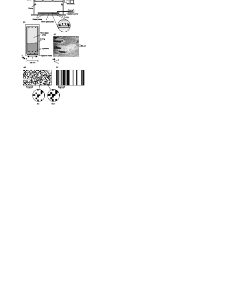
Figure 2: Sketch of the experimental setup. a) Side view. b) Top view. c) SEM image of the copper islands on the fiber–glass plate. d) and e) Partial views of the disorder pattern for d) squares (SQ, SQ-n) and e) tracks (T). The copper islands are the black regions. The blow–ups in d) show the detailed structure of the disorder pattern for SQ and SQ-n.

The disorder pattern is designed by computer and manufactured using printed circuit technology. In order to clearly identify the oil–air interface when it moves over the copper islands, the plates have been chemically treated to accelerate copper oxidation. Otherwise the copper islands are too bright to recognize the interface contour. The silicone oil wets perfectly both fiber–glass and copper, and no differences in the wetting properties due to the oxidation protocol have been observed.

For each experiment, the glass plates are cleaned with soap and water and rinsed with distilled water and acetone. The fiber–glass plate is cleaned using blotting–paper only, which leaves a thin layer of oil to avoid further oxidation of the copper surface, ensures a complete wetting in both fiber–glass and copper, and improves the interface contrast in the captured images. Next, the fiber–glass plate is fixed over the bottom glass plate using a thin layer of removable glue. The cell is completed by placing the spacers, the upper glass plate, and the o–ring around the fiber–glass plate (Fig. 2). Finally, the two glass plates are firmly clamped together, to ensure the homogeneity of the gap spacing and the tightness of cell sides closed by the o–ring.

The oil is injected at constant flow-rate using a syringe pump Perfusor ED-2. The syringe pump can be programmed to give flow–rates $Q$ in the range 1–299 ml/h with less than 2 % fluctuations around the nominal value. The oil enters the cell through two wide holes, drilled on the top plate near one end of the cell. The other end of the cell is left open. To start the experiment with as flat an interface as possible, the oil is first slowly injected on a transverse copper track, on the fiber-glass plate, which is 2 mm ahead the disorder pattern. Next, the syringe pump is set to its maximum injection rate until the whole interface has reached the disorder (about 3 s later). The pump is then set to the nominal injection rate of the experiment, and $t=0$ is defined as the time at which the average height of the interface (measured on the images) reaches the preset nominal velocity.

The oil–air interface evolution is monitored using two JAI CV-M10BX progressive scan CCD cameras (each camera acquiring half side of the cell). The 1/2” CCD sensor contains 782 (H) $\times$ 582 (V) pixels. In our experiment we have used an exposure time of 1/25 s in order to minimize the illumination. Each camera is equipped with a motorized zoom lens Computar M10Z1118MP with a focal length in the range 11–110 mm (1:10 zoom ratio). The cameras are connected to an Imaging Technology PCVision frame grabber installed in a personal computer. A Visual Basic application controls both cameras and stores the images for further analysis.

The images are taken with a spatial resolution of 0.37 mm per pixel, a size of $768\times 574$ pixels, and 256 grey scale levels per pixel. The acquisition is logarithmic in time, with temporal increments that vary from 0.33 s to 180 s. Between 100 and 300 images are taken per experiment. Because the background is the same for all the images captured with the same camera, the interface is enhanced by subtracting the first image to all other images, and thresholding the result to get a black and white contour of the interface. The contour is resolved with 1–pixel accuracy using edge detection methods, and data are stored for further analysis. This method is automatically performed, with an error in the interface recognition comparable to the width of the oil–air meniscus, about one half the gap width. Fig. 3 presents two examples of the digitized interfaces, compared with the original images.

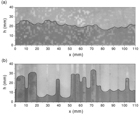
Figure 3: Interface profiles for two types of disorder configurations, SQ 1.50 (a) and T 1.50 (b), compared with the original digital images. The copper islands are the brighter spots of the image background. The experimental parameters are $b=0.36$ mm and $v=0.08$ mm/s in the two cases.

IV Characterization of the experiments

IV.1 Disorder properties

Three kinds of disorder patterns have been used. Two of them are obtained by random selection of the sites of a square lattice (Fig. 2(d)). In the first of them (SQ) we allow nearest neighbour connections only, leaving next–nearest neighbours separated by 0.08 mm. In the second one (SQ-n) both nearest neighbour and next–nearest neighbour connections are allowed. The third kind of disorder pattern (T) is formed by parallel tracks, continuous in the $y$ direction and randomly distributed along $x$ (Fig. 2(e)). The filling fraction $f$ (fraction of lattice sites occupied by copper) is 35 % in the three cases. However, $\widetilde{l}$, the persistence length of the disorder in the direction of growth, is very different in the three different disorder patterns. This length is measured in the following way: (i) We consider every site $x$ of the lattice along the lateral direction, and measure the average length $l(x)$ of the island formed by the connected copper sites at $x-\Delta x$, $x$, and $x+\Delta x$, where $\Delta x$ is the lattice spacing. (ii) We average $l(x)$ over the lateral direction in the interval $(0,L)$. As can be seen in the inset of Fig. 4, $\widetilde{l}$ increases by a factor $2.4$ when changing from SQ to SQ-n, and up to the total length of the cell for T. Another characteristic of the disorder is the cluster size, which gives the number of disorder unit cells of the copper aggregations. The statistical distribution of copper clusters is shown in the main plot of Fig. 4.

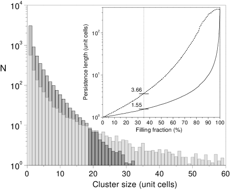
Figure 4: Statistical distribution of the copper clusters for a filling fraction $f=0.35$. Clusters with only nearest neighbour contacts (SQ) are represented in dark grey. Clusters with nearest and next–nearest neighbour contacts (SQ-n) are represented in light grey. The inset shows the persistence length of the disorder $\widetilde{l}$ as a function of the filling fraction $f$. The solid and dashed lines correspond to the SQ and SQ-n cases respectively. The vertical line indicates the filling fraction used in our experiments.

We have used two values of the lattice spacing in the lateral direction, $\Delta x=1.50\pm 0.04$ mm and $0.40\pm 0.04$ mm. From here on we refer to the disorder used in a given experiment by SQ, SQ-n, or T, followed by the lateral size in mm of the disorder unit cell, $1.50$ or $0.40$.

IV.2 Permeability

To characterize the fluid flow through our Hele–Shaw cell with disorder, we have determined the permeability of the cell for the different disorder patterns as a function of the gap spacing. The experimental set up used for this purpose is similar to the one shown in Fig. 2, but the injection system has been replaced by a constant pressure device. It consists of an oil column of adjustable constant height in the range from 200 $\pm$ 2 mm to 1000 $\pm$ 5 mm. The permeability is determined by measuring the oil–air interface average velocity for different applied pressures (heights of the oil column) and using Darcy’s law,

$$\vec{v}=-\frac{k}{\mu}{\vec{\nabla}}p,$$ (9)

where $\vec{v}$ is the interface velocity, $k$ the permeability, $\mu$ the dynamic viscosity, and ${\vec{\nabla}}p$ the pressure gradient.

Fig. 5 shows the results obtained. At large gap spacings, $d/b\rightarrow 0$, the disorder has no effect on the fluid flow, and the permeability tends to the expected value for an ordinary Hele–Shaw cell, $k_{0}=b^{2}/12$, independently of the disorder configuration. At very small gaps, $d/b\rightarrow 1$, the permeability decreases, and tends to a non–zero value $k_{1}$ for $d/b=1$, that clearly depends on the disorder configuration. We have found it convenient to write $k_{1}$ in the form

$$k_{1}=d^{2}{\Lambda}/12,$$ (10)

where $\Lambda$ is a function that depends on the porosity $\phi$ and the geometry of the disorder. The simplest functional form that interpolates between these two limits can be written as:

$$k=\frac{b^{2}}{12}\left(1-(1-{\Lambda}^{1/2})\frac{d}{b}\right)^{2}.$$ (11)

The coefficient $\Lambda$ can be obtained in general from a fit of the permeability to the experimental data.

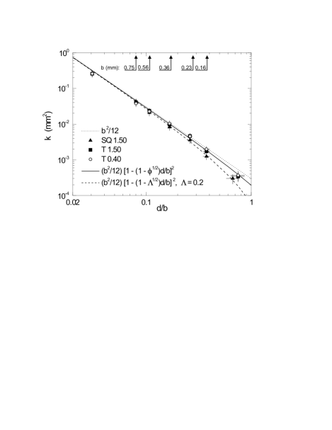
Figure 5: Measurements of the permeability, $k$, as a function of the disorder strength, $d/b$, for $d=0.06$ mm. The dotted line is the permeability of an standard Hele–Shaw cell (without disorder), and the dashed and solid lines are fits to the experimental data for SQ and T disorder configurations, respectively. The arrows point to the values of $d/b$ for the gap spacings used in the experiments.

In the particular case of disorder T and $d/b=1$, an analytic expression of $\Lambda$ can be derived by recognizing that the cell in this case is formed by a parallel array of rectangular capillaries. Following Avellaneda et al. Avellaneda91 , in this geometry $\Lambda$ is directly the porosity $\phi$, which in the limit $d/b=1$ is given simply by $\phi=1-f$. Hence, since we have $f=0.35$, we obtain $\Lambda=0.65$. This result fits well the experimental data not only in the limit $d/b=1$ but also in the whole range of $d/b$ (solid line in Fig. 5). Notice also that the results presented in Fig. 5 show that there are no important differences between T 1.50 mm and T 0.40 mm. This observation generalizes the theoretical result that in the limit $d/b=1$ the width of the rectangular capillaries does not modify the permeability Avellaneda91 . For SQ and SQ–n disorder, due to the difficulty of finding a general expression for $k_{1}$ (see Refs. Koponen96 ; Koponen97 ), we have fitted $k$ to our experimental results (dashed line in Fig. 5) and have obtained a numerical value $\Lambda=0.20$.

IV.3 Capillary pressure

Assuming local thermodynamic equilibrium, the capillary pressure jump at the interface is given by

$$p^{+}-p^{-}=\sigma(\kappa_{\parallel}+\kappa_{\perp}),$$ (12)

where $\kappa_{\parallel}$ and $\kappa_{\perp}$ are the main curvatures of the interface, in the plane of the cell and perpendicular to it, respectively.

$\kappa_{\parallel}$ varies from $0$ for $d/b\ll 1$, to $2/r$ for $d/b\simeq 1$, where $r\simeq 1.75$ mm is the average diameter of the copper obstacles. In the range of gap spacings explored we have measured curvatures in the range $3.3\times 10^{-3}\leqslant\kappa_{\parallel}\leqslant 1.15$ mm^-1. Notice that $\kappa_{\parallel}\ll\kappa_{\perp}$ in all the range of gap spacings used in the experiments.

In ordinary Hele–Shaw flows (without disorder) $\kappa_{\perp}$ is roughly the same in all points of the interface and therefore adds only a constant contribution to the pressure jump. In our case, however, when the interface is over the copper islands (gap thickness $b-d$) we have:

$$\kappa_{\perp}=\frac{2}{b}\left(\frac{1}{1-d/b}\right),$$ (13)

and when it is over the fiber–glass substrate (gap thickness $b$):

$$\kappa_{\perp}=\frac{2}{b},$$ (14)

assuming complete wetting.

This difference in curvature, given by

$$\Psi=\frac{2}{b}\left(\frac{d/b}{1-d/b}\right),$$ (15)

makes the interface experience a capillary instability when it passes from one gap spacing to the other. In the range of gap spacings studied, $0.16\leqslant b\leqslant 0.75$ mm, we get $7.5\geqslant\Psi\geqslant 0.23$ mm^-1. We have verified that for gap spacings $b\gtrsim 2$ mm, which correspond to $\Psi\lesssim 0.031$ mm^-1, the fluctuations in capillary pressure are no more sufficient to roughen the interface appreciably.

IV.4 Modified capillary number

Once the permeability of the cell has been characterized, we can introduce a dimensionless number to describe the relative strength of viscous to capillary forces. The simplest number that relates viscous and capillary forces is the capillary number Ca$=\mu v/\sigma$. In order to account for the properties of the disorder, which are not contained in the previous definition of Ca, it is customary to introduce a modified capillary number. For an ordinary Hele-Shaw cell (without disorder), the modified capillary number, which we call Ca^∗, comes out from the dimensionless form of the Hele–Shaw equations Homsy87 :

$$\mbox{Ca}^{*}=\mbox{Ca}\cdot 12\left(\frac{L}{b}\right)^{2}.$$ (16)

To define a modified capillary number Ca’ for our particular cell with disorder, we consider on one side the average viscous pressure drop across the cell, given by

$$\delta p_{vis}=L\cdot|\nabla p_{vis}|,$$ (17)

with $\nabla p_{vis}=-v\mu/k$ (Darcy’s law). $L$, the cell width, provides the macroscopic length scale. On the other side, a measure of the capillary pressure drop is given by

$$\delta p_{cap}=\sigma\left(\frac{2}{b-d}-\frac{2}{b}+\frac{1}{L}\right).$$ (18)

The last contribution accounts for the curvature of the interface in the plane of the cell, and is relevant only when $d/b\to 0$, i.e. when the destabilizing role of the disorder vanishes.

Defining Ca’ $=\delta p_{vis}/\delta p_{cap}$ and using (11), (17) and (18), we get

$$\mbox{Ca'}=\mbox{Ca}\cdot\frac{12L}{\displaystyle b^{2}\left(1-(1-{\Lambda}^{1/2})\frac{d}{b}\right)^{2}\left(\frac{2}{b-d}-\frac{2}{b}+\frac{1}{L}\right)}.$$ (19)

The ratio Ca’/Ca^∗ as a function of $d/b$ is shown in Fig. 6 for disorders SQ and T. When $d/b\to 0$ the destabilizing role of the disorder is negligible, as expected, and Ca’/Ca^∗ tends to $1$ (ordinary Hele-Shaw cell). As $d/b$ increases, the increasing strength of the disorder is manifest in the progressive decrease of Ca’/Ca^∗. It is important to notice that our definition of Ca’ is not valid for $d/b=1$, because the flow would be essentially different when the free gap disappears. In the range of $d/b$ explored in our experiments the permeability of the cell remains always close to that of an ordinary Hele–Shaw cell (Fig. 5), and the decrease of Ca’/Ca^∗ is essentially due to the capillary forces associated with the menisci in the $z$ direction.

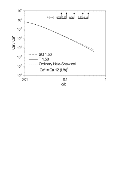
Figure 6: Ratio of the modified capillary number for the cell with disorder, Ca’, to the modified capillary number for an ordinary Hele-Shaw cell, Ca^∗, as a function of the disorder strength, $d/b$. The dashed and solid lines correspond to disorders SQ 1.50 and T 1.50. The dotted line represents the asymptotic limit Ca’$=$Ca^∗. The arrows point to the values of $d/b$ for the gap spacings used in the experiments.

In the range of gap spacings experimentally explored, $0.16\leqslant b\leqslant 0.75$ mm, the ratio between the free gap $b-d$ and the total gap $b$ varies between 62% and 92%. These large ratios, combined with the high viscosity and small surface tension of the silicone oil compared with other fluids (i.e. water), are responsible for the large values of Ca’ in our experiments, in comparison to the values reported for pure porous media. Considering for example the disorder T 1.50 mm, Ca’ varies from a value $1.33$ (for $b=0.16$ mm and the minimum interface velocity, $0.04$ mm/s) to a value $17.0$ (for $b=0.75$ mm and the maximum interface velocity, $0.4$ mm/s).

V Data Analysis

The wetting of the lateral gap spacers by the invading oil changes the physics at the two ends of the interface. To minimize this disturbance, which is particularly important at large gap spacings, we have disregarded 8 mm at each side of the cell, thereby reducing the measured interface from 190 to 174 mm in the $x$ direction. The final number of pixels of the interface after this correction is reduced from 515 to 470. For data analysis convenience these pixels are converted into $N=512$ equispaced points, through a linear interpolation. The final spacing between two consecutive points is $\Delta=L/N=0.34$ mm . Although the linear interpolation introduces an artificial resolution 7 % larger than the resolution of the original image, the increase does not affect the final analysis.

The interfaces measured at the smallest gap spacings and velocities may present overhangs. These multivaluations, rather exceptional, have been eliminated by taking for each value of $x$ the corresponding largest value of $h(x)$.

In addition, we have forced periodic boundary conditions for $h(x,t)$ by subtracting the straight line connecting the two ends of the interface. This procedure is well documented in the literature of kinetic roughening Simonsen98 . The linear correction imposed to the interfaces has significant effects on the power spectrum. The Fourier spectrum of an interface which is discontinuous at the two end points is dominated by an overall behaviour of the form $q^{-2}$. Forcing periodic boundary conditions eliminates the overall slope -2 Schmittbuhl95 . Moreover, the analysis of $w(l)$ is insensitive to the linear correction of the interface (except for values of $l$ comparable to the system size) and gives results consistent with those obtained from $S(q,t)$ only for interfaces with periodic boundary conditions.

Since the maximum width of the meniscus is only one half the gap width (in conditions of complete wetting) the interface can be considered one–dimensional at the length scale of the copper islands. The resolution of the interface fluctuations in the $y$ direction is $\pm$1 pixel at a given point. Nevertheless, the measurement of the global interfacial width $w$ is much more precise because the width is an average over the $N=512$ points of the interface.

Given that, according to our choice of the time origin, the whole interface is already inside the disorder at $t=0$, $w(0)\neq 0$. For this reason, we have decided to characterize the interface fluctuations by the subtracted width $W$, defined by $W^{2}(t)=w^{2}(t)-w^{2}(0)$ Barabasi-Stanley ; Tripathy00 . Notice that, since the data analysis is based on power law dependencies, short times are very sensitive to the definition of $t=0$ and to the value $w(0)$. After analyzing the data for different definitions of $t=0$, and checking the influence of subtracting $w(0)$, we have found that the analysis based on the subtracted width is the most objective and less sensitive to the details of the experimental procedure. The error bars shown in the $W(t)$ plots indicate the dispersion of the different individual experiments with respect to the average curve plus the uncertainty in the determination of $t=0$.

Finally, the crossover time $t_{\times}$ has been measured on the $W(t)$ log-log plots as the time when the power law with slope $\beta$ crosses the horizontal straight line that corresponds to the average value of the interfacial width at saturation, $W_{s}$.

VI Experimental results

The parameters explored in our experiments are summarized in Table 1. The minimum velocity selected in the experiments, $v=0.04$ mm/s (which will be taken as reference unit for interfacial velocities), has been chosen to ensure that the interface is always single–valued for gap spacings $b\gtrsim 0.36$ mm. We have used three different disorder realizations for SQ and SQ-n and four for T. For each disorder realization and each set of experimental parameters ($v$, $b$) we have carried out three runs for SQ and SQ-n, and two runs for T.

Disorder	Gap spacing (mm)	Interface velocity ($V=0.04$ mm/s)
SQ 1.50	$0.16,0.23,0.36,0.56,0.75$	$2V$
SQ 1.50	$0.36$	$V,2V,5V,7V,10\,V$
SQ-n 1.50	$0.36$	$V,2V,10\,V$
T 1.50	$0.16,0.36,0.56,0.75$	$2V$
T 1.50	$0.36$	$V,2V,5V,10\,V$
SQ 0.4	$0.36$	$2V$
T 0.4	$0.36$	$2V$

Table 1: Summary of the parameters explored for each kind of disorder.

VI.1 Variable velocity

VI.1.1 SQ 1.50 mm

We have started the study exploring five different velocities, from $V$ to $10\,V$, using an intermediate gap spacing $b=0.36$ mm. We have not selected velocities lower than $V$ to avoid overhangs and trapped air. An example of the interfaces obtained at different velocities is presented in Fig. 7. All the experiments shown correspond to the same disorder configuration, and the average position of the selected interfaces is also the same for the different velocities. The most noticeable aspect of the sequence of interfaces is that the short length scales are not affected significantly by the velocity, as opposite to the long length scales, which become progressively smoother as the velocity increases.

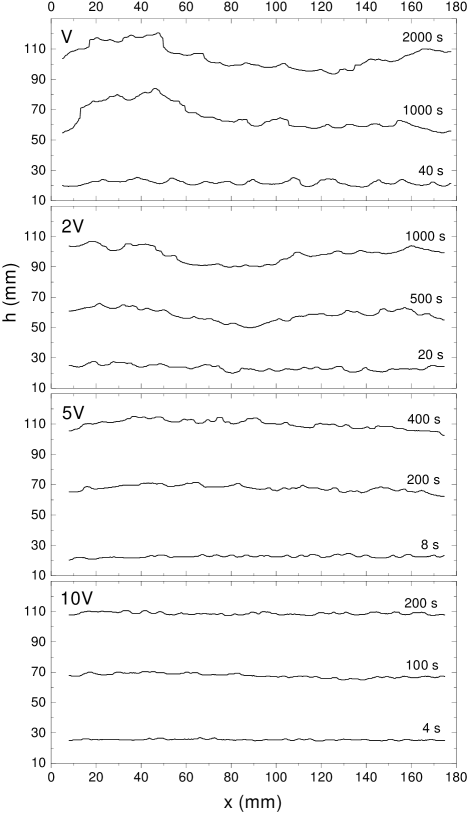
Figure 7: Sequence of interfaces at different velocities, for $b=0.36$ mm and disorder SQ 1.50, corresponding to Ca’$=1.85$, $3.69$, $9.24$, and $18.5$. The disorder realization is the same in the four sequences. The reference velocity is $V=0.04$ mm/s.

Fig. 8 shows the $W(t)$ plot for four different velocities. We have omitted the curve for $7V$ because it is too close to the $10\,V$ curve. All curves display a power law growth regime with approximately the same growth exponent $\beta=0.47\pm 0.04$, independent of the velocity. Saturation times and saturation widths depend clearly on the velocity, both decreasing at increasing velocities. This general behaviour is not so clear for the two smallest velocities, for which the corresponding $t_{\times}$ and $W_{s}$ are practically the same. This can be a consequence of the fact that the interface at very low velocity gets locally pinned at the end of the copper obstacles, hindering an arbitrary deformation of the interface. The strong fluctuations of $W$ that can be observed both during growth and at saturation are also remarkable. These fluctuations have two origins: the intrinsic metastabilities in systems with quenched–in disorder he-92 , and to a lesser degree the inhomogeneities in the gap thickness caused by small deformations in the fiber-glass substrate or small differences in the height of the copper obstacles. To smooth out the fluctuations it would have been necessary to increase the number of disorder configurations and runs to a number that would be prohibitive. Nevertheless, the largest fluctuations usually appear deep in saturation and do not change the results presented here.

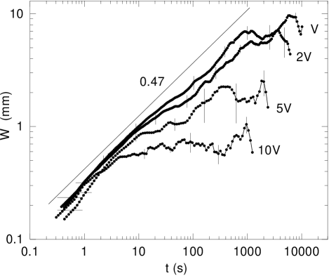
Figure 8: Interfacial width, $W(t)$, for disorder SQ 1.50, gap spacing $b=0.36$ mm, and four different velocities. The straight line drawn to guide the eye is the power law $W\sim t^{0.47}$.

Fig. 9 shows the analysis of the interface fluctuations through the power spectrum. An example of the temporal evolution of the spectrum, which corresponds to the experiments at velocity $2V$, is presented in Fig. 9(a). Since larger length scales become progressively saturated with time, the spectrum at short times displays a power law decay for large $q$ only. As time increases the power law extends to smaller $q$ until a second power law behaviour emerges, which reaches the smallest $q$, corresponding to the system size $L$, at saturation. The first power law regime (large $q$) will be characterized with a roughness exponent $\alpha_{1}$, and the second one (small $q$) with a roughness exponent $\alpha_{2}$. In the range of parameters explored we have always observed $\alpha_{1}>\alpha_{2}$. It is interesting to notice that the first regime shows a slightly time–dependent behaviour. $\alpha_{1}$ is progressively smaller as time increases, and reaches a constant value at saturation. This temporal dependence disappears at either high interface velocities or large gap spacings.

The power spectrum at saturation for five different velocities is shown in Fig. 9(b). The different behaviour at short and long length scales is visible in all cases, but the crossover from one regime to another (characterized by the wavenumber $q_{c}$ at the crossing point of the two power laws) increases systematically with increasing velocities.

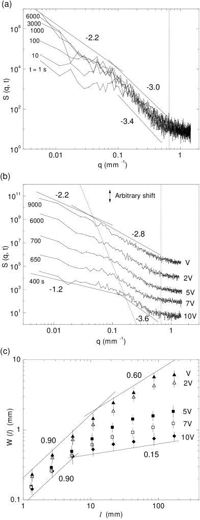
Figure 9: Determination of the roughness exponents for experiments at five different velocities, with $b=0.36$ mm and disorder SQ 1.50. a) Example of the temporal evolution of the power spectrum for velocity $2V$ (Ca’=$3.69$). b) Power spectra at saturation for the five velocities studied. The curves have been shifted in the vertical direction for clearness. c) Analysis of the local width, $W(l)$. The vertical lines in (a) and (b) give the value of $q$ associated with the spatial scale of the disorder. The tilted line crossing the power spectra in (b) fits the values of the crossover wavenumber $q_{c}$ at the different velocities. The other straight lines are power law fits from which the roughness exponents can be deduced.

The exponent $\alpha_{1}$ (large $q$) increases with the interface velocity, from a value $\alpha_{1}=0.9\pm 0.1$ (slope $=-2.8\pm 0.2$) at velocity $V$ to a value $\alpha_{1}=1.3\pm 0.1$ (slope $=-3.6\pm 0.2$) at velocity $10\,V$. We have observed that the variation is not linear, but tends to the limiting value $\alpha_{1}=1.3$ at large velocities.

The exponent $\alpha_{2}$ (small $q$) decreases with the interface velocity, varying from $\alpha_{2}=0.6\pm 0.1$ (slope $=-2.2\pm 0.2$) at velocity $V$ to $\alpha_{2}=0.1\pm 0.1$ (slope $=-1.2\pm 0.2$) at velocity $10\,V$. This exponent seems to be insensitive to the velocity at low velocities.

Fig. 9(c) shows the alternative analysis carried out to determine the roughness exponents, using $W(l)$. Notice that because this is a local analysis it is limited to a maximum value $\alpha=1$. At short length scales we obtain $\alpha_{1}=0.90\pm 0.1$ for all the velocities. The value $\alpha_{1}=1$ that we should have obtained for $v\geqslant 2V$ is unreachable because the fluctuations in $W(l)$ contribute always in the direction of decreasing $\alpha_{1}$. At long length scales the values obtained for $\alpha_{2}$ are consistent with the values measured from the power spectrum.

VI.1.2 Effect of increasing the persistence of the disorder

We have carried out a series of experiments oriented to explore how different kinds of disorder patterns affect the interfacial dynamics, and the possible universality of our results. The gap spacing and velocity used in all cases are $b=0.36$ mm and $2V$.

When the correlation length of the disorder in the $y$ direction is increased (changing the disorder pattern from SQ to SQ-n and then to T), we observe important differences in the behaviour of both $W(t)$ and $S(q,t)$. The correlation length of the disorder in the $y$ direction is quantified through the average extent of the disorder cells in the $y$ direction, $\widetilde{l}$, introduced in Sec. IV.1. For a basic disorder cell of size 1.50 mm, $\widetilde{l}\simeq 2$ mm for SQ, $\widetilde{l}\simeq 5$ mm for SQ-n, and $\widetilde{l}=\infty$ for T. The immediate consequence of a progressively larger correlation length is the persistence of the capillary forces for longer times. The effect on $W(t)$ is that the large fluctuations observed during growth disappear as $\widetilde{l}$ increases. In the extreme limit of disorder T, $W(t)$ is a neat power law with an exponent $\beta=0.52\pm 0.03$, as can be seen in Fig. 10(a). Other relevant aspects are that the saturation times can be clearly identified and the fluctuations in saturation have a minor amplitude. Whereas the important fluctuations of $W(t)$ both during growth and saturation, together with substantial differences between different runs and disorder configurations, are characteristic of the experiments with SQ, for T the experiments show that different runs with the same disorder configuration lead to practically identical results, and differ only slightly when the disorder configuration is changed.

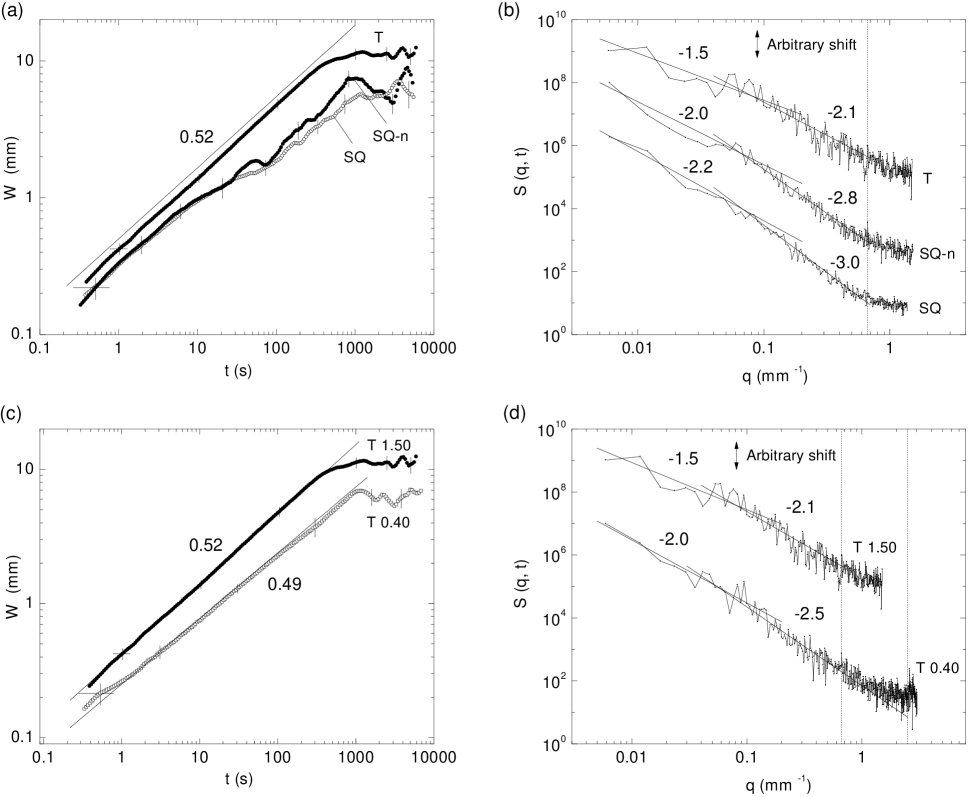
Figure 10: Interfacial width $W(t)$ (a) and power spectra $S(q,t)$ (b) for three kinds of disorder with unit cell of size 1.50 mm. c) and d) show the same magnitudes for disorder T of two different sizes, 0.40 and 1.50 mm. The spectra have been shifted in the vertical direction for clearness. The vertical lines give the value of $q$ associated with the spatial scale of the disorder. In all the experiments $b=0.36$ mm and $v=2V$ (Ca’$=3.25$ for T, and $3.69$ for SQ and SQ-n).

The increasing correlation length in the direction of growth has important consequences in the power spectrum. On one side, the observation of a smaller roughness exponent $\alpha_{1}$ as time increases for disorder SQ (Fig. 9(a)), is more evident as we go to SQ-n and T. The exponent $\alpha_{1}$ obtained for different disorders, however, tends to a single value at large gap spacings and high velocities (weak capillary forces). On the other side, the spectra at saturation shown in Fig. 10(b), clearly indicate that a progressively larger $\widetilde{l}$ reduces the measured roughness exponents, from $\alpha_{1}=1.0\pm 0.1$ to $\alpha_{1}=0.5\pm 0.1$, and from $\alpha_{2}=0.6\pm 0.1$ to $\alpha_{2}=0.2\pm 0.1$, as the disorder changes from SQ to T. This trend is confirmed by experiments using SQ 0.40 ($\widetilde{l}\simeq 0.6$), where the evolution of $\alpha_{1}$ with time is not observed due to the short $\widetilde{l}$ and, at saturation, gives exponents $\alpha_{1}\simeq 1.1$ and $\alpha_{2}\simeq 0.5$.

Another interesting modification that can be introduced in the disorder is the size of the basic disorder cell. In addition to our usual experiments with lateral size 1.50 mm, we have made experiments with disorder T of lateral size 0.40 mm. The $W(t)$ curves for both cases are shown in Fig. 10(c). Both curves give approximately the same growth exponent, around $\beta=0.50$. The small differences in slope around this value can be attributed to the reduced number of disorder configurations studied. The most noticeable difference is the saturation width, which is smaller for the small disorder size. The power spectrum at saturation for the two cases is shown in Fig. 10(d). Notice that in the case of T 0.40, the measured exponents $\alpha_{1}$ and $\alpha_{2}$ increase considerably, and approach the values measured for SQ or SQ-n 1.50.

VI.1.3 T 1.50 mm

Here we present a systematic study of the disorder T 1.50, in the same line as for SQ 1.50 (Sec. VI.1.1). The disorder T 1.50 ensures that the interface is always single–valued at any gap spacing and velocity, which allows exploring a wide range of experimental parameters.

Fig. 11 shows an example of the interfaces obtained in the experiments with T 1.50 at different velocities and fixed gap spacing. As we observed for SQ 1.50, the interfaces become progressively flatter as the velocity is increased. However, there are interesting differences. The first one is the possibility to explore the regime of very low velocities, thanks to the fact that the continuity of the copper tracks makes local pinning impossible. However, there are two reasons for not selecting velocities lower than $V$. First, we have observed that for $v\lesssim V/4$ the oil fingers become so elongated that the interface pinches off at some distance behind the finger tip. And, second, because the oil tends to advance preferentially over the copper tracks, at very short times the oil over the fiber–glass recedes (due to mass conservation) and parts of the interface reach again the transverse copper tracks at the beginning of the cell. This limits the velocity to a minimum value $V$ for this gap spacing.

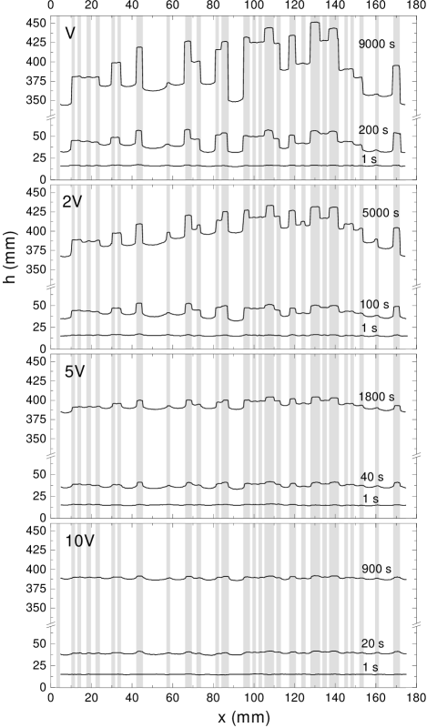
Figure 11: Sequence of interfaces for disorder T 1.50 and gap spacing $b=0.36$ mm, at different velocities, corresponding to Ca’=$1.62$, $3.25$, $8.13$, and $16.3$. The disorder pattern is shown in grey.

As discussed before, having tracks impedes that the interface gets locally pinned. As a result, the metastabilities observed for disorder SQ are not present here. Most of the fluctuations of $W(t)$ disappear, as shown in Fig. 12 for the four velocities studied. All the curves have approximately the same growth exponent $\beta=0.52\pm 0.03$. The transition from the growth regime to the saturation regime is rather smooth and makes it difficult to measure the values of $t_{\times}$ and $W_{s}$. Although two identical runs (with the same disorder configuration) give almost identical $W(t)$ curves, different disorder configurations give curves with slightly different $\beta$, $t_{\times}$, and $W_{s}$. In the former case the values vary between $\beta=0.48$ and $\beta=0.55$. The fluctuations observed at saturation are attributed to small inhomogeneities in the gap thickness, which affect particularly the experiments at the lowest velocities. Although the amplitude of the fluctuations decreases when we increase the number of disorder configurations, the almost perfect reproducibility of experiments with identical disorder configuration makes it difficult to have good statistics using a reduced number of disorder configurations.

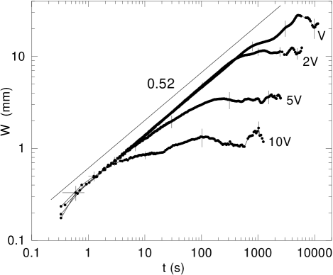
Figure 12: Interfacial width, $W(t)$, for disorder T 1.50, gap spacing $b=0.36$ mm, and four different velocities. The straight line drawn to guide the eye is the power law $W\sim t^{0.52}$.

The analysis of the power spectrum for the four velocities is shown in Fig. 13. The deterministic character of the interfacial growth makes the interfacial fluctuations not self–averaging. This leads to considerable fluctuations in the power spectrum, that cannot be completely reduced without using a large number of disorder configurations. Qualitatively, the power spectrum presents the same behaviour observed for SQ, with two different regimes separated by a crossover point $q_{c}$. The roughness exponent $\alpha_{1}$ increases with the velocity, varying from $\alpha_{1}=0.5\pm 0.1$ (slope $-2.1\pm 0.1$) for velocity $V$ to $\alpha_{1}=1.2\pm 0.1$ (slope $-3.4\pm 0.1$) for velocity $10\,V$. We have observed that at high velocities $\alpha_{1}$ reaches the same limiting value as it was measured for SQ 1.50.

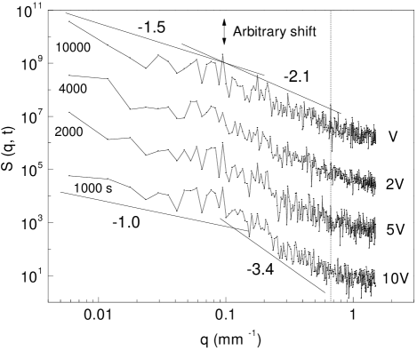
Figure 13: Determination of the roughness exponents from the power spectra for experiments at four different velocities, with $b=0.36$ mm and disorder T 1.50. The curves have been shifted in the vertical direction for clearness. The vertical line gives the value of $q$ associated with the spatial scale of the disorder. The other straight lines are power law fits from which the roughness exponents can be deduced.

VI.2 Variable gap spacing

VI.2.1 SQ 1.50 mm

Variations in the gap thickness modify the strength of the capillary forces in the vertical direction, which are destabilizing, in relation to the viscous forces and to the capillary forces in the plane of the cell, which are stabilizing. The sequence of interfaces at different $b$ and equal velocity ($2V$) of Fig. 14, indicate that roughening at large scales is inhibited for the smallest gap spacing, $b=0.16$ mm, and the interface remains globally flat. Notice that the oil–air interface adapts perfectly to the disorder configuration. The gap spacings must be increased to values larger than $b=0.23$ mm to observe all scales contributing to the roughening process.

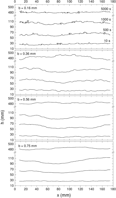
Figure 14: Sequence of interfaces at velocity $2V$ and disorder SQ 1.50, at different gap spacings corresponding to, from smaller to larger gap spacing, Ca’$=3.65$, $3.70$, $3.66$, and $3.62$. The disorder realization is the same in the four sequences. The reference velocity is $V=0.04$ mm/s.

The results of $W(t)$ for different gap spacings are presented in Fig. 15(a). The results show that the saturation times and widths are practically independent of gap spacing. This is a demonstration that increasing the gap thickness is not equivalent to increasing the velocity, although both changes result in larger Ca’. The growth exponent $\beta$ at the smallest gap spacings centers around $\beta=0.40$ but is subjected to a large error bar due to a significant presence of multivaluations in the interface. As $b$ increases there is a clear tendency towards a well defined power law, over three orders of magnitude in time, resulting in an exponent $\beta=0.50\pm 0.02$.

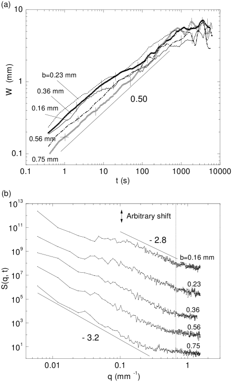
Figure 15: Experimental results at velocity $2V$ and disorder SQ 1.50 at five different gap spacings. a) Interfacial width $W(t)$. A power law with slope $0.5$ has been drawn to guide the eye. b) Power spectra at saturation ($t=6000$ s). The curves have been shifted in the vertical direction for clearness. The vertical line gives the value of $q$ associated with the spatial scale of the disorder.

Although all the experiments start with the same initial condition, the transition from an interface almost flat, with $W\simeq 0$, to a set of almost parallel $W(t)$ curves, suggest that the growth at very short times is strongly dependent on gap thickness.

The different role of velocity and gap spacing is also apparent from the power spectrum of the interfaces at saturation, shown in Fig. 15(b). For the smallest gap spacing, $b=0.16$ mm, the spectrum is nearly flat at small $q$, reflecting that the largest scales do not grow (Fig. 14). The only contribution to this part of the spectrum comes from the memory of the global shape of the initial front, which, at the smallest gap spacings, cannot be prepared perfectly flat. The power law dependence at larger $q$ extends from $q_{c}\simeq 0.15$ to $q=0.67$ (which corresponds to the lateral size of the disorder cell). As $b$ increases, the nearly $q$–independent behaviour at small $q$ changes to a power law behaviour (exponent $\alpha_{1}$), and the crossover value $q_{c}$ shifts to smaller $q$. For gap spacings as large as $b=0.75$ mm this shift leads to a single power law dependence, that could be strongly affected by finite–size effects. The measured exponents in the short length scale regime increase with $b$, from $\alpha_{1}=0.9\pm 0.1$ (slope $-2.8\pm 0.2$) to $\alpha_{1}=1.1\pm 0.1$ (slope $-3.2\pm 0.2$).

VI.2.2 T 1.50 mm

The gap spacing has been varied in the range $0.16\leqslant b\leqslant 0.75$, keeping the velocity fixed at $2V$. Fig. 16 show a sequence of the temporal evolution of the interfaces for four different gap spacings. The most remarkable aspect is the significant difference in the shape of the interfaces between $b=0.16$ mm and the other gap spacings. For $b=0.16$ mm the capillary forces are strong enough to inhibit correlations between neighbouring tracks. Similarly to the experiments with SQ 1.50 and the smallest gap, we do not expect saturation of scales larger than the average lateral size of the tracks. For $b\geqslant 0.36$ mm the behaviour is different: the interfacial height is correlated from the size of the basic disorder cell up to the system width. The interface at long length scales adopts a final shape at saturation identical for the three gaps, dominated by the spatial distribution of the disorder pattern. At short length scales the amplitude of the fingers depends on the relative strength of the capillary forces, tuned by the gap spacing.

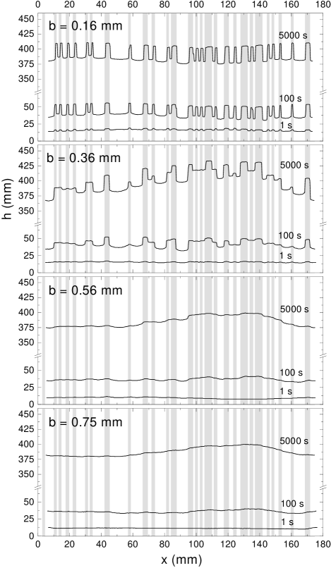
Figure 16: Sequence of interfaces at velocity $2V$ and disorder T 1.50, at different gap spacings corresponding to, from smaller to larger gap spacing, Ca’$=2.67$, $3.25$, $3.38$, and $3.41$.

Fig. 17(a) shows the $W(t)$ curves for the four gap spacings. The slopes are practically the same in all four cases, the saturation times are also very similar, and the saturation widths are progressively larger as the gap spacing is reduced. The fact that the interfacial fluctuations with $b=0.16$ mm reach saturation is a consequence of driving the system with a finite velocity that impedes an infinite deformation of the interface.

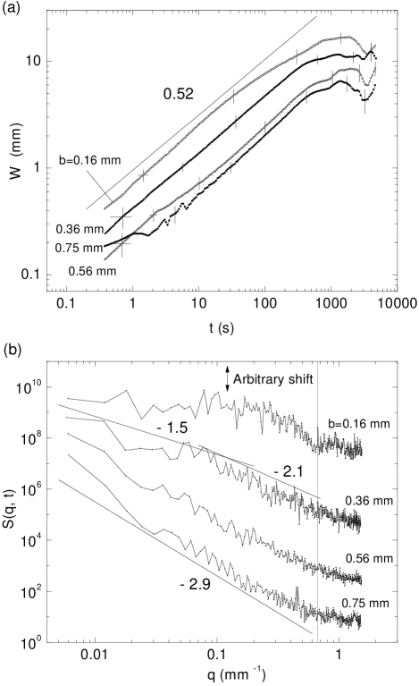
Figure 17: Experimental results at velocity $2V$ and disorder T 1.50, at four different gap spacings. a) Interfacial width $W(t)$. A power law with slope $0.52$ has been drawn to guide the eye. b) Power spectra at saturation ($t=6000$ s). The curves have been shifted in the vertical direction for clearness. The vertical line gives the value of $q$ associated with the spatial scale of the disorder.

In Fig. 17(b) we represent the spectra for the four velocities at saturation. The fact that for $b=0.16$ mm the interfacial height is uncorrelated for distances larger than the average lateral size of the tracks ($2.3$ mm, corresponding to $q=0.43$) is clearly observed, since for $q\lesssim 0.4$ we observe a plateau in the power spectrum. The only hint of a power law regime is at large $q$, from $q\gtrsim 0.4$ to the limit given by the disorder size, an interval too short to measure any roughness exponent. The other gap spacings show qualitatively the same behaviour observed for SQ. The large $q$ saturate with an exponent $\alpha_{1}$ that is progressively larger as we increase the gap spacing, varying from $\alpha_{1}=0.5\pm 0.1$ (slope $-2.1\pm 0.2$) for $b=0.36$ mm to $\alpha_{1}=0.9\pm 0.1$ (slope $-2.9\pm 0.2$) for $b=0.75$ mm. The regime characterized by $\alpha_{2}$ is only identifiable for $b=0.36$ mm. For the other gap spacings, our results indicate that we have a unique power law over all length scales. Here again, however, the results for the largest gap spacings could be severely influenced by finite size effects.

VII Analysis and discussion

The variation of the roughness exponents with velocity and gap spacing, for SQ and T disorder configurations, is summarized in Fig. 18. We observe that $\alpha_{1}$ and $\alpha_{2}$ have opposite behaviours as the interface velocity increases.

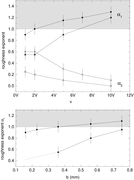
Figure 18: Variation of the roughness exponents with interface velocity (top) and gap spacing (bottom), for SQ 1.50 (circles) and T 1.50 (triangles). Solid and open symbols correspond to $\alpha_{1}$ and $\alpha_{2}$, respectively. The region of super–rough interfaces ($\alpha>1$) is shown in grey. The lines are drawn to guide the eye.

The exponent $\alpha_{1}$, characteristic of roughening at short length scales, increases with $v$. It becomes larger than $1$ (super–rough interface) already at moderate velocities. To understand this behaviour, we refer to Fig. 9(a), where it is shown that $\alpha_{1}$ is large at very short times, and decreases progressively as time goes on, at velocity $2V$. The initial super–roughness is due to the initially local dynamics of the interface fluctuations as the interface gets in contact with the disorder for the first time. At sufficiently large velocities, however, the subsequent decrease of $\alpha_{1}$ is not observed, and the initial super–roughness gets frozen in. The reason is that the saturation time $t_{\times}$ is comparable to the average time spent by the interface to go across the distance $\widetilde{l}$ (the average length of the disorder in the $y$ direction), estimated as $\tau=\widetilde{l}/v$. For example, for SQ 1.50, $b=0.36$ mm and $v=10\,V$, we have $t_{\times}=5$ s and $\tau=\widetilde{l}/v\simeq 6$ s. This explains also that $\alpha_{1}$ takes similar values for SQ and T at high velocities, since whenever $t_{\times}\simeq\tau$ the continuity of the disorder in the $y$ direction is irrelevant. In particular, we have evidence that $\alpha_{1}$ becomes identical for SQ and T at very large velocities. The interface is saturated at all time, making the interfacial dynamics in SQ equivalent to an average of the dynamics over a number of T configurations. For gap spacings around $b=0.36$ mm, we have observed that this condition is satisfied for $v\gtrsim 13V$. An identical value $\alpha_{1}\simeq 1.3$ has been obtained for both SQ and T by performing experiments at $30V$ ($t_{\times}\ll\tau$). This value of $\alpha_{1}$ is distinctively larger than previous experimental results, and coincides within error bars with the value $1.25$ found numerically in Ref. Dube-teoric-00 taking account of the nonlinearities. A super–rough interface ($\alpha>1$) is also obtained by scaling analysis in Aurora-EPL-01 , but with a larger exponent.

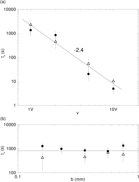
Figure 19: Saturation time $t_{\times}$ as a function of velocity $v$ (top) and gap spacing $b$ (bottom), for SQ 1.50 (circles) and T 1.50 (triangles). The straight lines have been drawn to guide the eye.

The exponent $\alpha_{2}$ (long length scales) measured in our experiments decreases with $v$. Its actual behaviour, however, could be obscured by finite size effects. The reason is that nonlocal effects on the interfacial dynamics (due to the fluid flow from the reservoir) become progressively more significant as $v$ increases. For experimental reasons we have not studied finite size effects in any systematic way. However, we do have checked that experiments performed at velocity $V$ and system size $L/2$ give the same exponent $\alpha_{2}$ than those at velocity $2V$ and system size $L$. The simultaneous dependence of $\alpha_{2}$ on velocity and system size can be estimated from $W(t)$ for both SQ and T. We have observed (Figs. 19(a) and 20(a)) that the saturation time $t_{\times}$ and the saturation width $W_{s}$ are power laws of the velocity $v$, of the form $t_{\times}\sim v^{-\delta}$ and $W_{s}\sim v^{-\gamma}$, with $\delta\simeq 2.5$ and $\gamma\simeq 1.1$ for SQ, and $\delta\simeq 2.3$ and $\gamma\simeq 1.2$ for T. Combining these relations with the FV scaling assumption (2), and taking into account that the saturation times and widths correspond to the long time regime (long length scales), we get:

$$\alpha_{2}\sim-\beta\delta\frac{\log v}{\log L},$$ (20)

with $\gamma=\beta\delta$. Given that the system size $L$ has been kept fixed in the experiments, the relation (20) predicts that the roughness exponent $\alpha_{2}$ obtained from the experiments will depend on $v$. The validity of this result is confirmed in Fig. 21, where the values of $\alpha_{2}$ are plotted vs. $\log v$.

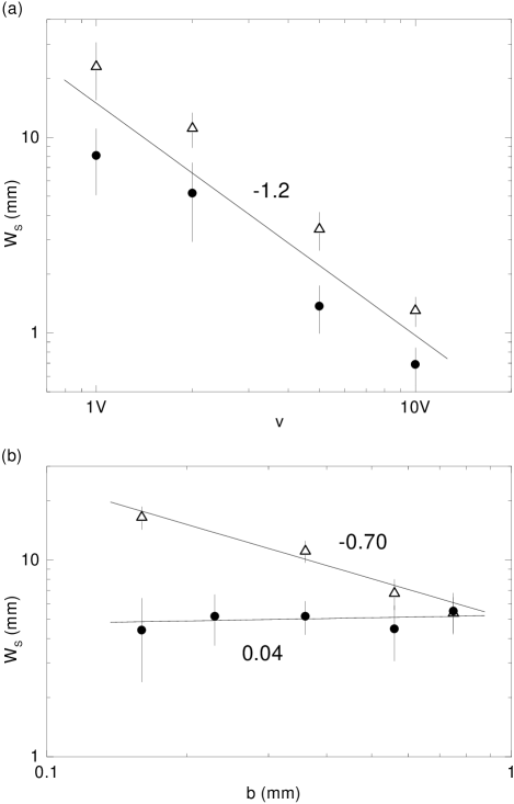
Figure 20: Saturation width $W_{s}$ as a function of velocity $v$ (top) and gap spacing $b$ (bottom), for SQ 1.50 (circles) and T 1.50 (triangles). The straight lines have been drawn to guide the eye.

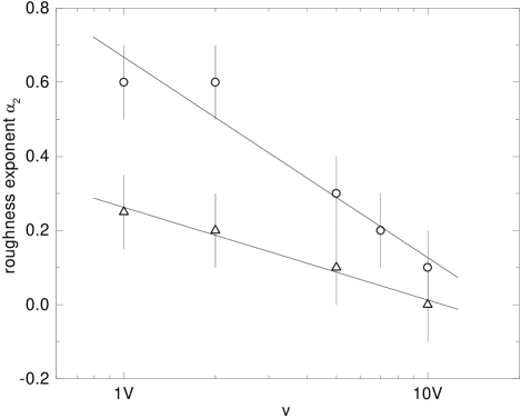
Figure 21: Roughness exponent $\alpha_{2}$ as a function of $\log v$ for SQ 1.50 (circles) and T 1.50 (triangles). The straight lines have been drawn to guide the eye.

From the observation that the difference between $\alpha_{1}$ and $\alpha_{2}$ decreases as $v$ is reduced (Fig. 18), and taking into account that capillary forces become also more important, we argue that in the limit of very low velocities the power spectrum would display an unique power law extending over all scales with a roughness exponent in the interval $0.6-0.9$, compatible with the observations in he-92 ; Rubio-89 ; Horvath-90 ; Rubio-90 ; Horvath-91 . This limit is unreachable for SQ because at velocities $v\lesssim V/2$ the interface gets locally pinned and develops overhangs. In the case of T there is no pinning or multivaluation, but the interface stretches to such a point that easily pinches off at long times, before saturation. These and other questions, present only in the regime of flows dominated by capillary forces, are studied in Ref. Soriano-2001-II .

Concerning the influence of $b$, the gap spacing, two main effects must be taken into account. First, the mobility is proportional to $b^{2}$ and hence increases with $b$, enhancing the stabilizing effect of the viscous pressure field (on long length scales) and the interfacial tension in the plane of the cell (on short length scales). Second, increasing $b$ weakens the destabilizing effect of the capillary forces induced by the disorder, which act on short length scales. The overall result is that the curves $W(t)$ are shifted towards smaller widths as $b$ increases, as shown in Figs. 15(a) and 17(a). The shift is such that $W\cdot b$ collapses the curves for different gap spacings into a single one, in both SQ and T cases. The fact that large values of $b$ makes the presence of the disorder irrelevant can be observed through the values of the roughness exponents $\alpha$, which show a tendency to converge into a single value $\alpha\simeq 1$ at large gap spacings and for any disorder configuration.

Another observation is that the saturation regime is reached always at almost the same saturation time $t_{\times}$, independently of the gap spacing, as Fig. 19(b) reveals. The interfacial width at saturation, however, has a different origin depending on gap spacing. For small $b$ the width is due to fluctuations at the shortest length scales, while for large $b$ it is due to fluctuations at longer length scales. This can be observed on the interfaces and is clearly reflected on the power spectrum (Figs. 15(b) and 17(b)). The passage from short to long length scales is continuous with $b$. It can be shown that replacing the variable $q$ by the dimensionless variable $q\cdot b$, produces the collapse of the power law region of the power spectra in Fig. 15(b).

Disorder	Low Ca’		Moderate Ca’		Large Ca’
	($\lesssim 3$)		($3<$ Ca’ $<10$		($\gtrsim 10$)
	$\alpha_{1}$	$\alpha_{2}$	$\alpha_{1}$	$\alpha_{2}$	$\alpha_{1}$	$\alpha_{2}$
SQ 1.50	$0.6-0.9$	$\--$	$\simeq 1$	$\simeq 0.6$	$\simeq 1.3$	$\simeq 0$
SQ-n 1.50	$0.6-0.9$	$\--$	$\simeq 0.9$	$\simeq 0.5$	$\simeq 1.3$	$\simeq 0$
T 0.40	New regime		$\simeq 0.7$	$\simeq 0.5$	$\simeq 1.3$	$\simeq 0$
T 1.50	New regime		$\simeq 0.5$	$\simeq 0.2$	$\simeq 1.3$	$\simeq 0$

Table 2: Summary of the values of the roughness exponents.

Table 2 shows the main results obtained for the roughness exponents $\alpha_{1}$ (short length scales) and $\alpha_{2}$ (long length scales) at different disorder configurations and drivings. For small Ca’, capillary forces are dominant at all scales, and the dynamics is very sensitive to the disorder configuration. For SQ and SQ-n, the interfaces get locally pinned, and the measured exponents are close to those obtained in DPD or in experiments where capillary forces are dominant he-92 ; Rubio-89 ; Horvath-90 ; Rubio-90 ; Horvath-91 . In the limit of persistent disorder, the nature of the disorder impedes pinning, but the effect of the destabilizing capillary forces combined with the correlations between neighboring tracks leads to a new regime that can be described using the anomalous scaling ansatz Soriano-2001-II . This new regime also extends to the region of moderate Ca’ for T disorder. For moderate Ca’, viscous forces are dominant at long length scales and two clear regimes separated by a crossover wavenumber $q_{c}$ can be characterized. For SQ and SQ-n we get roughness exponents $\alpha_{1}\gtrsim 1$ and $\alpha_{2}\simeq 0.5-0.6$. For T, we get a qualitatively similar behaviour, but obtaining lower values of the exponents due to finite size effects at long length scales and the dominant capillary forces at short length scales. For large Ca’, the viscous forces cause that the initial super–roughness at short times and short length scales gets frozen in, obtaining the same roughness exponent $\alpha_{1}\simeq 1.3$ for all the disorder configurations.

Our experimental results can be compared now with the predictions of the nonlocal models ganesan-98 ; Dube-teoric-99 ; Dube-teoric-00 ; Aurora-EPL-01 discussed in Section II. It appears that none of the models can account for the different results obtained in the whole range of capillary numbers explored. Although the Flory–type argument used by Ganesan and Brenner ganesan-98 is difficult to justify in this nonequilibrium situation, they obtain roughness exponents ($\alpha_{1}=3/4$ and $\alpha_{2}=1/2$) consistent with our values for small and moderate Ca’. The exponents obtained by Hernández–Machado et al. Aurora-EPL-01 for the long length scales at moderate Ca’, $\alpha_{2}=1/2$ and $z=1$ ($\beta_{2}=1/2$), are in agreement with our experimental values in the long time regime, where the viscous forces are dominant. The value of $\alpha$ for short length scales, corresponding to the short time regime of the model, gives a super–rough behaviour ($\alpha_{1}>1$) dominated by surface tension in the plane, but larger than the exponent measured in the experiment. For large capillary numbers the numerical result of Dubé et al. Dube-teoric-99 ; Dube-teoric-00 , $\alpha_{1}=1.3$, is in agreement with our experimental results, but not the result $\beta_{1}=0.3$ because, as pointed out above, these authors assume a spontaneous imbibition. At this point it would be interesting to know whether a model containing a quenched disorder both in the mobility and in the chemical potential would be able to explain the experimental results for the whole regime of Ca’ studied here, and specially the regime of large Ca’ in forced imbibition. This remains an open question.

Our last analysis is the variation of $q_{c}$ with $v$. The crossover wavenumber $q_{c}$ separates the regime in which the long length scale fluctuations (small $q$) are damped by the viscous pressure field, from the regime in which the short length scale fluctuations (large $q$) are damped by the interfacial tension in the plane of the cell. Since the relative importance of the viscous pressure field increases with Ca’, it is expected that $q_{c}$ will increase with $v$. Specifically, a linear analysis of the interfacial problem shows that the viscous damping is proportional to $v|q|$ and the interfacial tension damping is proportional to $q^{2}|q|$, which results in $q_{c}\propto v^{0.5}$ Dube-teoric-00 ; Aurora-EPL-01 .

In Fig. 22 we show the behaviour of $q_{c}$ with $v$ for different kinds of disorder. The error bars are relatively large because the exact location of $q_{c}$ in the experimental power spectra is difficult to ascertain. For SQ 1.50 we find that $q_{c}\propto v^{0.47}$, in good agreement with the theoretical prediction. It is interesting to note that, as we go to disorders of larger $\widetilde{l}$ (increasing persistence), $q_{c}$ tends to be less sensitive to $v$. For T 1.50 we observe that $q_{c}$ becomes independent of $v$, within error bars. The reason can be understood in the framework of the following scenario: at a local level (see Fig. 1) the motion of the interface in the SQ disorder can be viewed as a series of events formed by a period of nearly steady motion, a subsequent period of fast advance over a copper island (accompanied by an abrupt change of sign of the in–plane curvature), and a third period of fast advance over fiber–glass due to relaxation of the local in–plane curvature. Thus, damping of the short length scales due to the interfacial tension in the plane of the cell is basically effective only in this last period, when the interface depins from the copper islands. As the persistence of the disorder in the $y$ direction is larger, the relaxation periods are less frequent. This can be observed through the histogram of Fig. 4. When we increase the persistence of the disorder changing from SQ to SQ-n, the number of the smallest copper aggregations reduces almost one order of magnitude. In the limiting case of T 1.50 the disorder is continuous in the $y$ direction, and the damping role of the in–plane interfacial tension is effectively suppressed.

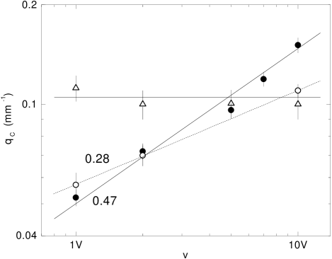
Figure 22: Dependence of the crossover wavenumber $q_{c}$ on velocity $v$ for three disorder configurations: SQ 1.50 (solid circles), SQ-n 1.50 (open circles) and T 1.50 (triangles).

VIII Conclusions

We have presented new experiments of forced fluid imbibition in a Hele–Shaw cell with quenched disorder. We have used three main kinds of disorder patterns, SQ, SQ-n and T, characterized by an increasing persistence length $\widetilde{l}$ in the direction of growth. We have measured a robust roughness exponent $\beta\simeq 0.5$ that is almost independent of the disorder configuration, interface velocity, and gap spacing, although the behaviour of the interfacial width presents important fluctuations both during growth and at saturation, that progressively disappear as the disorder is more persistent in the $y$ direction. The roughness exponent $\alpha$, however, shows a clear dependence on the experimental parameters, as summarized in Table 2, discussed in the previous Section. Finally, we have focused on the dependence of the crossover wavenumber as a function of the interface velocity $v$ and $\widetilde{l}$. For the shortest $\widetilde{l}$, $q_{c}\sim v^{0.47}$, and becomes independent of $v$ as the disorder is persistent in the $y$ direction.

The absence of pinning in experiments with disorders of increasing $\widetilde{l}$ allows a detailed investigation of the regime of large capillary forces. This regime presents some interesting novel features which are studied in detail in Ref. Soriano-2001-II .

IX Acknowledgements

We are grateful to M. A. Rodríguez, L. Ramírez-Piscina, J. Casademunt, K. J. Måløy, and J. Schmittbuhl for fruitful discussions. The research has received financial support from the Dirección General de Investigación (MCT, Spain), project BFM2000-0628-C03-01. J. O. acknowledges the Generalitat de Catalunya for additional financial support. J. S. is supported also by a fellowship of the DGI (MCT, Spain).

References

- (1) A.-L. Barabási and H.E. Stanley, Fractal Concepts in Surface Growth, Cambridge University Press, Cambridge (1995).
- (2) J. Krug, Adv. Phys. 46, 139 (1997).
- (3) P. Meakin, Fractals, Scaling and Growth far from Equilibrium. Cambridge University Press, Cambridge, 1998.
- (4) P.-z. Wong, MRS Bull. 19, No. 5, 32 (1994), and references therein.
- (5) M. Dubé, M. Rost, and M. Alava, Eur. Phys. J. B 15, 691 (2000).
- (6) P.G. de Gennes, J. Phys. 47, 1541 (1986).
- (7) A. Paterson, M. Fermigier, P. Jenffer, and L. Limat, Phys. Rev. E 51, 1291 (1995); A. Paterson and M. Fermigier, Phys. Fluids 9, 2210 (1997).
- (8) F. Family and T. Vicsek, J. Phys. A 18, L75 (1985).
- (9) J.M. López and M.A. Rodríguez, Phys. Rev. E 54, R2189 (1996); J.M. López, M.A. Rodríguez, and R. Cuerno, Physica A 246, 329 (1997).
- (10) J.J. Ramasco, J.M. López, and M.A. Rodríguez, Phys. Rev. Lett. 84, 2199 (2000).
- (11) M. Kardar, G. Parisi, and Y.C. Zhang, Phys. Rev. Lett. 56, 889 (1986).
- (12) S.F. Edwards and D.R. Wilkinson, Proc. R. Soc. London A 381, 17 (1982).
- (13) H. Leschhorn, Phys. Rev. E 54, 1313 (1996); H. Leschhorn, T. Nattermannn, S. Stepanow, and L.-H. Tang, Ann. Phys. 6, 1 (1997).
- (14) J. Krug and P. Meakin, Phys. Rev. Lett. 66, 703 (1991).
- (15) S. He, G. L. M. K. S. Kahanda, and P.Z. Wong, Phys. Rev. Lett. 69, 3731 (1992).
- (16) V. Ganesan and H. Brenner, Phys. Rev. Lett. 81 578, (1998).
- (17) A. Hernández–Machado, J. Soriano, A.M. Lacasta, M.A. Rodríguez, L. Ramírez–Piscina, and J. Ortín, Europhys. Lett. 55, 194 (2001).
- (18) M. Dubé, M. Rost, K.R. Elder, M. Alava, S. Majaniemi, and T. Ala-Nissila, Phys. Rev. Lett. 83 1628 (1999).
- (19) M. Dubé, M. Rost, K.R. Elder, M. Alava, S. Majaniemi, and T. Ala-Nissila, Eur. Phys. J. B 15, 701 (2000).
- (20) M.A. Rubio, C.A. Edwards, A. Dougherty, and J.P. Gollub, Phys. Rev. Lett. 63, 1685 (1989).
- (21) V.K. Horváth, F. Family, and T. Vicsek, Phys. Rev. Lett. 65, 1388 (1990).
- (22) M.A. Rubio, A. Dougherty, and J.P. Gollub, Phys. Rev. Lett. 65, 1389 (1990).
- (23) V.K. Horváth, F. Family, and T. Vicsek, J. Phys. A 24, L25 (1991).
- (24) V.K. Horváth, F. Family, and T. Vicsek, Phys. Rev. Lett. 67, 3207 (1991).
- (25) A. Dougherty and N. Carle, Phys. Rev. E 58, 2889 (1998).
- (26) M. Avellaneda and S. Torquato, Phys. Fluids A 3, 2529 (1991).
- (27) A. Koponen, M. Kataja, and J. Timonen. Phys. Rev. E 54, 406 (1996).
- (28) A. Koponen, M. Kataja, and J. Timonen. Phys. Rev. E 56, 3319 (1997).
- (29) G.M. Homsy, Ann. Rev. Fluid Mech. 19, 271 (1987).
- (30) I. Simonsen, A. Hansen, and O. M. Nes, Phys. Rev. E 58, 2779 (1998).
- (31) J. Schmittbuhl, J.-P. Vilotte, and S. Roux, Phys. Rev. E 51, 131 (1995).
- (32) G. Tripathy and W. van Saarloos. Phys. Rev. Lett. 85, 3556 (2000).
- (33) J. Soriano, J.J. Ramasco, M.A. Rodríguez, A. Hernández-Machado, and J. Ortín, Phys. Rev. Lett. 89, 026102 (2002); J. Soriano, J. Ortín, and A. Hernández-Machado, to be published.