Synapse efficiency diverges due to synaptic pruning following over-growth

Abstract

In the development of the brain, it is known that synapses are pruned following over-growth. This pruning following over-growth seems to be a universal phenomenon that occurs in almost all areas – visual cortex, motor area, association area, and so on. It has been shown numerically that the synapse efficiency is increased by systematic deletion. We discuss the synapse efficiency to evaluate the effect of pruning following over-growth, and analytically show that the synapse efficiency diverges as $O(|\log c|)$ at the limit where connecting rate $c$ is extremely small. Under a fixed synapse number criterion, the optimal connecting rate, which maximize memory performance, exists.

I Introduction

In this paper, we analytically discuss synapse efficiency to evaluate effects of pruning following over-growth during brain development, within the framework of auto-correlation-type associative memory.

Because this pruning following over-growth seems to be a universal phenomenon that occurs in almost all areas – visual cortex, motor area, association area, and so on Huttenlocker1979 ; Huttenlocker1982 ; Bourgeois1993 ; Takacs1986 ; Innocenti1995 ; Eckehoff1991 ; Rakic1994 ; Stryker1986 ; Sur1990 ; Wolff1995 – we discuss the meaning of its function from a universal viewpoint rather than in terms of particular properties in each area. Of course, to discuss this phenomenon as a universal property of a neural network model, we need to choose an appropriate model.

Artificial neural network models are roughly classified into two types: feed forward models and recurrent models. Various learning rules are applied to the architectures of these models, and correlation learning corresponding to the Hebb rule can be considered a prototype of any other learning rules. For instance, correlation learning can be regarded as a first-order approximation of the orthogonal projection matrix, because the orthogonal projection matrix can be expanded by correlation matrices Yanai1996 . In this respect, we can naturally regard a correlation-type associative memory model as one prototype of the neural network models of the brain. For example, Amit et al. discussed the function of the column of anterior ventral temporal cortex by means of a model based on correlation-type associative memory model Amit1994 ; Griniasty1993 . Also, Sompolinsky discussed the effect of dilution. He assumed that the capacity is proportional to the number of remaining bonds, and pointed out that a synapse efficiency of diluted network, which is storage capacity per a connecting rate, is higher than a full connected network’s one Sompolinsky1986b . Chechik et al. discussed the significance of the function of the pruning following over-growth on the basis of a correlation-type associative memory model Chechik1998 . They pointed out that a memory performance, which is stored pattern number per synapse number, is maximized by systematic deletion that cuts synapses that are lightly weighted. However, while it is qualitatively obvious that synapse efficiency and memory performance are increased by a systematic deletion, we also need to consider the increase of synapse efficiency quantitatively.

In this paper, we quantitatively compare the effectiveness of systematic deletion to that with random deletion on the basis of an auto-correlation-type associative memory model. In this model, one neuron is connected to other neurons with a proportion of $c$, where $c$ is called the connecting rate. Systematic deletion is considered as a kind of nonlinear correlation learning Okada1998 . At the limit where the number of neurons $N$ is extremely large, it is known that random deletion and nonlinear correlation learning can be transformed into correlation learning with synaptic noise Sompolinsky1986b ; Okada1998 . These two types of deletion, systematic and random, are strongly related to multiplicative synaptic noise. First, we investigated the dependence of storage capacity on multiplicative synaptic noise. At the limit where multiplicative synaptic noise is extremely large, we show that storage capacity is inversely proportional to the variance of the multiplicative synaptic noise. From this result, we analytically derive that the synapse efficiency in the case of systematic deletion diverges as $O(|\log c|)$ at the limit where the connecting rate $c$ is extremely small. We also show that the synapse efficiency in the case of systematic deletion becomes $2|\log c|$ times as large as that of random deletion.

In addition to such the fixed neuron number criterion as the synapse efficiency, a fixed synapse number criterion could be discussed. At the synaptic growth stage, it is natural to assume that metabolic energy resources are restricted. When metabolic energy resources are limited, it is also important that the effect of synaptic pruning is discussed under limited synapse number. Under this criterion, the optimal connecting rate, which maximize memory performance, exists. These optimal connecting rates are in agreement with the computer simulation results given by Chechik et al Chechik1998 .

II Model

Sompolinsky discussed the effects of synaptic noise and nonlinear synapse by means of the replica method Sompolinsky1986b . However, symmetry of the synaptic connections $J_{ij}=J_{ji}$ is required in the replica method since the existence of the Ljapunov function is necessary. Therefore, there was a problem that the symmetry regarding synaptic noise had to be assumed in the Sompolinsky theory. To avoid this problem, Okada et al. discussed additive synaptic noise, multiplicative synaptic noise, random synaptic deletion, and nonlinear synapse by means of the self-consistent signal-to-noise analysis (SCSNA) Okada1998 . They showed that additive synaptic noise, random synaptic deletion, nonlinear synapse can be transformed into multiplicative synaptic noise.

Here, we discuss the synchronous dynamics as,

$$x_{i}=F(\sum_{j\neq i}^{N}J_{ij}x_{j}+h),$$ (1)

where $F$ is the response function, $x_{i}$ is the output activity of neuron $i$, and $-h$ is the threshold of each neuron. Every component $\xi_{i}^{\mu}$ in a memorized pattern $\mbox{\boldmath$\xi$}^{\mu}$ is an independent random variable,

$${\rm Prob}[\xi_{i}^{\mu}=\pm 1]=\frac{1\pm a}{2},$$ (2)

and the generated patterns are called sparse pattern with bias $a\;(-1<a<1)$. We have determined that the firing rate of states in the retrieval phase is the same for each memorized pattern Amit1987 ; Amari1989 . In this case, threshold $-h$ can be determined as,

$$a=\frac{1}{N}\sum_{i=1}^{N}\mbox{sgn}(\sum_{j\neq i}J_{ij}x_{i}+h).$$ (3)

The firing rate becomes $f=(1+a)/2$ at the bias $a$.

Additive synaptic noise, multiplicative synaptic noise, random synaptic deletion, and nonlinear synapse can be introduced by synaptic connections in the following manner.

In the case of additive synaptic noise, synaptic connections are constituted as,

$$J_{ij}=\frac{J}{N(1-a^{2})}\sum_{\mu=1}^{\alpha N}(\xi_{i}^{\mu}-a)(\xi_{j}^{\mu}-a)+\delta_{ij},$$ (4)

where $\delta_{ij}$ is the additive synaptic noise. The symmetric additive synaptic noise $\delta_{ij}$ and $\delta_{ji}$ are generated according to the probability,

$$\delta_{ij}\sim N(0,\frac{\delta_{A}^{2}}{N}),\quad\delta_{ij}=\delta_{ji},$$ (5)

where $\delta_{A}^{2}$ is the absolute strength of the additive synaptic noise. The parameter $\delta_{A}$ is assumed to be $O(1)$. This means that the synaptic connection $J_{ij}$ is $O(1/\sqrt{N})$. It is useful to define the parameter $\Delta_{A}$ as

$$\Delta_{A}\equiv\frac{\delta_{A}}{J/(1-a^{2})},$$ (6)

which measures the relative strength of the noise and we call the parameter $\Delta_{A}^{2}$ the variance of the additive synaptic noise. Therefore, we define the probability to generate the additive synaptic noise $\delta_{ij}$ as

$$\delta_{ij}\sim N(0,\frac{J^{2}}{N(1-a^{2})^{2}}\Delta_{A}^{2}),\quad\delta_{ij}=\delta_{ji}.$$ (7)

In the case of multiplicative synaptic noise, synaptic connections are constituted as,

$$J_{ij}=\frac{1+\varepsilon_{ij}}{N(1-a^{2})}\sum_{\mu=1}^{\alpha N}(\xi_{i}^{\mu}-a)(\xi_{j}^{\mu}-a),$$ (8)

where $\varepsilon_{ij}$ is multiplicative synaptic noise. The symmetric multiplicative noise $\varepsilon_{ij}$ and $\varepsilon_{ji}$ are generated according to the probability,

$$\varepsilon_{ij}\sim N(0,\Delta_{M}^{2}),\quad\varepsilon_{ij}=\varepsilon_{ji},$$ (9)

where $\Delta_{M}^{2}$ is the variance of the multiplicative synaptic noise.

In the model of random synaptic deletion, synaptic connections are constituted as,

$$J_{ij}=\frac{c_{ij}}{Nc(1-a^{2})}\sum_{\mu=1}^{\alpha N}(\xi_{i}^{\mu}-a)(\xi_{j}^{\mu}-a),$$ (10)

where $c_{ij}$ is a cut coefficient. The synapse that is cut is represented by the cut coefficient $c_{ij}=0$. In the case of symmetric random deletion, the cut coefficients $c_{ij}$ and $c_{ji}$ are generated according to the probability,

$$\mbox{Prob}[c_{ij}=1]=1-\mbox{Prob}[c_{ij}=0]=c,\quad c_{ij}=c_{ji},$$ (11)

where $c$ is the connecting rate.

In the model of nonlinear synapse, synaptic connections are constituted as,

$$J_{ij} = \frac{\sqrt{p}}{N}f(T_{ij}),$$ (12)

$$T_{ij} = \frac{1}{\sqrt{p}(1-a^{2})}\sum_{\mu=1}^{p}(\xi_{i}^{\mu}-a)(\xi_{j}^{\mu}-a)$$ (13)

$$\sim N(0,1),$$

where $p=\alpha N$. The nonlinear synapse is introduced by applying the nonlinear function $f(x)$ to the conventional Hebbian connection matrix $T_{ij}$.

II.1 Systematic deletion by nonlinear synapse

Chechik et al. pointed out that a memory performance, which is a storage pattern number per a synapse number, is maximized by systematic deletion that cuts synapses that are lightly weighted Chechik1998 ; Amit1994 ; Griniasty1993 . Such a systematic deletion can be represented by the nonlinear function $f(x)$ for a nonlinear synapse. In accordance with Chechik et al., we discuss three types of nonlinear functions (Figs.1, 2, and 3). Fig.1 shows clipped modification that is discussed generally as

$$f_{1}(z,t)=\left\{\begin{array}[]{ll}\mbox{sgn}(z),&|z|>t\\ 0,&\mbox{otherwise}.\end{array}\right.$$ (14)

Chechik et al. also obtained the nonlinear functions shown in Figs.2 and 3 by applying the following optimization principles Chechik1998 ; Meilijson1996 . In order to evaluate the effect of synaptic pruning on the network’s retrieval performance, Chechik et al. study its effect on the signal-to-noise ratio (S/N) of the internal field $h_{i}\equiv\sum_{j\neq i}J_{ij}x_{j}+h$ Chechik1998 . The S/N is calculated by analyzing the moments of the internal field and was given as

$$S/N = \frac{E[h_{i}|\xi_{i}^{\mu}=1]-E[h_{i}|\xi_{i}^{\mu}=-1]}{\sqrt{V[h_{i}|\xi_{i}^{\mu}]}}$$ (15)

$$\propto \frac{E[zf(z)]}{\sqrt{E[f(z)^{2}]}}=\frac{\displaystyle{\int_{-\infty}^{\infty}Dz\;zf(z)}}{\displaystyle{\int_{-\infty}^{\infty}Dz\;f(z)^{2}}}$$

$$\equiv \rho(f(z),z),$$

where $z$ has standard normal distribution, i.e., $E[z^{2}]=V[z]=1$ and $Dz$ is Gaussian measure defined as

$$Dz=\frac{dz}{\sqrt{2\pi}}\exp(-\frac{z^{2}}{2}),$$ (16)

and $E,V$ denote the operators to calculate the expectation and the variance for the random variables $\xi_{i}^{\mu}\;(i=1,\cdots,N,\mu=1,\cdots,\alpha N)$, respectively. The function $\rho(f(z),z)$ denotes the correlation coefficient. Chechik et al. considered the piecewise linear function like following nonlinear functions. In order to find the best nonlinear function $f(z)$, we should maximize $\rho(f(z),z)$, which is invariant to scaling. Namely, the best nonlinear function $f(x)$ is obtained by maximizing $E[zf(z)]$ under the condition that $E[f(z)^{2}]$ is constant. Let $\gamma$ be the Lagrange multiplier, it is sufficient to solve

$$\int_{-\infty}^{\infty}Dz\;zf(z)-\gamma\left(\int_{-\infty}^{\infty}Dz\;f(z)^{2}-c_{0}\right)\to\mbox{max},$$ (17)

for some constant $c_{0}$. Since the synaptic connection before acting the nonlinear function $T_{ij}$ obeys a Gaussian distribution $N(0,1)$, Eq.(13) is averaged over all of the synaptic connections.

Thus, the nonlinear function shown in Fig.2,

$$f_{2}(z,t)=\left\{\begin{array}[]{ll}z,&|z|>t\\ 0,&\mbox{otherwise},\end{array}\right.$$ (18)

is also obtained. The deletion by this nonlinear function is called minimal value deletion. Similarly, by adding the condition that the total strength of synaptic connection $\int Dz\;|f(z)|$ is constant, the nonlinear function

$$f_{3}(z,t) = \left\{\begin{array}[]{ll}z-\mbox{sgn}(z)t,&|z|>t\\ 0,&\mbox{otherwise}\end{array}\right.$$ (21)

$$= f_{2}(z,t)-tf_{1}(z,t),$$ (22)

is obtained. The deletion by this nonlinear function is called compressed deletion. We discuss systematic deletion by using these three types of nonlinear functions $f_{1}(z,t),f_{2}(z,t)$ and $f_{3}(z,t)$ given by Chechik et al Chechik1998 .

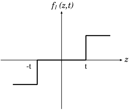
Figure 1: Clipped synapse.

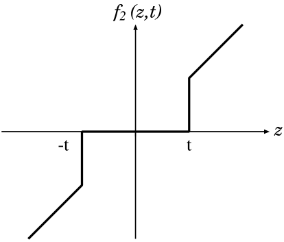
Figure 2: Minimal value deletion.

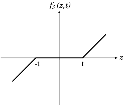
Figure 3: Compressed deletion.

III Results

In this section, the results concerning the multiplicative synaptic noise, the random deletion, and the nonlinear synapse are shown, at the limit where the effect of these deletions is extremely large.

The SCSNA starts from the fixed-point equations for the dynamics of an $N$-neuron network as Eq.(1). The results of the SCSNA for the symmetric additive synaptic noise are summarized by the following order-parameter equations (see Appendix A) :

$$m = \frac{1}{1-a^{2}}\int Dz<(\xi-a)Y(z;\xi)>_{\xi},$$ (23)

$$q = \int Dz<Y(z;\xi)^{2}>_{\xi},$$ (24)

$$U = \frac{1}{\sigma}\int Dz\;z<Y(z;\xi)>_{\xi},$$ (25)

$$\sigma^{2} = \frac{\alpha J^{2}q}{(1-JU)^{2}}+\frac{J^{2}}{(1-a^{2})^{2}}\Delta_{A}^{2}q.$$ (26)

$$Y(z;\xi) = F\biggl{(}J(\xi-a)m+\sigma z+h$$ (27)

$$+\biggl{[}\frac{\alpha J^{2}U}{1-JU}+\frac{J^{2}}{(1-a^{2})^{2}}\Delta_{A}^{2}\biggr{]}Y(z;\xi)\biggr{)},$$

where $<\cdots>_{\xi}$ implies averaging over the target pattern, $m$ is the overlap between the 1st memory pattern $\mbox{\boldmath$\xi$}^{1}$ and the equilibrium state $x$ is defined as

$$m=\frac{1}{N(1-a^{2})}\sum_{i=1}^{N}(\xi^{1}_{i}-a)x_{i},$$ (28)

note that generality is kept even if the overlap was defined by only the 1st memory pattern, $q$ is Edwards-Anderson order-parameter, $U$ is a kind of the susceptibility, which measures sensitivity of neuron output with respect to the external input, $Y(z;\xi)$ is effective response function, $\sigma^{2}$ is the variance of the noise. We set the output function $F(x)={\rm sgn}(x)-a$ in the following sections, where domain of the $x$ variable is $F(x)=1-a$ when $x\leq 0$, otherwise $F(x)=-1-a$.

According to Okada et al. Okada1998 , the symmetric additive synaptic noise, the symmetric random deletion, and the nonlinear synapse can be transformed into the symmetric multiplicative synaptic noise as follows (see Appendix B): the additive synaptic noise is

$$\Delta_{M}^{2}=\frac{\Delta_{A}^{2}}{\alpha(1-a^{2})^{2}},$$ (29)

the random deletion is

$$\Delta_{M}^{2}=\frac{1-c}{c},$$ (30)

and the nonlinear synapse is

$$\Delta_{M}^{2}=\frac{{\tilde{J}}^{2}}{J^{2}}-1,$$ (31)

where $J,\tilde{J^{2}}$ are

$$J = \int Dz\;zf(z),$$ (32)

$${\tilde{J}}^{2} = \int Dz\;f(z)^{2}.$$ (33)

In the following sections, symmetries of the additive synaptic noise, the multiplicative synaptic noise and random deletion are assumed. @ Storage capacity can be obtained by solving the order-parameter equations.

Figure 4 shows $m(\alpha)$ curves in the random deletion network with the number of neurons $N=3000$ and the firing rate $f=0.1$ for the connecting rate $c=0.1$,$c=0.3$, and $c=1.0$. It can be confirmed that the theoretical results of the SCSNA are in good agreement with the computer simulation results from Fig.4. Since it is known that theoretical results obtained by means of the SCSNA are generally in good agreement with the results obtained through the computer simulations using various models that include synaptic noise, we treat the results by means of the SCSNA only Shiino1992 ; Shiino1993 ; Okada1995 ; Okada1996 ; Okada1998 ; Mimura1998-1 ; Mimura1998-2 ; Kimoto2001 .

Through the relationships of Eqs.(29)-(33), the symmetric additive synaptic noise, the symmetric random deletion, and the nonlinear synapse can be discussed in terms of the symmetric multiplicative synaptic noise. Therefore, first of all, we deal with the multiplicative synaptic noise.

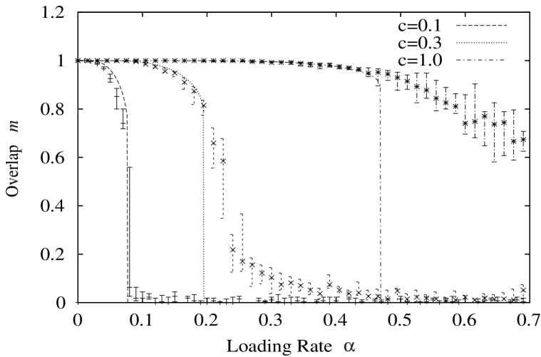
Figure 4: Overlaps in the random deletion network. The curves represent the theoritical results. The dots represent simulation results with $N=3000$ and $f=0.1$ for the connecting rate $c=0.1$,$c=0.3$, and $c=1.0$.

III.1 Multiplicative synaptic noise

Figure 5 shows the dependence of storage capacity on the multiplicative synaptic noise. As it is clear from Fig.5, storage capacity $\alpha_{c}$ is inversely proportional to the variance of the multiplicative synaptic noise $\Delta_{M}^{2}$, when the multiplicative synaptic noise is extremely large. Storage capacity $\alpha_{c}$ asymptotically approaches

$$\alpha_{c}=\frac{2}{\pi\Delta_{M}^{2}},$$ (34)

(see Appendix C). In the sparse limit where the firing rate is extremely small, it is known that storage capacity becomes $\alpha_{c}\simeq 1/(f|\log f|)$ Tsodyks1988 ; Amari1989 ; Buhmann1989 ; Perez-Vincente1989 ; Okada1996 .

Figure 5 shows the results from the SCSNA and the asymptote at the firing rate $f=0.5$. Figure 6 shows the results from the SCSNA at various firing rates. It can be confirmed that the order of the asymptote $O(\frac{1}{\Delta_{M}^{2}})$ does not depend on the firing rate from Fig.6.

Figure 5: Dependence of storage capacity $\alpha_{c}$ on the multiplicative synaptic noise $\Delta_{M}^{2}$ at the firing rate $f=0.5$. Comparison of asymptote and the results from the SCSNA.

Figure 6: Dependence of storage capacity $\alpha_{c}$ on the multiplicative synaptic noise $\Delta_{M}^{2}$. It can be confirmed that the order of the asymptote does not depend on the firing rate.

III.2 Random deletion

Next, we discuss the asymptote of the random deletion. The random deletion with the connecting rate $c$ can be transformed into the multiplicative synaptic noise by Eq.(30). Hence, at the limit where the connecting rate $c$ is extremely small, storage capacity becomes

$$\alpha_{c}=\frac{2}{\pi\Delta_{M}^{2}}=\frac{2c}{\pi(1-c)}\to\frac{2}{\pi}c,$$ (35)

according to the asymptote of the multiplicative synaptic noise in Eq.(34). In the random deletion, the synapse efficiency $S_{eff}$, which is storage capacity per the connecting rate Okada1998 ; Sompolinsky1986b , i.e., storage capacity per the input of one neuron, and defined as

$$S_{eff}\equiv\frac{\alpha_{c}}{c},$$ (36)

approaches a constant value as

$$S_{eff}=\frac{\alpha_{c}}{c}=\frac{2}{\pi},$$ (37)

according to Eq.(35) at the limit where the connecting rate $c$ is extremely small.

Figure 7 shows the result from the SCSNA and the asymptote at the firing rate $f=0.5$. Figure 8 shows the results from the SCSNA at various firing rates. It can be confirmed that the order of the asymptote, $O(1)$ with respect to $c$, does not depend on the firing rate from Fig.8.

Figure 7: Dependence of the synapse efficiency $S_{eff}$ on the random deletion with the connecting rate $c$ at the firing rate $f=0.5$. Comparison of asymptote and the results from the SCSNA.

Figure 8: Dependence of the synapse efficiency $S_{eff}$ on the random deletion with the connecting rate $c$ at various firing rates. It can be confirmed that the order of the asymptote does not depend on the firing rate.

III.3 Systematic Deletion

III.3.1 Clipped synapse

Synapses within the range $-t<z<t$ are pruned by the nonlinear function of Eq.(14).

The connection rate $c$ of the synaptic deletion in Eq.(13) is given by,

$$c = \int_{\{z|f_{1}(z,t)\neq 0\}}Dz=1-\mbox{erf}(\frac{t}{\sqrt{2}})$$ (38)

$$\to \sqrt{\frac{2}{\pi}}t^{-1}\exp(-\frac{t^{2}}{2}),\;\;t\to\infty,$$

since the synaptic connection $T_{ij}$ before acting the nonlinear function of Eq.(13) obeys the Gaussian distribution $N(0,1)$. Next, $J,\tilde{J}$ of Eqs.(32) and (33) become

$$J = 2\int_{t}^{\infty}Dz\;z\mbox{sgn}(z)=\sqrt{\frac{2}{\pi}}\exp(-\frac{t^{2}}{2})$$ (39)

$$\to tc,\;t\to\infty,$$

$${\tilde{J}}^{2} = 2\int_{t}^{\infty}Dz=1-\mbox{erf}(\frac{t}{\sqrt{2}})=c.$$ (40)

Hence, the equivalent multiplicative synaptic noise $\Delta_{M}^{2}$ is obtained as,

$$\Delta_{M}^{2}=\frac{{\tilde{J}}^{2}}{J^{2}}-1\to\frac{1}{t^{2}c},\;\;t\to\infty.$$ (41)

The relationship of the pruning range $t$ and the connecting rate $c$

$$t^{2}=-2\log c,$$ (42)

is obtained by taking the logarithm of Eq.(38) at $t\to\infty$ limit. Therefore, at the limit where the equivalent connecting rate $c$ is extremely small, storage capacity $\alpha_{c}$ can be obtained

$$\alpha_{c}=-\frac{4}{\pi}c\log c,$$ (43)

through Eqs.(34), (41), and (42). The synapse efficiency becomes

$$S_{eff}=\frac{\alpha_{c}}{c}=-\frac{4}{\pi}\log c.$$ (44)

Figure 9 shows the results from the SCSNA and the asymptote at the firing rate $f=0.5$. Figure 10 shows the results from the SCSNA at various firing rates. It can be confirmed that the order of the asymptote $O(\log c)$ does not depend on the firing rate from Fig.10.

Figure 9: Dependence of the synapse efficiency $S_{eff}$ with the clipped synapse on the connecting rate $c$ at $f=0.5$. Comparison of the results from the SCSNA and asymptote.

Figure 10: Dependence of the synapse efficiency $S_{eff}$ with the clipped synapse on the firing rate $f$. It can be confirmed that the order of the asymptote does not depend on the firing rate.

III.3.2 Minimal value deletion

In a similar way, the equivalent multiplicative synaptic noise $\Delta_{M}^{2}$ of the systematic deletion of Eq.(18) is obtained as follows,

$$\Delta_{M}^{2}=\frac{{\tilde{J}}^{2}}{J^{2}}-1\to\frac{1}{t^{2}c},\;\;t\to\infty.$$ (45)

where the connecting rate $c$ and $J,\tilde{J}$ of Eqs.(32) and (33) are

$$c = \int_{\{z|f_{2}(z,t)\neq 0\}}Dz=1-\mbox{erf}(\frac{t}{\sqrt{2}})$$ (46)

$$\to \sqrt{\frac{2}{\pi}}t^{-1}\exp(-\frac{t^{2}}{2}),\;\;t\to\infty,$$

$$J = \sqrt{\frac{2}{\pi}}t\exp(-\frac{t^{2}}{2})+1-\mbox{erf}(\frac{t}{\sqrt{2}})$$ (47)

$$\to \sqrt{\frac{2}{\pi}}t\exp(-\frac{t^{2}}{2}),\;\;t\to\infty,$$

$${\tilde{J}}^{2} = J,$$ (48)

respectively. Hence, at the limit where the equivalent connecting rate $c$ is extremely small, storage capacity $\alpha_{c}$ and the synapse efficiency $S_{eff}$ can be obtained through Eqs.(34) C (45), and (42) as follows,

$$\alpha_{c} = -\frac{4}{\pi}c\log c,$$ (49)

$$S_{eff} = -\frac{4}{\pi}\log c,$$ (50)

respectively. Figure 11 shows the results from the SCSNA and the asymptote at the firing rate $f=0.5$. Figure 12 shows the results from the SCSNA at various firing rates. It can be confirmed that the order of the asymptote does not depend on the firing rate from Fig.12.

Figure 11: Dependence of the synapse efficiency $S_{eff}$ with the minimal value deletion on the connecting rate $c$ at time $f=0.5$. Comparison of the results from the SCSNA and the asymptote.

Figure 12: Dependence of the synapse efficiency $S_{eff}$ with the minimal value deletion on the firing rate $f$. It can be confirming that the order of the asymptote does not depend on the firing rate.

III.3.3 Compressed deletion

Again, in the similar way,

The equivalent multiplicative synaptic noise $\Delta_{M}^{2}$ of the systematic deletion of Eq.(22) is given by

$$\Delta_{M}^{2}=\frac{{\tilde{J}}^{2}}{J^{2}}-1\to\frac{2}{t^{2}c},\;\;t\to\infty,$$ (51)

where the connecting rate $c$ and $J,\tilde{J}$ of Eqs.(32) and (33) are

$$c = \int_{\{z|f_{3}(z,t)\neq 0\}}Dz=1-\mbox{erf}(\frac{t}{\sqrt{2}}),$$ (52)

$$\to \sqrt{\frac{2}{\pi}}t^{-1}\exp(-\frac{t^{2}}{2}),\;\;t\to\infty,$$

$$J = c$$ (53)

$${\tilde{J}}^{2} = \int_{-\infty}^{\infty}Dz\;f_{2}(z,t)^{2}+t^{2}\int_{-\infty}^{\infty}Dz\;f_{1}(z,t)^{2}$$ (54)

$$\qquad-2t\int_{-\infty}^{\infty}Dz\;f_{1}(z,t)f_{2}(z,t)$$

$$= \biggl{[}\sqrt{\frac{2}{\pi}}t\exp(-\frac{t^{2}}{2})+1-\mbox{erf}(\frac{t}{\sqrt{2}})\biggr{]}$$

$$+t^{2}\biggl{[}1-\mbox{erf}(\frac{t}{\sqrt{2}})\biggr{]}-2t\biggl{[}\sqrt{\frac{2}{\pi}}\exp(-\frac{t^{2}}{2})\biggr{]}$$

$$\to \frac{2c}{t^{2}},\;\;t\to\infty,$$

respectively. Here, we use a asymptotic expansion equation of the error function

$$\mbox{erf}(x)=1-\frac{e^{-x^{2}}}{\sqrt{\pi}}\left(\frac{1}{x}-\frac{1}{2x^{3}}+\frac{3}{4x^{5}}-O(x^{-7})\right),$$ (55)

for $x\gg 1$. In order for the first term and the second term of Eq.(54) to be same order, the asymptotic expansion equation has taken the approximation of $O(t^{-3})$ and $O(t^{-5})$ respectively. The equivalent multiplicative synaptic noise in the case of systematic deletion becomes double that of the clipped synapse of Eq.(41) and the minimal value deletion of Eq.(51). Therefore, at the limit where the equivalent connecting rate $c$ is extremely small, storage capacity $\alpha_{c}$ and the synapse efficiency $S_{eff}$ can be obtained through Eqs.(34) C (51), and (42) as follows,

$$\alpha_{c} = -\frac{2}{\pi}c\log c,$$ (56)

$$S_{eff} = -\frac{2}{\pi}\log c,$$ (57)

respectively. Figure 13 shows the results from the SCSNA and the asymptote at the firing rate $f=0.5$. Figure 14 shows the results by the SCSNA at various firing rates. It can be confirmed that the order of the asymptote $O(\log c)$ does not depend on the firing rate from Fig.14.

Figure 13: Dependence of the synapse efficiency $S_{eff}$ with the compressed deletion on the connecting rate $c$ at $f=0.5$. Comparison of the results from the SCSNA and the asymptote.

Figure 14: Dependence of the synapse efficiency $S_{eff}$ with the compressed deletion on the firing rate $f$. It can be confirming that the order of the asymptote does not depend on the firing rate.

Figure 15 shows the dependence of the synapse efficiency $S_{eff}$ on the connecting rate $c$ obtained by means of the SCSNA. Table 1 shows the asymptote of storage capacity with the random deletion and the systematic deletion. Hence, when using minimal value deletion as the simplest from of systematic deletion we found that the synapse efficiency in the case of systematic deletion becomes

$$\frac{S_{eff}({\rm systematic\;deletion})}{S_{eff}({\rm random\;deletion})}=\frac{\frac{4}{\pi}|\log c|}{\frac{2}{\pi}}=2|\log c|,$$ (58)

thus we have shown analytically that the synapse efficiency in the case of systematic deletion diverges as $O(|\log c|)$ at the limit where the connecting rate $c$ is extremely small, and have shown that the synapse efficiency in the case of the systematic deletion becomes $2|\log c|$ times as large as that of the random deletion.

Table 1: Asymptote of storage capacity by the random deletion and by the systematic deletion at the firing rate $f=0.5$.

Types of deletion		Storage capacity
		(Asymptote)
random deletion		$(2/\pi)c$
systematic deletion	clipped synapse	$(4/\pi)c|\log c|$
	minimal value deletion	$(4/\pi)c|\log c|$
	compressed deletion	$(2/\pi)c|\log c|$

Table 2: Asymptote of the synapse efficiency by the random deletion and the systematic deletion at the firing rate $f=0.5$.

Types of deletion		Synapse efficiency
		(Asymptote)
random deletion		$(2/\pi)$
systematic deletion	clipped synapse	$(4/\pi)|\log c|$
	minimal value deletion	$(4/\pi)|\log c|$
	compressed deletion	$(2/\pi)|\log c|$

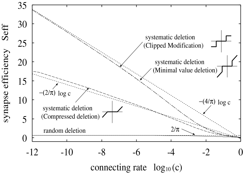
Figure 15: Comparison of the synapse efficiency with the random deletion and that with the systematic deletion at the firing rate $f=0.5$.

IV The memory performance under limited metabolic energy resources

Until the previous section, we have discussed the effect of synaptic pruning by evaluating the synapse efficiency which is the memory capacity normalized by connecting rate $c$. When the connecting rate is $c$, the synapse number per one neuron decreases to $cN$. Therefore, the synapse efficiency means the capacity per the input of one neuron. In the discussion by the synapse efficiency, the synapse number decreases when the connecting rate is small.

In addition to such the fixed neuron number criterion, a fixed synapse number criterion could be discussed. At the synaptic growth stage, it is natural to assume that metabolic energy resources are restricted. When metabolic energy resources are limited, it is also important that the effect of synaptic pruning is discussed under limited synapse number. Chechik et al. discussed the memorized pattern number per one synapse under a fixed synapse number criterion Chechik1998 D They pointed out the existence of an optimal connecting rate under the fixed synapse number criterion and suggested an explanation of synaptic pruning as follows: synaptic pruning following over-growth can improve performance of a network with limited synaptic resources.

The synapse number is $N^{2}$ in the full connected case $c=1$. We consider the larger network with $M(>N)$ neurons. The synapse number in the lager networks with the connecting rate $c$ becomes $cM^{2}$. We can introduce the fixed synapse number criterion by considering a larger network which has $M$ neurons, i.e.,

$$N^{2}=cM^{2},$$ (59)

synapses at the connecting rate $c$. The memorized pattern number per one synapse becomes

$$\frac{p_{c}}{cM^{2}}=\frac{p_{c}}{N^{2}}=\frac{\alpha_{c}}{N}=\frac{\alpha_{c}}{\sqrt{c}M},$$ (60)

where the critical memorized pattern number $p_{c}$ is

$$p_{c}=\alpha_{c}N.$$ (61)

We define the coefficient $\alpha_{c}/\sqrt{c}$ as memory performance. We discuss the effect of synaptic pruning by the memory performance. Under limited metabolic energy resources, the optimal strategy is the maximization of the memory performance. Chechik et al. showed the existence of the optimal connecting rate which maximize memory performance Chechik1998 . The memory performance can be calculated by normalising the capacity, which is given by solving the order-parameter equations, with $\sqrt{c}$. Figure 16 shows the dependence of the memory performance on the connecting rate in three types of pruning. It is confirmed that there are the optimal values which maximized the memory performance by each deletions. The optimal connecting rates of clipped synapse, minimal value deletion, and compressed deletion are $c=0.036,0.038,0.084$, respectively. This interesting fact may imply that the memory performance is improved without heavy pruning. These optimal values agree with the computer simulation results given by Chechik et al Chechik1998 .

Figure 16: Memory performance $\alpha_{c}/\sqrt{c}$ of networks with different number of neurons but the same total number of synapses as a function of the connecting rate $c$ in the case of clipped synapse (the solid line), minimal value deletion (the dotted line), and compressed deletion (the dashed line).

V Conclusion

We have analytically discussed the synapse efficiency, which we regarded as the auto-correlation-type associative memory, to evaluate the effect of the pruning following over-growth. Although Chechik et al. pointed out that the synapse efficiency is increased by the systematic deletion, this is qualitatively obvious and the increase in the synapse efficiency should also be discussed quantitatively. At the limit where the multiplicative synaptic noise is extremely large, storage capacity $\alpha_{c}$ is inversely as the variance of the multiplicative synaptic noise $\Delta_{M}^{2}$. From this result, we analytically obtained that the synapse efficiency in the case of the systematic deletion diverges as $O(|\log c|)$ at the limit where the connecting rate $c$ is extremely small.

On the other hand, it is natural to assume that metabolic energy resources are restricted at the synaptic growth stage. When metabolic energy resources are limited, i.e., synapse number is limited, the optimal connecting rate, which maximize memory performance, exists. These optimal values are in agreement with the results given by Chechik et al Chechik1998 .

In the correlation learning, which can be considered a prototype of any other learning rules, various properties can be analyzed quantitatively. The asymptote of synapse efficiency in the model with another learning rule can be discussed in a similar way. As our future work, we plan to further discuss these properties while taking into account various considerations regarding related physiological knowledge.

ACKNOWLEDGEMENTS

We thank the referee for the helpful comments, especially for the comment concerning the derivation of Appendix C. This work was partially supported by a Grant-in-Aid for Scientific Research on Priority Areas No. 14084212, for Scientific Research (C) No. 14580438, for Encouragement of Young Scientists (B) No. 14780309 and for Encouragement of Young Scientists (B) No. 15700141 from the Ministry of Education, Culture, Sports, Science and Technology of Japan.

Appendix A SCSNA for additive synaptic noise

Derivations of the order-parameter Eqs.(23) -(27) are given here. The SCSNA starts from the fixed-point equations for the dynamics of the $N$-neuron network shown as Eq.(1). The random memory patterns are generated according to the probability distribution of Eq.(2). The syanaptic connections are given by Eq.(4). The asymmetric additive synaptic noise, $\delta_{ij}$ and $\delta_{ji}$ are independently generated according to the probability distribution of Eq.(7). Moreover, we can analyze a more general case, where $\delta_{ij}$ and $\delta_{ji}$ have an arbitary correlation such that

$${\rm Cov}[\delta_{ij},\delta_{ji}]=k_{\delta}\frac{J^{2}}{N(1-a^{2})^{2}}\Delta_{A}^{2},\quad-1\leq k_{\delta}\leq 1.$$ (62)

In this general case, the symmetric and the asymmetric additive synaptic noise correspond to $k_{\delta}=1$ and $k_{\delta}=0$, respectively. Here, we assume the probability distribution of the additive syanptic noise is normal distribution $\delta_{ij}\sim N(0,\frac{J^{2}}{N(1-a^{2})^{2}}\Delta_{A}^{2})$. However, any probability distributions, which have same average and variance, can be discussed by the central limit theorem in the similar way of the following disscussion. Defining the loading rate as $\alpha=p/N$, we can write the local field $h_{i}$ for neuron $i$ as

$$h_{i} \equiv \sum_{j\neq i}^{N}J_{ij}x_{j}$$ (63)

$$= J\sum_{\mu=1}^{\alpha N}(\xi_{i}^{\mu}-a)m_{\mu}+\sum_{j\neq i}^{N}\delta_{ij}x_{j}-J\alpha x_{i},$$

where $m_{\mu}$ is the overlap between the stored pattern $\mbox{\boldmath$\xi$}^{\mu}$ and the equilibrium state $x$ defined by

$$m_{\mu}=\frac{1}{N(1-a^{2})}\sum_{i=1}^{N}(\xi^{\mu}_{i}-a)x_{i}.$$ (64)

The second term including $x_{j}=F(h_{j}+h)$ in Eq.(63) depends on $\delta_{ji}$. The $\delta_{ij}$ dependences of $x_{j}$ are extracted from $x_{j}$,

$$x_{j}=x^{(\delta_{ji})}_{j}+\delta_{ji}x_{i}x^{\prime}{}^{(\delta_{ji})}_{j},$$ (65)

where

$$x^{(\delta_{ji})}_{j} = F(h_{j}-\delta_{ji}x_{i}),$$ (66)

$$x^{\prime}{}^{(\delta_{ji})}_{j} = F^{\prime}(h_{j}-\delta_{ji}x_{i}).$$ (67)

Substituting Eq.(65) into Eq.(63), the local field $h_{i}$ can be expressed as

$$h_{i} = J\sum_{\mu=1}^{\alpha N}(\xi_{i}^{\mu}-a)m_{\mu}+\sum_{j\neq i}^{N}\delta_{ij}x^{(\delta_{ji})}_{j}-J\alpha x_{i}$$ (68)

$$+x_{i}\sum_{j\neq i}^{N}\delta_{ij}\delta_{ji}x^{\prime}{}^{(\delta_{ji})}_{j}.$$

We assume that Eq.(68) and $x_{i}=F(h_{i}+h)$ can be solved by using the effective response function $\tilde{F}(u)$ as,

$$x_{i}=\tilde{F}\biggl{(}J\sum_{\mu=1}^{p}(\xi_{i}^{\mu}-a)m_{\mu}+\sum_{j\neq i}^{N}\delta_{ij}x^{(\delta_{ji})}_{j}\biggr{)}.$$ (69)

Let $\mbox{\boldmath$\xi$}^{1}$ be the target pattern to be retrieved. Therefore, we can assume that $m_{1}=O(1)$ and $m_{\mu}=O(1/\sqrt{N}),\mu>1$. Then we can use the Taylor expansion to obtain

$$m_{\mu} = \frac{1}{N(1-a^{2})}\sum_{i=1}^{N}(\xi_{i}^{\mu}-a)x_{i}^{(\mu)}$$ (70)

$$+\frac{J}{N(1-a^{2})}\sum_{i=1}^{N}(\xi^{\mu}_{i}-a)^{2}m_{\mu}x^{\prime}{}^{(\mu)}_{i}$$

$$= \frac{1}{N(1-a^{2})}\sum_{i=1}^{N}(\xi_{i}^{\mu}-a)x_{i}^{(\mu)}+JUm_{\mu}$$

$$= \frac{1}{N(1-a^{2})(1-JU)}\sum_{i=1}^{N}(\xi_{i}^{\mu}-a)x_{i}^{(\mu)},$$

by substituting Eq.(69) into the overlap defined by Eq.(64), where

$$x^{(\mu)}_{i} = \tilde{F}\biggl{(}J\sum_{\nu\neq\mu}^{\alpha N}(\xi_{i}^{\nu}-a)m_{\nu}+\sum_{j\neq i}^{N}\delta_{ij}x^{(\delta_{ji})}_{j}\biggr{)},$$ (71)

$$x^{\prime}{}^{(\mu)}_{i} = \tilde{F}^{\prime}\biggl{(}J\sum_{\nu\neq\mu}^{\alpha N}(\xi_{i}^{\nu}-a)m_{\nu}+\sum_{j\neq i}^{N}\delta_{ij}x^{(\delta_{ji})}_{j}\biggr{)},$$ (72)

$$U = \frac{1}{N}\sum_{i=1}^{N}x^{\prime}{}^{(\mu)}_{i}.$$ (73)

Equations (68) and (70) give the following expression for the local field:

$$h_{i} = J(\xi^{1}_{i}-a)m_{1}$$ (74)

$$+\alpha\left[\frac{J^{2}}{1-JU}+k_{\delta}\frac{J^{2}}{(1-a^{2})^{2}}\Delta_{A}^{2}\right]Ux_{i}$$

$$+\frac{J}{N(1-a^{2})(1-JU)}\sum_{j\neq i}^{N}\sum_{\mu=2}^{\alpha N}(\xi^{\mu}_{i}-a)(\xi^{\mu}_{j}-a)x_{j}^{(\mu)}$$

$$+\sum_{j\neq i}^{N}\delta_{ij}x^{(\delta_{ji})}_{j}.$$

Note that the second term in Eq.(74) denotes the effective self-coupling term. The third and the last terms are summations of uncorrelated random variables, with mean 0 and variance,

$$\frac{J^{2}}{N^{2}(1-a^{2})^{2}(1-JU)^{2}}$$

$$\quad\times\sum_{j\neq i}^{N}\sum_{\mu=2}^{\alpha N}(\xi_{i}^{\mu}-a)^{2}(\xi_{j}^{\mu}-a)^{2}(x_{j}^{(\mu)})^{2}$$

$$\qquad\qquad=\frac{\alpha J^{2}}{(1-JU)^{2}}q,$$ (75)

$$\sum_{j\neq i}^{N}\delta_{ij}^{2}(x_{j}^{(\delta_{ji})})^{2}=\frac{J^{2}}{(1-a^{2})^{2}}\Delta_{A}^{2}q,$$ (76)

respectively. The cross term of these terms have vanished. Thus, we finally obtain

$$h_{i} = J(\xi^{1}_{i}-a)m_{1}+\sigma z_{i}$$ (77)

$$+\biggl{[}\frac{\alpha J^{2}}{1-JU}+k_{\delta}\frac{J^{2}}{(1-a^{2})^{2}}\Delta_{A}^{2}\biggr{]}Ux_{i}$$

$$\sigma^{2} = \frac{\alpha J^{2}q}{(1-JU)^{2}}+\frac{J^{2}}{(1-a^{2})^{2}}\Delta_{A}^{2}q,$$ (78)

from Eqs.(75) and (76), where $z_{i}\sim N(0,1)$. Equation (26) is given by Eq.(78). Finally, after rewriting $\xi^{1}_{i}\to\xi$, $m_{1}\to m$, $z_{i}\to z$, and $x_{i}\to Y(z;\xi)$, the results of the SCSNA for the additive synaptic noise are summarized by the order-parameter equations of Eqs.(23) -(25) as,

$$m = \frac{1}{1-a^{2}}\int Dz<(\xi-a)Y(z;\xi)>_{\xi},$$

$$q = \int Dz<Y(z;\xi)^{2}>_{\xi},$$

$$U = \frac{1}{\sigma}\int Dz\;z<Y(z;\xi)>_{\xi},$$

where the effective response function $Y(z;\xi)$ becomes

$$Y(z;\xi) = F\biggl{(}J(\xi-a)m+\sigma z+h$$

$$+\biggl{[}\frac{\alpha J^{2}}{1-JU}+k_{\delta}\frac{J^{2}}{(1-a^{2})^{2}}\Delta_{A}^{2}\biggr{]}UY(z;\xi)\biggr{)}.$$

The effective response function of Eq.(27) can be obtained by substituting $k_{\delta}=1$ into Eq.(LABEL:ap:effective_response_function).

Appendix B Equivalence among three types of noise

The multiplicative synaptic noise, the random synaptic deletion, and the nonlinear synapse can be discussed in the similar manner to Appendix A.

B.1 Multiplicative synaptic noise

Derivations of the equivalent noise Eq.(29) is given here. We can also analyze by a similar manner to the analysis of the additive synaptic noise. The syanaptic connections are given by Eq.(8). The asymmetric multiplicative synaptic noise, $\varepsilon_{ij}$ and $\varepsilon_{ji}$ are independently generated according to the probability distribution of Eq.(9). We analyze a more general case, where $\delta_{ij}$ and $\delta_{ji}$ have an arbitary correlation such that

$$\mbox{Cov}[\varepsilon_{ij},\varepsilon_{ji}]=k_{\varepsilon}\Delta_{M}^{2},\quad-1\leq k_{\varepsilon}\leq 1.$$ (80)

In this general case, the symmetric and the asymmetric multiplicative synaptic noise correspond to $k_{\varepsilon}=1$ and $k_{\varepsilon}=0$, respectively. Here, we assume the probability distribution of the multiplicative synaptic noise is normal distribution $\varepsilon_{ij}\sim N(0,\Delta_{M}^{2})$. The local field $h_{i}$ for neuron $i$ becomes

$$h_{i} = \sum_{\mu=1}^{\alpha N}(\xi_{i}^{\mu}-a)m_{\mu}$$ (81)

$$+\frac{1}{N(1-a^{2})}\sum_{\mu=1}^{\alpha N}\sum_{j\neq i}^{N}\varepsilon_{ij}(\xi_{i}^{\mu}-a)(\xi_{j}^{\mu}-a)x_{j}$$

$$-\alpha x_{i},$$

where $m_{\mu}$ is the overlap defined by Eq.(64). The second term including $x_{j}=F(h_{j}+h)$ in Eq.(81) depends on $\varepsilon_{ji}$. The $\varepsilon_{ij}$ dependences and $\xi_{j}^{\mu}$ dependences of $x_{j}$ are extracted from $x_{j}$,

$$x_{j} = x^{(\mu)(\varepsilon_{ji})}_{j}+h_{j}^{\{\mu,\varepsilon_{ji}\}}x^{\prime}{}^{(\mu)(\varepsilon_{ji})}_{j},$$ (82)

$$h_{j}^{\{\mu,\varepsilon_{ji}\}} = (\xi^{\mu}_{j}-a)m_{\mu}$$ (83)

$$+\frac{1}{N(1-a^{2})}\sum_{k\neq j}^{N}\varepsilon_{jk}(\xi_{j}^{\mu}-a)(\xi_{k}^{\mu}-a)x_{k}$$

$$+\frac{\varepsilon_{ji}}{N(1-a^{2})}\sum_{\nu\neq\mu}^{\alpha N}(\xi_{j}^{\nu}-a)(\xi_{i}^{\nu}-a)x_{i}$$

$$+\frac{\varepsilon_{ji}}{N(1-a^{2})}(\xi_{j}^{\mu}-a)(\xi_{i}^{\mu}-a)x_{i},$$

where

$$x^{(\mu)(\varepsilon_{ji})}_{j} = F(h_{j}-h_{j}^{\{\mu,\varepsilon_{ji}\}}),$$ (84)

$$x^{\prime}{}^{(\mu)(\varepsilon_{ji})}_{j} = F^{\prime}(h_{j}-h_{j}^{\{\mu,\varepsilon_{ji}\}}).$$ (85)

We assume that Eq.(81) and $x_{i}=F(h_{i}+h)$ can be solved by using the effective response function $\tilde{F}(u)$ as,

$$x_{i}=\tilde{F}(\sum_{\mu=1}^{p}(\xi_{i}^{\mu}-a)m_{\mu}$$

$$+\frac{1}{N(1-a^{2})}\sum_{\mu=1}^{\alpha N}\sum_{j\neq i}^{N}\varepsilon_{ij}(\xi_{i}^{\mu}-a)(\xi_{j}^{\mu}-a)x^{(\mu)(\varepsilon_{ji})}_{j}).$$

(86)

Let $\mbox{\boldmath$\xi$}^{1}$ be the target pattern. We substitute Eq.(86) into the overlap defined by Eq.(64) and expand the resultant expression by $(\xi_{i}^{\mu}-a)m_{\mu}$ $(\mu>1)$, which has the order of $O(1/\sqrt{N})$. This leads to

$$m_{\mu}=\frac{1}{N(1-a^{2})(1-U)}\sum_{i=1}^{N}(\xi_{i}^{\mu}-a)x_{i}^{(\mu)},$$ (87)

where

$$x^{(\mu)}_{i}=\tilde{F}\biggl{(}\sum_{\nu\neq\mu}^{\alpha N}(\xi_{i}^{\nu}-a)m_{\nu}$$

$$+\frac{1}{N(1-a^{2})}\sum_{\nu\neq\mu}^{\alpha N}\sum_{j\neq i}^{N}\varepsilon_{ij}(\xi_{i}^{\nu}-a)(\xi_{j}^{\nu}-a)x^{(\nu)(\varepsilon_{ji})}_{j}\biggr{)},$$

and $U$ is defined by the similar way of Eq.(73) in the case of the additive synaptic noise. Equations (81),(82) and (87) give

$$h_{i} = (\xi^{1}_{i}-a)m_{1}+\alpha\left[\frac{1}{1-U}+k_{\varepsilon}\Delta_{M}^{2}\right]Ux_{i}$$

$$+\frac{1}{N(1-a^{2})(1-U)}\sum_{j\neq i}^{N}\sum_{\mu=2}^{\alpha N}(\xi^{\mu}_{i}-a)(\xi^{\mu}_{j}-a)x_{j}^{(\mu)}$$

$$+\frac{1}{N(1-a^{2})}\sum_{\mu=1}^{\alpha N}\sum_{j\neq i}^{N}\varepsilon_{ij}(\xi_{i}^{\mu}-a)(\xi_{j}^{\mu}-a)x^{(\mu)(\varepsilon_{ji})}_{j}.$$

The third and last terms can be regarded as the noise terms. The variance of the noise terms becomes

$$\sigma^{2}=\frac{\alpha q}{(1-U)^{2}}+\alpha\Delta_{M}^{2}q.$$ (90)

Thus, after rewriting $\xi_{i}^{1}\to\xi$ and $m_{1}\to m$, we obtain the effective response function:

$$Y(z;\xi) = F\biggl{(}(\xi-a)m+\sigma z+h$$

$$+\alpha\left[\frac{1}{1-U}+k_{\varepsilon}\Delta_{M}^{2}\right]UY(z;\xi)\biggr{)}.$$

Finally, the equivalence between the multiplicative synaptic noise and the additive synaptic noise is obtained as follows,

$$J = 1,$$ (92)

$$\Delta_{A}^{2} = \alpha(1-a^{2})^{2}\Delta_{M}^{2},$$ (93)

$$k_{\delta} = k_{\varepsilon},$$ (94)

by comparing Eqs.(90) and (LABEL:ap:mul.Y.final) to Eqs.(78) and (LABEL:ap:effective_response_function).

B.2 Random deletion

Derivations of the equivalent noise Eq.(30) is given here. The random deletion has similar effects to the multiplicative synaptic noise. Therefore, we analyse by a similar way to the analysis of the multiplicative synaptic noise. The syanaptic connections are given by Eq.(10). The asymmetric cut coefficients are independently generated according to the probability distribution of Eq.(11). We analyze a more general case, where $c_{ij}$ and $c_{ji}$ have an arbitary correlation such that

$$\mbox{Cov}[c_{ij},c_{ji}] = k_{c}\mbox{Var}[c_{ij}],\quad-1\leq k_{c}\leq 1$$ (95)

$$\mbox{Var}[c_{ij}] = \mbox{E}[(c_{ij})^{2}]-(\mbox{E}[c_{ij}])^{2}$$ (96)

$$= c(1-c).$$

In this general case, the symmetric and asymmetric random deletion correspond to $k_{c}=1$ and $k_{c}=0$, respectively. According to a similar analysis of the multiplicative synaptic noise, the local field becomes

$$h_{i} = (\xi^{1}_{i}-a)m_{1}+\alpha\left[\frac{1}{1-U}+\frac{k_{c}(1-c)}{c}\right]Ux_{i}$$ (97)

$$+\frac{1}{N(1-a^{2})(1-U)}\sum_{j\neq i}^{N}\sum_{\mu=2}^{\alpha N}(\xi^{\mu}_{i}-a)(\xi^{\mu}_{j}-a)x_{j}^{(\mu)}$$

$$+\frac{1}{Nc(1-a^{2})}\sum_{\mu=1}^{\alpha N}\sum_{j\neq i}^{N}(c_{ij}-c)$$

$$\qquad\qquad\times(\xi_{i}^{\mu}-a)(\xi_{j}^{\mu}-a)x^{(\mu)(c_{ji})}_{j},$$

where

$$x^{(\mu)(c_{ji})}_{j}=F(h_{j}-h_{j}^{\{\mu,c_{ji}\}}),$$ (98)

$$x^{(\mu)}_{i}=\tilde{F}\biggl{(}\sum_{\nu\neq\mu}^{\alpha N}(\xi_{i}^{\nu}-a)m_{\nu}+\frac{1}{Nc(1-a^{2})}$$

$$\quad\times\sum_{\nu\neq\mu}^{\alpha N}\sum_{j\neq i}^{N}(c_{ij}-c)(\xi_{i}^{\nu}-a)(\xi_{j}^{\nu}-a)x^{(\nu)(c_{ji})}_{j}\biggr{)},$$

(99)

$$h_{j}^{\{\mu,c_{ji}\}}=(\xi^{\mu}_{j}-a)m_{\mu}+\frac{1}{Nc(1-a^{2})}$$

$$\quad\times\sum_{k\neq j}^{N}(c_{jk}-c)(\xi_{j}^{\mu}-a)(\xi_{k}^{\mu}-a)x_{k}$$

$$\quad+\frac{c_{ji}-c}{Nc(1-a^{2})}\sum_{\nu\neq\mu}^{\alpha N}(\xi_{j}^{\nu}-a)(\xi_{i}^{\nu}-a)x_{i}$$

$$\quad+\frac{c_{ji}-c}{Nc(1-a^{2})}(\xi_{j}^{\mu}-a)(\xi_{i}^{\mu}-a)x_{i},$$ (100)

and $U$ is defined by Eq.(73) similarly. The variance of the noise term is given by

$$\sigma^{2}=\frac{\alpha q}{(1-U)^{2}}+\alpha\frac{1-c}{c}q.$$ (101)

Thus, after rewriting $\xi_{i}^{1}\to\xi$ and $m_{1}\to m$, the effective response function becomes

$$Y(z;\xi) = F\biggl{(}(\xi-a)m+\sigma z+h$$

$$+\alpha\left[\frac{1}{1-U}+\frac{k_{c}(1-c)}{c}\right]UY(z;\xi)\biggr{)}.$$

Finally, the equivalence between random deletion and the additive synaptic noise is obtained as follows,

$$J = 1,$$ (103)

$$\Delta_{A}^{2} = \alpha(1-a^{2})^{2}\frac{1-c}{c},$$ (104)

$$k_{\delta} = k_{c},$$ (105)

by comparing Eqs.(101) and (LABEL:ap:random_deletion.Y) to Eqs.(78) and (LABEL:ap:effective_response_function). Substituting Eq.(104) into Eq.(93), we obtain the equivalence of Eq.(30).

B.3 Nonlinear synapse

Derivations of the equivalent noise Eq.(31) is given here. The effect of the nonlinear synapse can be separated into a signal part and a noise part. The noise part can be regarded as the additive synaptic noise.

The systematic deletion of synaptic connections can be achieved by introducing synaptic noise with an appropriate nonlinear function $f(x)$ Sompolinsky1986b . Note that $T_{ij}$ obeys the normal distribution $N(0,1)$ for $p=\alpha N\to\infty$. According to this naive S/N analysis Okada1998 , we can write the connections as

$$J_{ij} = \frac{\sqrt{p}}{N}f(T_{ij})$$ (106)

$$= \frac{J}{N(1-a^{2})}\sum_{\mu=1}^{p}(\xi_{i}^{\mu}-a)(\xi_{j}^{\mu}-a)$$

$$-\biggl{[}\frac{\sqrt{p}}{N}f(T_{ij})-\frac{J}{N(1-a^{2})}\sum_{\mu=1}^{p}(\xi_{i}^{\mu}-a)(\xi_{j}^{\mu}-a)\biggr{]}$$

$$= \frac{\sqrt{p}}{N}\{JT_{ij}-[f(T_{ij})-JT_{ij}]\}.$$

The following derivation suggests that the residual overlap $m_{\mu}$ for the first term in Eq.(106) is enhanced by a factor of $1/(1-JU)$, while any enhancement to the last part is canceled because of the subtraction. It also implies that the last part corresponds to the synaptic noise. For the SCSNA of the nonlinear synapse, we can analyze by a similar manner of the analysis of the additive synaptic noise. We obtain the local field:

$$h_{i} = J(\xi_{i}^{1}-a)m_{1}+\alpha\left[\frac{J^{2}}{1-JU}+(\tilde{J^{2}}-J^{2})\right]Ux_{i}$$

$$+\frac{\sqrt{p}}{N}\sum_{j\neq i}\left[f(T_{ij})-JT_{ij}\right]x^{(T_{ji})}_{j}$$

$$+\frac{J}{N(1-a^{2})(1-JU)}\sum_{\mu=2}^{p}\sum_{j\neq i}^{N}(\xi_{i}^{\mu}-a)(\xi_{j}^{\mu}-a)x_{j}^{(\mu)},$$

where

$$x^{(\mu)}_{i} = \tilde{F}\biggl{(}J\sum_{\nu\neq\mu}^{p}(\xi_{i}^{\nu}-a)m_{\nu}$$ (108)

$$+\frac{\sqrt{p}}{N}\sum_{j\neq i}^{N}[f(T^{(\mu)}_{ij})-JT^{(\mu)}_{ij}]x^{(T_{ji})}_{j}\biggr{)},$$

$$x^{(T_{ji})}_{j} = F\biggl{(}h_{j}-\frac{\sqrt{p}}{N}[f(T_{ji})-JT_{ji}]x_{i})\biggr{)},$$ (109)

$$T^{(\mu)}_{ij} = \frac{1}{\sqrt{p}(1-a^{2})}\sum_{\nu\neq\mu}^{p}(\xi_{i}^{\nu}-a)(\xi_{j}^{\nu}-a),$$ (110)

and $U$ is defined by Eq.(73) similarly. The variance of the noise term is given by

$$\sigma^{2}=\frac{\alpha J^{2}q}{(1-JU)^{2}}q+\alpha(\tilde{J^{2}}-J^{2}).$$ (111)

Thus, after rewriting $\xi_{i}^{1}\to\xi$ and $m_{1}\to m$, The effective response function becomes

$$Y(z;\xi) = F\biggl{(}J(\xi-a)m+\sigma z+h$$

$$+\alpha\left[\frac{J^{2}}{1-JU}+(\tilde{J^{2}}-J^{2})\right]UY(z;\xi)\biggr{)}.$$

Finally, the equivalence between the nonlinear synapse and the additive synaptic noise is obtained as follows,

$$\Delta_{A}^{2} = \alpha(1-a^{2})^{2}\biggl{(}\frac{\tilde{J^{2}}}{J^{2}}-1\biggr{)},$$ (113)

$$J = \int Dx\;xf(x)$$ (114)

$$\tilde{J^{2}} = \int Dxf(x)^{2}$$ (115)

by comparing Eqs.(111) and (LABEL:ap:nonlinear.Y) to Eqs.(78) and (LABEL:ap:effective_response_function). Substituting Eq.(113) into Eq.(93), we obtain the equivalence of Eq.(31).

Appendix C Asymptote for large multiplicative synaptic noise

Derivations of the asymptote of storage capacity in a large multiplicative synaptic noise $\Delta_{M}$ is given here.

In Eqs.(23) -(25), let $a=0$, $J=1$, and $F(x)=\mbox{sgn}(x)$, the order-parameter equations become

$$m = \mbox{erf}\biggl{(}\frac{m}{\sqrt{2}\sigma}\biggr{)},$$ (116)

$$q = 1,$$ (117)

$$U = \frac{1}{\sigma}\sqrt{\frac{2}{\pi}}\exp\biggl{(}-\frac{m^{2}}{2\sigma^{2}}\biggr{)},$$ (118)

the threshold becomes $h=0$, the effective response function of Eq.(27) and the variance of the noise become

$$Y(z;\xi) = {\rm sgn}(\xi m+\sigma z),$$ (119)

$$\sigma^{2} = \frac{\alpha}{(1-U)^{2}}+\Delta_{A}^{2},$$ (120)

respectively, where the error function ${\rm erf}(x)$ is defined as

$${\rm erf}(x)=\frac{2}{\sqrt{\pi}}\int_{0}^{x}e^{-u^{2}}du.$$ (121)

The slope of the r.h.s. of Eq.(116) is given by

$$\frac{d}{dm}\mbox{erf}\biggl{(}\frac{m}{\sqrt{2}\sigma}\biggr{)}=\frac{1}{\sigma}\sqrt{\frac{2}{\pi}}\exp\biggl{(}-\frac{m^{2}}{2\sigma^{2}}\biggr{)}.$$ (122)

Equation (116) has nontrivial solutions $m\neq 0$ within the range where the slope of the r.h.s. of Eq.(122) at $m=0$ is greater than 1. Therefore, the critical value of the noise $\sigma_{c}^{2}$ is given by

$$\sigma_{c}^{2}=2/\pi.$$ (123)

This shows that a retrieval phase exists only for $\sigma<\sigma_{c}$. We define the parameter $\tau(<1)$ defined as

$$\tau=\frac{\sigma}{\sigma_{c}},$$ (124)

to solve for $m$ as a function of $\sigma$ in the vicinity of this critical value $\sigma_{c}$. The critical value of the additive synaptic noise is discussed in the case of $\tau\simeq 1$. The overlap $m$ shows the first order phase transition when $\Delta_{A}$ is small, but it is regarded as the second order phase transition at large $\Delta_{A}$ region. The overlap becomes $m\ll 1$ when $\tau\simeq 1$ and $\Delta_{A}$ is sufficiently large, therefore the nontrivial solution of $m$ is given as

$$m\simeq\frac{m}{\tau}-\frac{m^{3}}{6\sigma^{2}\tau}+O(m^{4})=\sigma_{c}\tau\sqrt{6(1-\tau)},$$ (125)

by Taylor expansion including terms up to the third order. Substituting Eq.(125) into Eq.(118), $U$ becomes

$$U\simeq\frac{1}{\tau}\biggl{(}1-\frac{m^{2}}{2\sigma^{2}}\biggr{)}+O(m^{4})=3-2\tau^{-1}.$$ (126)

From Eq.(29), the variance of the multiplicative synaptic noise $\Delta_{M}^{2}$ is related to the variance of the additive synaptic noise $\Delta_{A}^{2}$ as

$$\Delta_{A}^{2}=\alpha\Delta_{M}^{2},$$ (127)

when bias $a=0$. Therefore, substituting Eqs.(126) and (127) into Eq.(120), the variance of the noise $\sigma$ is given as

$$\sigma^{2}=\frac{\alpha\tau^{2}}{4(1-\tau)^{2}}+\alpha\Delta_{M}^{2}.$$ (128)

The loading rate $\alpha$ becomes

$$\alpha=\frac{8}{\pi}\cdot\frac{\tau^{2}(1-\tau)^{2}}{\tau^{2}+4\Delta_{M}^{2}(1-\tau^{2})}.$$ (129)

When the overlap is small enough, i.e., $m\ll 1$, the order-parameter equations of Eqs. (116)-(120) reduce to Eq. (129). Solving Eq.(129) for the fixed value of $\alpha$ and $\Delta_{M}$, we obtain the parameter $\tau$. Substituting $\tau$ into Eq. (125), we can obtain the overlap $m$ for given $\alpha$ and $\Delta_{M}$. It is easily confirmed that the $\tau$ increases with $\alpha$ for the fixed value of $\Delta_{M}$. This means that the maximal value of $\tau$ which holds Eq. (129) corresponds to the maximum value of $\alpha$, that is storage capacity $\alpha_{c}$. The critical value $\tau_{c}$ is equal to the value which maximizes the loading rate of Eq.(129) and becomes

$$\tau_{c}=\frac{(2\Delta_{M})^{2/3}}{1+(2\Delta_{M})^{2/3}}\simeq 1-(2\Delta_{M})^{-2/3},$$ (130)

in a large $\Delta_{M}$ limit. Therefore, substituting Eq. (130) into Eq.(129), we obtain Eq.(34) as follows:

$$\alpha_{c}=\frac{2}{\pi\Delta_{M}^{2}}.$$ (131)

References

- (1) P. R. Huttenlocker, Brain Res. 163 195 (1979).
- (2) P. R. Huttenlocker, C. De Courten, L. J. Garey, and H. Van der Loos, Neurosci. lett. 33, 247 (1982).
- (3) J. P. Bourgeois and P. Rakic, J. Neurosci. 13, 2801 (1993).
- (4) J. Takacs and J. Hamori, J. of Neurosci. Research 38, 515 (1994).
- (5) G. M. Innocenti, Trends Neurosci. 18, 397 (1995).
- (6) M. F. Eckenhoff and P. Rakic, Developmental Brain Research 64, 129 (1991).
- (7) P. Rakic, J. P. Bourgeois, and P. S. Goldman-Rakic, Progress in Brain Research 102, 227 (1994).
- (8) M. P. Stryker, J. of Neurosci. 6, 2117 (1986).
- (9) A. W. Roe, S. L. Pallas, J. O. Hahm, and Sur, Science 250, 818 (1990).
- (10) J. R. Wolff, R. Laskawi, W. B. Spatz, and M. Missler, Behavioural Brain Research 66, 13 (1995).
- (11) H. Yanai and S. Amari, IEEE Trans. on Neural Netw. 7, 803 (1996).
- (12) D. J. Amit, N. Brunel, and M. V. Tsodyks, Journal of Neuroscience 14, 6435 (1994).
- (13) M. Griniasty, M. V. Tsodyks, and D. J. Amit, Neural Computation 5, 1 (1993).
- (14) H. Sompolinsky, Phys. Rev. A 34, 2571 (1986).
- (15) G. Chechik, I. Meilijson, and E. Ruppin, Neural Computation 10, 1759 (1998).
- (16) M. Okada, T. Fukai, and M. Shiino, Phys. Rev. E 57, 2095 (1998).
- (17) D. J. Amit, H. Gutfreund, and H. Sompolinsky, Phys. Rev. A 35, 2293 (1987).
- (18) S. Amari, Neural Networks 2, 451 (1989).
- (19) I. Meilijson and E. Ruppin, Biol. Cybern. 74, 479 (1996).
- (20) M. Okada, Neural Netw. 9, 1429 (1996).
- (21) M. Shiino and T. Fukai, J. Phys. A 25, L375 (1992).
- (22) M. Shiino and T. Fukai, Phys. Rev. E 48, 867 (1993).
- (23) M. Okada, Neural Netw. 8, 833 (1995).
- (24) K. Mimura, M. Okada, and K. Kurata, IEICE Trans. Information and systems E81-D 8, 928 (1998).
- (25) K. Mimura, M. Okada, and K. Kurata, IEICE Trans. Information and systems E81-D 11, 1298 (1998).
- (26) T. Kimoto, M. Okada, Biol. Cybern. 85, 319 (2001).
- (27) H.Sompolinsky, in J.L.van Hemmen, I.Morgenstern (eds.), Heidelberg Colloquium on Glassy Dynamics, 485, Springer-Verlag (1987).
- (28) M. V. Tsodyks, M. V. Feigelman, Europhys. Lett. 6, 101 (1988).
- (29) J. Buhmann, R. Divko, and K. Schulten, Phys. Rev. A 39, 2689 (1989).
- (30) C. J. Perez-Vincente and D. J. Amit, J. Phys. A 22, 559 (1989).