Paramagnetic State of Degenerate Double Exchange Model:
a Non-Local CPA Approach

Abstract

The off-diagonal disorder caused by random spin orientations in the paramagnetic (PM) state of the double exchange (DE) model is described by using the coherent-potential-approximation (CPA), which is combined with the variational mean-field approach for the Curie temperature ($T_{C}$). Our CPA approach is essentially non-local and based on the perturbation theory expansion for the $T$-matrix with respect to the fluctuations of hoppings from the ”mean values” specified by matrix elements of the self energy, so that in the first order it becomes identical to the DE theory by de Gennes. The second-order effects, considered in the present work, can be viewed as an extension of this theory. They are not negligible, and lead to a substantial reduction of $T_{C}$ in the one-orbital case. Even more dramatic changes are expected in the case of orbital degeneracy, when each site of the cubic lattice is represented by two $e_{g}$ orbitals, which also specify the form of interatomic transfer integrals. Particularly, the existence of two Van Hove singularities in the spectrum of degenerate DE model (one of which is expected near the Fermi level in the 30%-doped LaMnO₃) may lead to the branching of CPA solutions, when the Green function and the self energy become double-valued functions in certain region of the complex plane. Such a behavior can be interpreted as an intrinsic inhomogeneity of the PM state, which consists of two phases characterized by different electronic densities. The phase separation occurs below certain transition temperature, $T_{P}$, and naturally explains the appearance of several magnetic transition points, which are frequently seen in manganites. We discuss possible implications of our theory to the experimental situation in manganites, as well as possible extensions which needs to be done in order to clarify its credibility.

I Introduction

The nature of paramagnetic (PM) state in perovskite manganese oxides (the manganites) is one of the fundamental questions, the answer to which is directly related with understanding of the phenomenon of colossal magnetoresistance.

There is no doubts that any theoretical model for manganites should include (at least, as one of the main ingredients) the double exchange (DE) physics, which enforces the atomic Hund’s rule and penalizes the hoppings of polarized $e_{g}$ electrons to the sites with the opposite direction of the localized $t_{2g}$ spins.[1, 2, 3] If the spins are treated classically, the corresponding Hamiltonian is given, in the local coordinate frame specified by the directions ${\bf e_{i}}$$=$$(\cos\phi_{\bf i}\sin\theta_{\bf i},\sin\phi_{\bf i}\sin\theta_{\bf i},\cos\theta_{\bf i})$ of the spin magnetic moments, by[4]

$${\cal H}_{\bf ij}=-\xi_{\bf ij}t_{\bf ij},$$ (1)

where $t_{\bf ij}$ are the bare transfer integrals between sites ${\bf i}$ and ${\bf j}$ (which can be either scalars or $2$$\times$$2$ matrices depending on how the orbital degeneracy of the $e_{g}$ states is treated in the model), and $\xi_{\bf ij}$$=$$\cos\frac{\theta_{\bf i}}{2}\cos\frac{\theta_{\bf j}}{2}$$+$$\sin\frac{\theta_{\bf i}}{2}\sin\frac{\theta_{\bf j}}{2}e^{-i(\phi_{\bf i}-\phi_{\bf j})}$ describes their modulations caused by the deviation from the ferromagnetic (FM) alignment in the pair ${\bf i}$-${\bf j}$.

The form of Hamiltonian (1) implies that the spin magnetic moments are saturated (due to the strong Hund’s rule coupling) and the spin disorder corresponding to the PM state is in fact an orientational spin disorder. Despite an apparent simplicity of the DE Hamiltonian (1), the description of this orientational spin disorder is not an easy task and so far there were only few theoretical model, which were based on rather severe (and presumably unsatisfactory) approximations.

The first one was proposed by de Gennes more than forty years ago.[3] In his theory, all $\xi_{\bf ij}$ are replaced by an averaged value $\overline{\xi}$, so that the spin disorder enters the model only as a renormalization (narrowing) of the $e_{g}$-bandwidth. The effect is not particularly strong and the fully disordered PM state corresponds to $\overline{\xi}$$=$$\frac{2}{3}$. A generalization of this theory to the case of quantum spins was given by Kubo and Ohata.[5] The same idea was exploited recently in a number of theories aiming to study the behavior of orbital degrees of freedom at elevated temperature,[6] but based on the same kind of simplifications for the spin disorder and its effects on the kinetic energy.

Another direction, which features more recent activity, is the single-site dynamical mean-field theory (DMFT, see Ref. [7] for a review) for the FM Kondo lattice model.[8, 9] The model itself can be viewed as a prototype of the DE Hamiltonian (1) before projecting out the minority-spin states in the local coordinate frame.[4] If the localized $t_{2g}$ spins are treated classically (that is typically the case), this method is similar to the disordered local moment approach proposed by Gyorffy et al.,[10] and based on the coherent-potential-approximation (CPA) for the electronic structure of the disordered state.[11]

Now it is almost generally accepted that both approaches are inadequate as they fail to explain not even all, but a certain number of observations in manganites of a principal character such as the absolute value and the doping dependence of the Curie temperature ($T_{C}$),[12] the insulating behavior above $T_{C}$,[13] and a rich magnetic phase diagram along the temperature axis, which typically show a number of magnetic phase transitions[14] and the phase coexistence[15, 16, 17] in certain temperature interval. Therefore, it is clear that the theory must be revised.

Then, there are two possible ways to precede. One is to modernize the model itself by including additional ingredients such as the Jahn-Teller distortion,[18] the Coulomb correlations,[6, 19] and the disorder effects caused by the chemical substitution.[20] Another possibility is to stick to the basic concept of the DE physics and try to formulate a more advanced theory of the spin disorder described by the Hamiltonian (1), which would go beyond the simple scaling theory by de Gennes[3] as well as the single-site approximation inherent to DMFT.[8, 9]

An attention to the second direction was drawn recently by Varma.[21] The main challenge to the theoretical description of the orientational spin disorder in the DE systems comes from the fact that it enters the Hamiltonian (1) as an off-diagonal disorder of interatomic transfer integrals, which presents a serious and not well investigated problem. In the present work we try to investigate some possibilities along this line by employing a non-local CPA approach.

What do we expect?

1. It was realized very recently that many aspects of seemingly complicated low-temperature behavior of the doped manganites (the rich magnetic phase diagram, optical properties, etc.) can be understood from the viewpoint of DE physics, if the latter is considered in the combination with the realistic electronic structure for the itinerant $e_{g}$ electrons and takes into account the strong dependence of this electronic structure on the magnetic ordering (see, e.g., Ref. [22] and references therein). If this scenario is correct and can be extended to the high-temperature regime (that is still a big question), there should be something peculiar in the electronic structure of the disordered PM state, which can be linked to the unique properties of manganites. In order to gain insight into this problem, let us start with the DE picture by de Gennes, and consider it in the combination with the correct form of the transfer integrals between two $e_{g}$ orbitals on the cubic lattice.[23] Then, the properties of the PM state should be directly related with details of the electronic structure of the FM state, which is shown in Fig. 1 and connected with the PM electronic structure by the scaling transformation. This electronic structure is indeed very peculiar because of two Van Hove singularities at the $(\pi,\pi,0)$ and $(0,\pi,0)$ points of the Brillouin zone, which are responsible for two kinks of density of states at $\pm$$1$. It is also interesting to note that the first singularity appears near the Fermi surface when the hole concentration is close to $0.3$, i.e. in the most interesting regime from the viewpoint of colossal magnetoresistance.[24] Such a behavior was discussed by Dzero, Gor’kov and Kresin.[25] They also argued that this singularity can contribute to the $T^{3/2}$ dependence of the specific heat in the FM state. If so, what is the possible role of these singularities in the case of the spin disorder? Note that apart from the single-site approximation, all recent DMFT calculations[8, 9] employed a model semi-circular density of states, and therefore could not address this problem.

2. There are many anticipations in the literature that there is some hidden degree of freedom which controls the properties of perovskite manganites. A typical example is the picture of orbital disorder proposed in Ref. [19] in connection with the anomalous behavior of the optical conductivity in the FM state of perovskite manganites. According to this picture, the large on-site Coulomb interaction gives rise to the orbital polarization at each site of the system. The local orbital polarizations remain even in the cubic FM phase, but without the long-range ordering. In the present work we will show that, in principle, by considering non-local effects in the framework of pure DE model, one may have an alternative scenario, when there is a certain degree of freedom which does control the properties of manganites. However, contrary to the orbital polarization, this parameter is essentially non-local and attached to the bond of the DE system rather than to the site.

3. There were many debated about the phase separation in perovskite manganites,[26, 27] and according to some scenarios this effect plays an important role also at elevated temperatures, being actually the main trigger behind phenomenon of the colossal magnetoresistance.[20] The problem was intensively studied numerically, using the Monte Carlo techniques.[20, 27] If this is indeed the case, what does it mean on the language of analytical solutions of the DE model (or its refinements)? Presumably, the only possibility to have two (and more) phases at the same time is to admit that the self energy (and the Green function) of the model can be a multi-valued function in certain region of the complex plane. Such a behavior of non-linear CPA equations was considered as one of the main troublemakers in the past,[28, 29] but may have some physical explanation in the light of newly proposed ideas of phase separation.

The rest of the paper is organized as follows. In Sec. II we briefly review the main ideas of the variational mean-field approach. In Sec. III we describe general ideas of the non-local CPA to the problem of orientational spin disorder in the DE systems. In Sec. IV we consider the CPA solution for the PM phase of the one-orbital model and evaluate the Curie temperature. We will argue that two seemingly different approaches to the problem of spin disorder in the DE model, one of which was proposed by de Gennes[3] and the other one is based on the DMFT[8, 9], have a common basis and can be regarded as CPA-type approaches, but supplemented with different types of approximations. In Sec. V we consider more realistic two-orbital case for the $e_{g}$ electrons and argue that it is qualitatively different from the behavior of one-orbital model. Particularly, the CPA self-energy becomes the double-valued function in certain region of the complex plane, that can be related with an intrinsic inhomogeneity of the PM state of the DE model. In Sec. VI we summarize the main results of our work, discuss possible connections with the experimental behavior of perovskite manganites as well as possible extensions.

II Calculation of Thermal Averages

In order to proceed with the finite temperature description of the DE systems we adopt the variational mean-field approach.[3, 5, 30] Namely, we assume that the thermal (or orientational) average of any physical quantity is given in terms of the single spin orientation distribution function, which depends only on the angle between the local spin and an effective molecular field $\lambda$,

$$p_{\bf i}({\bf e}_{\bf i})\propto\exp\left(\mbox{\boldmath$\lambda$}\cdot{\bf e_{i}}\right),$$ (2)

while all correlations between different spins are neglected.[31] In the case of PM-FM transition, the effective field can be chosen as $\lambda$$=$$(0,0,\lambda)$.

The first complication comes from the fact that the DE Hamiltonian (1) is formulated in the local coordinate frame, in which the spin quantization axes at different sites are specified by the different direction $\{{\bf e_{i}}\}$. Therefore, we should clarify the meaning of orientational averaging in the local coordinate frame.[32] From our point of view, it is logical that in order to calculate the thermal averages associated with an arbitrary chosen site ${\bf 0}$, the global coordinate frame should be specified by the direction ${\bf e_{0}}$$=$$(\cos\phi_{\bf 0}\sin\theta_{\bf 0},\sin\phi_{\bf 0}\sin\theta_{\bf 0},\cos\theta_{\bf 0})$, so that at each instant the spin moment at the site ${\bf 0}$ is aligned along the $z$-direction. The averaging over all possible directions ${\bf e_{0}}$ of the global coordinate frame in the molecular field $\lambda$ can be performed as the second step.

Then, corresponding distribution function at the site ${\bf 0}$ is given by Eq. (2). The distribution functions at other sites can be constructed as follows. The transformation to the coordinate frame associated with the site ${\bf 0}$ is given by the matrix:

$$\widehat{R}=\left(\begin{array}[]{ccc}\cos^{2}\phi_{\bf 0}(\cos\theta_{\bf 0}-1)+1&\sin\phi_{\bf 0}\cos\phi_{\bf 0}(\cos\theta_{\bf 0}-1)&-\cos\phi_{\bf 0}\sin\theta_{\bf 0}\\ \sin\phi_{\bf 0}\cos\phi_{\bf 0}(\cos\theta_{\bf 0}-1)&\sin^{2}\phi_{\bf 0}(\cos\theta_{\bf 0}-1)+1&-\sin\phi_{\bf 0}\sin\theta_{\bf 0}\\ \cos\phi_{\bf 0}\sin\theta_{\bf 0}&\sin\phi_{\bf 0}\sin\theta_{\bf 0}&\cos\theta_{\bf 0}\\ \end{array}\right).$$

In the new coordinates, the ${\bf i}$-th moment has the direction ${\bf e}^{\prime}_{\bf i}$$=$$\widehat{R}{\bf e}_{\bf i}$$\equiv$$(\cos\phi^{\prime}_{\bf i}\sin\theta^{\prime}_{\bf i},\sin\phi^{\prime}_{\bf i}\sin\theta^{\prime}_{\bf i},\cos\theta^{\prime}_{\bf i})$, and the effective field becomes $\mbox{\boldmath$\lambda$}^{\prime}$$=$$\widehat{R}\mbox{\boldmath$\lambda$}$$=$$(-\cos\phi_{\bf 0}\sin\theta_{\bf 0},-\sin\phi_{\bf 0}\sin\theta_{\bf 0},\cos\theta_{\bf 0})\lambda$.

Obviously, while $\mbox{\boldmath$\lambda$}^{\prime}$ and ${\bf e}^{\prime}_{\bf i}$ depend on $\theta_{\bf 0}$ and $\phi_{\bf 0}$, the new distribution function $p_{\bf i}({\bf e}^{\prime}_{\bf i})$$\propto$$\exp(\mbox{\boldmath$\lambda$}^{\prime}\cdot{\bf e}^{\prime}_{\bf i})$ – does not, and up to this stage the transformation to the new coordinate frame was only the change of the notations. In order to obtain the total distribution function $P_{\bf i}({\bf e}^{\prime}_{\bf i})$ for ${\bf i}$$\neq$$0$, formulated in the local coordinates of the site ${\bf 0}$ and taking into account the motion of ${\bf e_{0}}$ in the molecular field $\lambda$, $p_{\bf i}({\bf e}^{\prime}_{\bf i})$ should be averaged over ${\bf e_{0}}$ with the weight $p_{\bf 0}({\bf e}_{\bf 0})$:

$$P_{\bf i}({\bf e}^{\prime}_{\bf i},\lambda)=\frac{1}{\nu}\int d\mbox{\boldmath$\Omega$}_{\bf 0}\exp\left(\mbox{\boldmath$\lambda$}^{\prime}\cdot{\bf e}^{\prime}_{\bf i}+\mbox{\boldmath$\lambda$}\cdot{\bf e}_{\bf 0}\right).$$ (3)

The normalization constant $\nu$ is obtained from the condition:

$$\int d\mbox{\boldmath$\Omega$}^{\prime}_{\bf i}P_{\bf i}({\bf e}^{\prime}_{\bf i},\lambda)=1.$$

The form of Eq. (3) implies that the directions of magnetic moments are not correlated (in the spirit of the mean-field approach) and the averaging over ${\bf e}_{\bf 0}$ can be performed independently for different sites of the system. For the analysis the PM state and the magnetic transition temperature, it is sufficient to consider the small-$\lambda$ limit. Then, Eq. (3) becomes:

$$P_{\bf i}({\bf e}^{\prime}_{\bf i},\lambda)\simeq\frac{1}{4\pi}\left(1+\frac{1}{3}\cos\theta^{\prime}_{\bf i}\lambda^{2}\right).$$ (4)

The thermal average of the function $F({\bf e}^{\prime}_{\bf i})$, formulated in the coordinate frame of the site ${\bf 0}$ and taking into account the motion of both ${\bf e_{0}}$ and ${\bf e_{i}}$, is given by

$$\overline{F}(\lambda)=\int d\mbox{\boldmath$\Omega$}^{\prime}_{\bf i}P_{\bf i}({\bf e}^{\prime}_{\bf i},\lambda)F({\bf e}^{\prime}_{\bf i}).$$

The spin entropy can be computed in terms of the molecular field $\lambda$ as:[3]

$$-TS(\lambda)=k_{B}T\int d\mbox{\boldmath$\Omega$}^{\prime}_{\bf i}P_{\bf i}({\bf e}^{\prime}_{\bf i},\lambda)\ln P_{\bf i}({\bf e}^{\prime}_{\bf i},\lambda).$$

In the second order of $\lambda$ this yields (both for ${\bf i}$$=$$0$ and ${\bf i}$$\neq$$0$):

$$-TS(\lambda)\simeq\frac{k_{B}T}{6}\lambda^{2}.$$ (5)

Then, the free energy of the DE model is given by[3, 30]

$${\cal F}(T,\lambda)=E_{D}(T,\lambda)-TS(\lambda),$$ (6)

where $E_{D}(T,\lambda)$ is the electron free energy (or the double exchange energy):

$$E_{D}(T,\lambda)=-\int_{-\infty}^{+\infty}dzf_{T}(z-\mu)\overline{n}(z,\lambda),$$ (7)

calculated in terms of the (orientationally averaged) integrated density of states $\overline{n}(z,\lambda)$. $f_{T}(z$$-$$\mu)$$=$$[\exp(\frac{z-\mu}{k_{B}T})$$+$$1]^{-1}$ is the Fermi-Dirac function ($\mu$ being the chemical potential).

The best approximation for the molecular field $\lambda$ is that which minimizes the free energy (6). Assuming that the transition to the FM state is continuous (of the second order),[33] $T_{C}$ can be found from equation:

$$\left.\frac{\partial^{2}{\cal F}(T_{C},\lambda)}{\partial\lambda^{2}}\right|_{\lambda=0}=0.$$ (8)

In practice, the derivative $\partial^{2}E_{D}(T,\lambda)/\partial\lambda^{2}$ near $\lambda$$=$$0$ can be calculated using the variational properties of $\overline{n}(z,\lambda)$ in CPA and the Lloyd formula.[34, 35]

III Non-Local CPA for the Double Exchange Model

In this section we discuss some general aspects of the non-local CPA to the problem of orientational spin disorder in the DE model specified by the Hamiltonian (1). We attempt to describe the disordered system in an average by introducing an effective energy-dependent Hamiltonian,

$$\overline{\cal H}_{\bf ij}(z)=\Sigma_{\bf ii}(z)\delta_{\bf ij}-\Sigma_{\bf ij}(z)(1-\delta_{\bf ij}),$$ (9)

where $\Sigma_{\bf ij}$ is the non-local part of the self energy, which is restricted by the nearest neighbors; and $\Sigma_{\bf ii}$ is the local (site-diagonal) part. The non-local formulation of CPA is essential because in the low-temperature limit $\overline{\cal H}_{\bf ij}$ should be replaced by the conventional kinetic term in which $\Sigma_{\bf ij}$ plays a role of the bare transfer integral $t_{\bf ij}$. Therefore, $\Sigma_{\bf ij}$ cannot be omitted. On the other hand, $\Sigma_{\bf ii}$ will be needed in order to formulate a closed system of CPA equations.

We require the effective Hamiltonian (9) to preserve the cubic symmetry of the system and be translationally invariant. The first requirement has a different form depending on the degeneracy of the problem and the symmetry properties of basis orbitals, and will be considered separately for the one-orbital and degenerate DE models. In any case, using the symmetry properties, all matrix elements of the self energy $\{\Sigma_{\bf ii},\Sigma_{\bf ij}\}$ on the cubic lattice can be expressed through $\{\Sigma_{\bf 00},\Sigma_{\bf 01}\}$ for one of the dimers (for example, ${\bf 0}$-${\bf 1}$ in Fig. 2). Then, the Hamiltonian (9) can be Fourier transformed to the reciprocal space, $\overline{\cal H}_{\bf q}(z)$$=$$\sum_{\bf j}e^{-i{\bf q}\cdot({\bf R_{i}}-{\bf R_{j}})}\overline{\cal H}_{\bf ij}(z)$, and the first equation for the orientationally averaged Green function can be written as

$$\overline{G}_{\bf ij}(z)=\frac{1}{\Omega_{\rm BZ}}\int d{\bf q}e^{i{\bf q}\cdot({\bf R_{i}}-{\bf R_{j}})}\left[z-\overline{\cal H}_{\bf q}(z)\right]^{-1},$$ (10)

where the integration goes over the first Brillouin zone with the volume $\Omega_{\rm BZ}$.

Unfortunately, the non-local form of the Hamiltonian (9) in the combination with the translational invariance do not necessarily guaranty the fulfillment of causality principle, that is the single-particle Green function should be analytic in the upper half of complex energy plane and satisfy a certain number of physical requirements.[28, 29, 36, 37, 38] This is still a largely unresolved problem, despite numerous efforts over decades. We do not have a general solution to it either. What we try to do here is simply to investigate the behavior of this particular model and try to answer the question whether it is physical or not. Note also that neither dynamical cluster approximation[37] nor cellular DMFT method[38], for which the causality can be rigorously proven, can be easily applied to the problem of off-diagonal disorder.

The calculations near Van Hove singularities in the case of degenerate DE model requires very accurate integration in the reciprocal space. In the present work we used the mesh consisting of 374660 nonequivalent ${\bf q}$-points and corresponding to $258$$\times$$258$$\times$$258$ divisions of the reciprocal lattice vectors.

In order to formulate the CPA equations we consider only site-diagonal and nearest-neighbor elements of $\overline{G}_{\bf ij}$. Again, using the symmetry properties they can be expressed through $\{\overline{G}_{\bf 00},\overline{G}_{\bf 01}\}$. In addition, there is a simple relation between $\overline{G}_{\bf 00}$ and $\overline{G}_{\bf 01}$ for given $\Sigma_{\bf 00}$ and $\Sigma_{\bf 01}$:

$$\overline{G}_{\bf 00}(z)\left[z-\Sigma_{\bf 00}(z)\right]+\sum_{\bf i}\overline{G}_{\bf 0i}(z)\Sigma_{\bf i0}(z)=1,$$ (11)

which follows from the definition of the Green function (10) and the Hamiltonian (9).[39] Using this identity, some matrix elements of the Green function can be easily excluded from CPA equations.

In order to obtain the closed system of CPA equations which connects $\{\Sigma_{\bf 00},\Sigma_{\bf 01}\}$ with $\{\overline{G}_{\bf 00},\overline{G}_{\bf 01}\}$ we construct the $T$-matrix:[34]

$$\widehat{T}(z)=\left[\widehat{\cal H}-\widehat{\overline{\cal H}}(z)\right]\left\{\widehat{1}-\widehat{\overline{G}}(z)\left[\widehat{\cal H}-\widehat{\overline{\cal H}}(z)\right]\right\}^{-1},$$ (12)

and require the average of scattering due to the fluctuations $\Delta\widehat{\cal H}$$=$$\widehat{\cal H}$$-$$\widehat{\overline{\cal H}}$ to vanish on every site and every bond of the system, i.e.:[11, 34]

$$\overline{T}_{\bf 00}(z)=\overline{T}_{\bf 01}(z)=0.$$ (13)

The hat-symbols in Eq. (12) means that all the quantities are infinite matrices in the real space and the matrix multiplications imply also summation over the intermediate sites. Note that our approach is different from the so-called cluster-CPA[28, 29, 36, 40] because the matrix operations in Eq. (12) are not confined within a finite cluster (the dimer, in our case). We believe that our approach is more logical and more consistent with the requirements of the cubic symmetry and the translational invariance of the system, because all dimers are equivalent and should equally contribute to the averaged $T$-matrix. This equivalence is artificially broken in the cluster-CPA approach, which takes into account the contributions of only those atoms which are confined within the cluster. However, our approach also causes some additional difficulties, because the non-local fluctuations $\Delta\widehat{\cal H}$ tend to couple an infinite number of sites in Eq. (12). Therefore, for the practical purposes we restrict ourselves by the perturbation theory expansion up to the second order of $\Delta\widehat{\cal H}$:

$$\widehat{T}(z)\simeq\left[\widehat{\cal H}-\widehat{\overline{\cal H}}(z)\right]+\left[\widehat{\cal H}-\widehat{\overline{\cal H}}(z)\right]\widehat{\overline{G}}(z)\left[\widehat{\cal H}-\widehat{\overline{\cal H}}(z)\right].$$ (14)

As we will show, the first term in this expansion corresponds to the approximation considered by de Gennes,[3] and the next term is the first correction to this approximation. In order to evaluate the matrix elements $\overline{T}_{\bf 00}(z)$ and $\overline{T}_{\bf 01}(z)$ in the approximation given by Eq. (14) it is necessary to consider the interactions confined within the twelve-atom cluster shown in Fig. 2 (obviously, an additional term in the perturbation theory expansion for the $T$-matrix would require a bigger cluster). All such contributions are listed in Table I.

IV One-orbital Double Exchange Model

In the one-orbital case, the effective DE Hamiltonian takes the following form, in the reciprocal space:

$$\overline{\cal H}_{\bf q}(z)=\Sigma_{\bf 00}(z)-2(c_{x}+c_{y}+c_{z})\Sigma_{\bf 01}(z),$$

where $\Sigma_{\bf 00}(z)$ and $\Sigma_{\bf 01}(z)$ are $C$-numbers, $c_{\gamma}$$=$$\cos q_{\gamma}$, and all energies throughout in this section are in units of the effective transfer integral $t_{0}$, which is related with the $e_{g}$-bandwidth $W$ in the FM state as $t_{0}$$=$$W/12$. Elements of the Green function, $\overline{G}_{\bf 00}(z)$ and $\overline{G}_{\bf 01}(z)$, are obtained from Eq. (10). In subsequent derivations we will retain both $\overline{G}_{\bf 00}(z)$ and $\overline{G}_{\bf 01}(z)$, but only for the sake of convenience of the notations, because formally $\overline{G}_{\bf 01}(z)$ can be expressed through $\overline{G}_{\bf 00}(z)$ using identity (11).

The self-consistent CPA equations are obtained from the conditions $\overline{T}_{\bf 00}(z)$$=$$\overline{T}_{\bf 01}(z)$$=$$0$. In the local coordinate frame associated with the site ${\bf 0}$, ${\bf e}^{\prime}_{\bf 0}$$=$$(0,0,1)$ and all contributions to $T_{\bf 00}(z)$ and $T_{\bf 01}(z)$ shown in Table I should be averaged over the directions of magnetic moments of remaining sites of the cluster with probability functions given by Eq. (4). This is a tedious, but rather straightforward procedure. In order to calculate the thermal averages, it is useful to remember identities listed in Ref. [41]. We drop here all details and, just for reader’s convenience, list in Appendix A the averaged values for all contributions shown in Table I without the derivation, so that every step can be easily checked. We also introduce short notations for the self energies: $\Sigma_{\bf 00}$$\equiv$$\sigma_{0}$ and $\Sigma_{\bf 01}$$\equiv$$2/3$$+$$\sigma_{1}$, and for the Green function: $\overline{G}_{\bf 00}$$\equiv$$g_{0}$ and $\overline{G}_{\bf 01}$$\equiv$$g_{1}$. Then, the CPA equations $\overline{T}_{\bf 00}(z)$$=$$0$ and $\overline{T}_{\bf 01}(z)$$=$$0$ can be written in the form (for $\alpha$$=$$0$ and $1$, respectively):

$$\sigma_{\alpha}=\Phi_{\alpha}(\sigma,g)+\Psi_{\alpha}(\sigma,g)\lambda^{2},$$ (15)

where

$$\Phi_{0}(\sigma,g)=\left(\sigma_{0}^{2}+6\sigma_{1}^{2}+\frac{1}{3}\right)g_{0}-12\sigma_{0}\sigma_{1}g_{1},$$

$$\Phi_{1}(\sigma,g)=2\sigma_{0}\sigma_{1}g_{0}-\left(\sigma_{0}^{2}+15\sigma_{1}^{2}+2\sigma_{1}+\frac{13}{54}\right)g_{1},$$

$$\Psi_{0}(\sigma,g)=\frac{8}{15}\left(\frac{}{}\sigma_{0}g_{1}-\sigma_{1}g_{0}\right)-\frac{1}{45}g_{0},$$

and

$$\Psi_{1}(\sigma,g)=\frac{2}{45}-\frac{4}{45}\sigma_{0}g_{0}+\left(\frac{22}{15}\sigma_{1}-\frac{7}{48}\right)g_{1}.$$

These equations should be solved self-consistently in combination with the definition (10) for the Green function. Different elements of $\overline{G}_{\bf ij}(z)$ and $\Sigma_{\bf ij}(z)$ obtained in such a manner for the PM state ($\lambda$$=$$0$) are shown in Fig. 3. We note the following:

1. both $\overline{G}_{\bf ij}(z)$ and $\Sigma_{\bf ij}(z)$ are analytic in the upper half of the complex plane;

2. ${\rm Im}\overline{G}_{\bf 00}(z)$$\leq$$0$ in the upper half plane;

3. the (numerically obtained) integrated density of states lies in the interval $0$$\leq$$\overline{n}(\mu)$$\leq$$1$ and takes all values within this interval as the function of chemical potential $\mu$, meaning that our system is well defined for all physical values of the electronic density.

We believe that for our purposes, the fulfillment of these three causality principles is quite sufficient and some additional requirements do not necessary apply here.[42] Note also that in the one-orbital case there is only one CPA solution in the complex energy plane.

In first order expansion for the $T$-matrix with respect to $\Delta{\cal H}$ (thereafter all quantities corresponding to such approximation will be denoted by tilde), we naturally reproduce parameters of the DE model by Gennes:[3] $\tilde{\Phi}_{0}$$=$$\tilde{\Phi}_{1}$$=$$\tilde{\Psi}_{0}$$=$$0$ and $\tilde{\Psi}_{1}$$=$$2/45$. The corresponding elements of the Green function are also shown in Fig. 3. Although the second-order approach gives rise to the large matrix elements of the self energy, the elements of the Green function obtained in the first and second order with respect to $\Delta{\cal H}$ are surprisingly close (apart from a broadening in the second-order approach, caused by the imaginary part of the self energy), meaning that there is a good deal of cancellations of different contributions to $\overline{G}_{\bf 00}$ and $\overline{G}_{\bf 01}$.

However, it is not true for the Curie temperatures. While in the first order $T_{C}$ is solely determined by $\overline{G}_{\bf 00}$, in the second-order it explicitly depends on both $\overline{G}_{\bf 00}$ and matrix elements of the self energy, which make significant difference from the canonical behavior.[3]

Indeed, $T_{C}$ can be obtained from Eq. (8). In order to evaluate the DE energy, we start with the PM solution ($\lambda$$=$$0$) and include all contributions of the first order of $\lambda^{2}$ as a perturbation. Employing variational properties of the averaged integrated density of states,[34, 35] $\overline{n}(z,\lambda)$ can be found using the Lloyd formula:

$$\overline{n}(z,\lambda)\simeq\overline{n}(z,0)+\frac{1}{\pi}{\rm Im}\left\{\Psi_{0}(z)g_{0}(z)-6\Psi_{1}(z)g_{1}(z)\right\}\lambda^{2},$$ (16)

where $\Psi_{0}$, $\Psi_{1}$, $g_{0}$, and $g_{1}$ correspond to the PM state.[43] Moreover, $g_{1}(z)$ can be expressed through $g_{0}(z)$ using identity (11). Then, the DE energy takes the form: $E_{D}(T,\lambda)$$\simeq$$E_{D}(T,0)$$+$${\cal D}(T)\lambda^{2}$, where

$${\cal D}(T)=-\frac{1}{\pi}{\rm Im}\int_{-\infty}^{+\infty}dzf_{T}(z-\mu)\left\{\left(\Psi_{0}(z)+\frac{\Psi_{1}(z)[z-\sigma_{0}(z)]}{\sigma_{1}(z)+2/3}\right)g_{0}(z)-\frac{\Psi_{1}(z)}{\sigma_{1}(z)+2/3}\right\}.$$ (17)

Taking into account the explicit expression for the entropy term, Eq. (5), we arrive at the following equation:

$$k_{B}T_{C}=-6{\cal D}(T_{C}).$$ (18)

In the first order with respect to $\Delta{\cal H}$ (corresponding to the choice $\tilde{\sigma}_{0}$$=$$\tilde{\sigma}_{1}$$=$$\tilde{\Psi}_{0}$$=$$0$ and $\tilde{\Psi}_{1}$$=$$2/45$) and after replacing $f_{T}(z$$-$$\mu)$ by $\Theta(z$$-$$\mu)$, $\tilde{\cal D}(T)$ can be expressed through the DE energy of the PM state: $\tilde{\cal D}$$=$$-$$\frac{1}{15}\tilde{E}_{D}({\rm PM})$. Taking into account that $\tilde{E}_{D}({\rm PM})$$=$$\frac{2}{3}E_{D}({\rm FM})$, we arrive at the well known expression obtained by de Gennes:[3] $k_{B}\tilde{T}_{C}$$=$$-$$\frac{4}{15}E_{D}({\rm FM})$, where $E_{D}({\rm FM})$ is the DE energy of the fully polarized FM state.

The results of calculations are shown in Fig. 4.[44] A more accurate treatment of $\Delta{\cal H}$ in the expression for the $T$-matrix significantly reduces $T_{C}$ (up to 20% in the second-order approach). The values $T_{C}$$\simeq$$0.20t_{0}$ and $0.17t_{0}$ obtained correspondingly at $\overline{n}$$=$$0.5$ and $\overline{n}$$=$$0.25$ are substantially reduced in comparison with the (local) DMFT approach.[45] We also note a good agreement with the results by Alonso et al.,[30] who used similar variational mean-filed approach supplemented with the moments-method for computing the averaged density of states in the one-orbital DE model. Using the value $W$$\approx$$4$eV obtained in bands structure calculations for the FM state,[22] $T_{C}$ can be roughly estimated as $T_{C}$$\leq$$800$K. The upper bound, corresponding to $\overline{n}$$=$$0.5$, exceeds the experimental data by factor two. $T_{C}$ can be further reduced by taking into consideration the antiferromagnetic (AFM) superexchange (SE) interactions between the localized spins[3, 30, 46, 47] and spatial spin correlations. For example, according to recent Monte Carlo simulations, the latter can reduce $T_{C}$ up to $0.12t_{0}$$\approx$$460$K at $\overline{n}$$=$$0.5$.[48]

V Degenerate Double Exchange Model for the $e_{g}$ Electrons

In this section we consider a more realistic example of the double exchange model involving two $e_{g}$ orbitals, which have the following order: $|1\rangle$$\equiv$$|x^{2}$$-$$y^{2}\rangle$ and $|2\rangle$$\equiv$$|3z^{2}$$-$$r^{2}\rangle$. Then all quantities, such as the transfer integrals ${\bf t_{ij}}$, the averaged Green function $\overline{\bf G}_{\bf ij}(z)$, and the self energy $\mbox{\boldmath$\Sigma$}_{\bf ij}(z)$ become $2$$\times$$2$ matrices in the basis of these orbitals (thereafter, the bold symbols will be reserved for such matrix notations). The DE model is formulated in the same way as in the one-orbital case. Namely, modulations of the transfer integrals are described by Eq. (1) with the complex multipliers $\xi_{\bf ij}$. What important is the peculiar form of the ${\bf t_{ij}}$ matrices on the cubic lattice, given in terms of Slater-Koster integrals of the $dd\sigma$ type.[23] For example, for the ${\bf 0}$-${\bf 1}$ and ${\bf 0}$-${\bf 2}$ bonds parallel to the $z$-axis (see Fig. 2) these matrices have the form:

$${\bf t_{01}}={\bf t_{02}}=\left(\begin{array}[]{cc}0&0\\ 0&1\\ \end{array}\right).$$ (19)

In the other words, the hoppings along the $z$-direction are allowed only between the $3z^{2}$$-$$r^{2}$ orbitals. Throughout in this section, the absolute values of the parameter $(dd\sigma)$$=$$W/6$$\approx$$0.7$eV will be used as the energy unit.

The remaining matrix elements in the $xy$-plane can be obtained by 90^∘ rotations of the ${\bf 0}$-${\bf 1}$ bond around the $x$- and $y$-axes. Corresponding transformations of the $e_{g}$ orbitals are given by:

$$\mbox{\boldmath${\cal U}$}_{x}=\frac{1}{2}\left(\begin{array}[]{cc}1&-\sqrt{3}\\ -\sqrt{3}&-1\\ \end{array}\right),$$ (20)

and

$$\mbox{\boldmath${\cal U}$}_{y}=\frac{1}{2}\left(\begin{array}[]{cc}1&\sqrt{3}\\ \sqrt{3}&-1\\ \end{array}\right),$$ (21)

respectively. Then, it is easy to obtain the well known expressions:[23]

$${\bf t_{04}}={\bf t_{06}}=\mbox{\boldmath${\cal U}$}_{y}^{T}{\bf t_{01}}\mbox{\boldmath${\cal U}$}_{y}=\frac{1}{4}\left(\begin{array}[]{cc}3&-\sqrt{3}\\ -\sqrt{3}&1\\ \end{array}\right),$$ (22)

for the hoppings parallel to the $x$-axis, and

$${\bf t_{03}}={\bf t_{05}}=\mbox{\boldmath${\cal U}$}_{x}^{T}{\bf t_{01}}\mbox{\boldmath${\cal U}$}_{x}=\frac{1}{4}\left(\begin{array}[]{cc}3&\sqrt{3}\\ \sqrt{3}&1\\ \end{array}\right),$$ (23)

for the hoppings parallel to the $y$-axis.

We remind these symmetry properties as an introduction to the analysis of the self energy in the case of the spin disorder, which obeys very similar symmetry constraints. Namely, since the cubic symmetry is not destroyed by the disorder, the $x^{2}$$-$$y^{2}$ and $3z^{2}$$-$$r^{2}$ orbitals belong to the same representation of the point symmetry group. Therefore, the site-diagonal part of the self energy (as well as of the Green function) will be both diagonal and degenerate with respect to the orbital indices, i.e.:

$$\mbox{\boldmath$\Sigma_{\bf 00}$}=\left(\begin{array}[]{cc}\Sigma_{\bf 00}^{11}&0\\ 0&\Sigma_{\bf 00}^{22}\\ \end{array}\right),$$

where $\Sigma_{\bf 00}^{11}$$=$$\Sigma_{\bf 00}^{22}$. On the other hand, the matrix elements associated with the bond ${\bf 0}$-${\bf 1}$ should transform to themselves according to the tetragonal ($C_{4v}$) symmetry. Since the $x^{2}$$-$$y^{2}$ and $3z^{2}$$-$$r^{2}$ orbitals belong to different representations of the $C_{4v}$ group ($a_{1g}$ and $b_{2g}$, respectively), the corresponding non-local part of the self energy has the form:

$$\mbox{\boldmath$\Sigma_{\bf 01}$}=\mbox{\boldmath$\Sigma_{\bf 02}$}=\left(\begin{array}[]{cc}\Sigma_{\bf 01}^{11}&0\\ 0&\Sigma_{\bf 01}^{22}\\ \end{array}\right).$$

Note that $\Sigma_{\bf 01}^{11}(z)$ is not necessarily zero. The identity $t_{\bf 01}^{11}$$=$$0$, which holds for the transfer integrals, reflects the hidden symmetry of the ordered FM state. However, there is no reason to expect that the same identity will be preserved in the case of the spin disorder. Moreover, as we will show below, the condition $\Sigma_{\bf 01}^{11}(z)$$\neq$$0$ is indispensable in order to formulate the closed system of CPA equations.

Thus, in the case of the orbital degeneracy, there are three independent matrix elements of the self energy: $\Sigma_{\bf 00}^{11}(z)$$=$$\Sigma_{\bf 00}^{22}(z)$, $\Sigma_{\bf 01}^{11}(z)$ and $\Sigma_{\bf 01}^{22}(z)$. In comparison with the one-orbital case we gain an additional non-local parameter, which may control the properties of disordered DE systems, even in the case of the strictly imposed cubic symmetry.

The matrix elements of the self energy in the $xy$-plane can be obtained using the transformations (20) and (21), which yield:

$$\mbox{\boldmath$\Sigma_{\bf 04}$}=\mbox{\boldmath$\Sigma_{\bf 06}$}=\mbox{\boldmath${\cal U}$}_{y}^{T}\mbox{\boldmath$\Sigma_{\bf 01}$}\mbox{\boldmath${\cal U}$}_{y}=\frac{1}{4}\left(\begin{array}[]{cc}\Sigma_{\bf 01}^{11}+3\Sigma_{\bf 01}^{22}&-\sqrt{3}(\Sigma_{\bf 01}^{22}-\Sigma_{\bf 01}^{11})\\ -\sqrt{3}(\Sigma_{\bf 01}^{22}-\Sigma_{\bf 01}^{11})&3\Sigma_{\bf 01}^{11}+\Sigma_{\bf 01}^{22}\\ \end{array}\right)$$

and

$$\mbox{\boldmath$\Sigma_{\bf 03}$}=\mbox{\boldmath$\Sigma_{\bf 05}$}=\mbox{\boldmath${\cal U}$}_{x}^{T}\mbox{\boldmath$\Sigma_{\bf 01}$}\mbox{\boldmath${\cal U}$}_{x}=\frac{1}{4}\left(\begin{array}[]{cc}\Sigma_{\bf 01}^{11}+3\Sigma_{\bf 01}^{22}&\sqrt{3}(\Sigma_{\bf 01}^{22}-\Sigma_{\bf 01}^{11})\\ \sqrt{3}(\Sigma_{\bf 01}^{22}-\Sigma_{\bf 01}^{11})&3\Sigma_{\bf 01}^{11}+\Sigma_{\bf 01}^{22}\\ \end{array}\right).$$

Then, the effective Hamiltonian takes the following form, in the reciprocal space:

$$\overline{\mbox{\boldmath${\cal H}$}}_{\bf q}=\mbox{\boldmath$\Sigma_{\bf 00}$}-\frac{1}{2}\left(\begin{array}[]{cc}(\Sigma_{\bf 01}^{11}+3\Sigma_{\bf 01}^{22})(c_{x}+c_{y})+4\Sigma_{\bf 01}^{11}c_{z}&\sqrt{3}(\Sigma_{\bf 01}^{22}-\Sigma_{\bf 01}^{11})(c_{y}-c_{x})\\ \sqrt{3}(\Sigma_{\bf 01}^{22}-\Sigma_{\bf 01}^{11})(c_{y}-c_{x})&(3\Sigma_{\bf 01}^{11}+\Sigma_{\bf 01}^{22})(c_{x}+c_{y})+4\Sigma_{\bf 01}^{22}c_{z}\\ \end{array}\right).$$

The orientationally averaged Green function can be then obtained from Eq. (10). Similar to the self energy, all matrix elements of the Green function can be expressed through $\overline{G}_{\bf 00}^{11}$, $\overline{G}_{\bf 01}^{11}$, and $\overline{G}_{\bf 01}^{22}$, using the symmetry properties (22) and (23). In addition, they satisfy the matrix equation (11), from which one can easily exclude one of the matrix elements.

The self-consistent CPA equations are obtained from the conditions (13). We drop here all details and present only the final result (some intermediate expressions for thermal averages of different contributions listed in Table I are given in Appendix B). We also introduce short notations for the self-energy: $\Sigma_{\bf 00}^{11}$$=$$\Sigma_{\bf 00}^{22}$$\equiv$$\sigma_{0}$, $\Sigma_{\bf 01}^{11}$$\equiv$$\sigma_{1}$, and $\Sigma_{\bf 01}^{22}$$\equiv$$2/3$$+$$\sigma_{2}$; and for the Green functions: $\overline{G}_{\bf 00}^{11}$$\equiv$$g_{0}$, $\overline{G}_{\bf 01}^{11}$$\equiv$$g_{1}$, and $\overline{G}_{\bf 01}^{22}$$\equiv$$g_{2}$. Then, the CPA equations can be presented in the form (15) with $\alpha$$=$ 0, 1, and 2 corresponding to the conditions $T_{\bf 00}^{11}(z)$$=$$0$, $T_{\bf 01}^{11}(z)$$=$$0$, and $T_{\bf 01}^{22}(z)$$=$$0$, respectively. Using the second-order expression for the $T$-matrix – Eq. (14), one can obtain the following expressions for the coefficients $\Phi_{\alpha}$ and $\Psi_{\alpha}$:

$$\Phi_{0}(\sigma,g)=\left(\sigma_{0}^{2}+3\sigma_{1}^{2}+3\sigma_{2}^{2}+\frac{1}{6}\right)g_{0}-6\sigma_{0}\sigma_{1}g_{1}-6\sigma_{0}\sigma_{2}g_{2},$$ (24)

$$\Phi_{1}(\sigma,g)= 2\sigma_{0}\sigma_{1}g_{0}- \left(\sigma_{0}^{2}+\frac{21}{4}\sigma_{1}^{2}+\frac{9}{4}\sigma_{2}^{2}+\frac{3}{2}\sigma_{1}\sigma_{2}+\frac{1}{6}\sigma_{1}+\frac{1}{2}\sigma_{2}\right)g_{1}-$$ (26)

$$\left(\frac{3}{4}\sigma_{1}^{2}+\frac{3}{4}\sigma_{2}^{2}+\frac{9}{2}\sigma_{1}\sigma_{2}-\frac{1}{6}\sigma_{1}+\frac{1}{6}\sigma_{2}+\frac{2}{3}\right)g_{2},$$

$$\Phi_{2}(\sigma,g)= 2\sigma_{0}\sigma_{2}g_{0}- \left(\frac{3}{4}\sigma_{1}^{2}+\frac{3}{4}\sigma_{2}^{2}+\frac{9}{2}\sigma_{1}\sigma_{2}-\frac{1}{6}\sigma_{1}+\frac{1}{6}\sigma_{2}\right)g_{1}-$$ (28)

$$\left(\sigma_{0}^{2}+\frac{9}{4}\sigma_{1}^{2}+\frac{21}{4}\sigma_{2}^{2}+\frac{3}{2}\sigma_{1}\sigma_{2}+\frac{1}{6}\sigma_{1}+\frac{1}{2}\sigma_{2}+\frac{7}{54}\right)g_{2},$$

$$\Psi_{0}(\sigma,g)=\frac{4}{15}\left(\frac{}{}\sigma_{0}g_{2}-\sigma_{2}g_{0}\right)-\frac{1}{90}g_{0},$$ (29)

$$\Psi_{1}(\sigma,g)=\frac{1}{90}\left\{\left(\frac{}{}7\sigma_{1}+21\sigma_{2}+2\right)g_{1}+\left(21\sigma_{1}+7\sigma_{2}+\frac{2}{3}\right)g_{2}\right\},$$ (30)

and

$$\Psi_{2}(\sigma,g)=\frac{2}{45}-\frac{4}{45}\sigma_{0}g_{0}+\frac{1}{90}\left\{\left(17\sigma_{1}+7\sigma_{2}+\frac{2}{3}\right)g_{1}+\left(7\sigma_{1}+45\sigma_{2}+\frac{7}{3}\right)g_{2}\right\}.$$ (31)

A CPA solution for the paramagnetic phase

In this section we consider CPA solutions for the PM phase of the degenerate DE model, and argue that the situation is qualitatively different from the one-orbital model, even in the case of cubic symmetry.

Let us first consider the limit $|z|$$\rightarrow$$\infty$. In this case, the matrix elements of the Green function have the following asymptotic behavior:[49] $g_{0}(z)$$\rightarrow$$\frac{1}{z}$, $g_{1}(z)$$\rightarrow$$\frac{A}{z^{2}}$, and $g_{2}(z)$$\rightarrow$$\frac{B}{z^{2}}$; and the CPA solution in the second order of $\frac{1}{z}$ can be easily obtained analytically from Eqs. (24)-(28) as $\sigma_{0}(z)$$\rightarrow$$\frac{1}{6z}$, $\sigma_{1}(z)$$\rightarrow$$-$$\frac{2B}{3z^{2}}$, and $\sigma_{2}(z)$$\rightarrow$$-$$\frac{7B}{54z^{2}}$. It is a single-valued solution and in this sense the situation is similar to the one-orbital case. The analysis is supported by numerical calculations for large but finite $|z|$, and represents a typical behavior when ${\rm Im}(z)$$\geq$$0.75$ (Fig. 5). The Van Hove singularities are smeared due to the large imaginary part of $z$ and the self energy (Fig. 6).

However, when we start to approach the real axis, the situation changes dramatically. In the first calculations of such type we fix ${\rm Im}(z)$ and solve CPA equations by moving along the real axis and each time starting with the self-consistent self energy obtained for the previous value of ${\rm Re}(z)$. Then, in certain region of the complex plane we obtain two different solutions, depending on whether we move in the positive or negative direction of ${\rm Re}(z)$. A typical hysteresis loop corresponding to ${\rm Im}(z)$$=$$0.7$ is shown in Figs. 5 and 6.

The behavior is related with the existence of two Van Hove singularities at the $(0,\pi,0)$ and $(\pi,\pi,0)$ points of the Brillouin zone, which are responsible for some sort of instability in the system. The singularities become increasingly important when $z$ approaches the real axis. The positions of these singularities depend on matrix elements of the self energy, and given by ${\rm Re}(\Sigma_{\bf 00}^{11}$$-$$3\Sigma_{\bf 01}^{11}$$+$$\Sigma_{\bf 01}^{22})$ and ${\rm Re}(\Sigma_{\bf 00}^{11}$$+$$\Sigma_{\bf 01}^{11}$$-$$3\Sigma_{\bf 01}^{22})$, respectively. Therefore, by choosing different starting points for the self energy, the singularities can be shifted either ’to the right’ or ’to the left’ (Fig. 6). Since the CPA equations are non-linear, this may stabilize two different solutions.

A more complete picture can be obtained from Fig. 7, where we plot ${\rm Re}(\Sigma_{\bf 01}^{22}$$-$$\Sigma_{\bf 01}^{11})$ in the complex plane.[50] Depending on the location in the complex plane, the CPA equations (15) are again converged to either the same or two different solutions. The double-valued behavior of ${\rm Re}(\Sigma_{\bf 01}^{22}$$-$$\Sigma_{\bf 01}^{11})$ typically occurs within the shaded area. Note that this area is the result of numerical calculations which depend on the choice of the starting point. We do not exclude here the possibility that our result may be incomplete and that with a better choice of the starting conditions the double-valued area may be enlarged.

Our analysis is limited by ${\rm Im}(z)$$\approx$$0.5$. Further attempts to approach the real axis were conjugated with serious difficulties: the topology of solutions becomes increasingly complicated and may include several additional branches, some of which are presumably unphysical. At the present stage we do not have a clear strategy of how to deal with this problem. Of course, formally the situation can be regarded as the violation of causality principles.[28, 29] Nevertheless, we would like to believe that the double-valued behavior of the Green function and the self energy obtained for ${\rm Im}(z)$$\geq$$0.5$ does have a physical meaning and is not an artifact of the model analysis. That is because of the following reasons:

1. for both solutions, the Green function satisfies the inequality ${\rm Im}\overline{G}_{\bf 00}^{11}$$\leq$$0$;

2. the system is well defined in the whole interval of densities $0$$\leq$$\overline{n}(\mu)$$\leq$$1$ (corresponding to the doping range $0$$\leq$$x$$\leq$$1$ or the position of the chemical potential $\mu$$\leq$$1$) if and only if to take into account the superposition of the two solutions. Conversely, by considering only one of the solutions (and disregarding the other one as unphysical), the density will exhibit a finite jump (a discontinuity) at certain value of $\mu$, and the system will be undefined within the discontinuity range. Presumably, the discontinuity of the electronic density would present even more unphysical behavior than the fact of the existence of two CPA solutions.

3. In some sense the appearance of two CPA solutions fits well into the logic of our work. As it was discussed before, the non-local part of the self energy in the degenerate case is characterized by two different matrix elements and, in comparison with the one-orbital case, acquires an additional degree of freedom (which may be related with some non-local order parameter attached to the bond of the system). At the same time, the positions of Van Hove singularities, which control the behavior of non-linear CPA equations, depend on these matrix elements. Therefore, the appearance of several CPA solutions seems to be natural.

Note that ${\rm Im}(z)$$\approx$$0.5$ corresponds to the position of the first Matsubara pole for $k_{B}T$$\approx$$0.159$. Taking into account the realistic value of the parameter $(dd\sigma)$$\simeq$$0.7$eV,[22] it roughly corresponds to $T$$\approx$$1200$K, which can be regarded as the lowest estimate for the temperature for which our analysis is strictly justified.

Below we discuss possible physical consequences of the existence of two CPA solutions in the PM state. Our scenario is based on the following observations (see Fig. 7):

1. The existence of the branch-point ($B$ in Fig. 7), which forms two physical branches of CPA solutions in certain area of the complex plane. The requirement implies that there is a continuous path around the branch-point, which connects the points located on two different branches.

2. Both branches of the (multi-valued) Green function and the self energy are analytic (perhaps except the branch-point itself and the branch-edges). The requirement allows us to use the standard theorems of the contour integration: for example, the contour integral around the branch-point does not depend on the form of the contour, etc.

Strictly speaking, the second requirement is a postulate which is solely based on results of numerical calculations and at the present stage we do not have a general proof for it. Assume, it is correct. Then, the physical interpretation of the multi-valued behavior becomes rather straightforward and two CPA solutions can be linked to two PM phases (with different densities) corresponding to the same chemical potential $\mu$. The situation has many things in common with the phenomenon of inhomogeneous phase separation, which was intensively discussed for manganites.[26, 27] The new aspect in our case is that both phases are paramagnetic. The position of the branch-point itself can be related with the temperature, below which the PM state becomes intrinsicly inhomogeneous.

B energy integration and appearance of two paramagnetic phases

In this section we discuss some aspects of the energy integration in the complex plane, related with the existence of two CPA-branches. Let us consider the integral:

$$X(\mu)=\int_{-\infty}^{+\infty}dzf_{T}(z-\mu)X(z),$$ (32)

where $X(\mu)$ is a physical quantity, which can be the density of $e_{g}$ electrons, the double exchange energy or the change of either of them, and $X(z)$ has the same topology in the complex plane as the self energy shown in Fig. 7. Then, the behavior of the integral (32) will depend on the position of the chemical potential $\mu$ with respect to the double-valued area. Generally, we should consider three possibilities (see Fig. 8 for notations):

1. $\mu$$<$$\Upsilon_{1}$. In this case there is only one CPA solution and the integral (32) can be evaluated by using the standard techniques (see, e.g., Ref. [51] and references therein).

2. $\Upsilon_{1}$$\leq$$\mu$$\leq$$\Upsilon_{2}$. In this case the integral (32) takes two values for each value of the chemical potential $\mu$: $X_{1}(\mu)$, if the integrand is solely confined within one branch; and $X_{2}(\mu)$$=$$X_{1}(\mu)$$+$$\Delta X(\mu)$, if it is extended to the second branch. The discontinuity $\Delta X(\mu)$ is given by the contour integral $C_{1}$ around the branch-point. It is important here that we do not try to define $X(z)$ as a single-valued function by introducing the branch-cuts, which by itself is largely arbitrary procedure.[28] Instead, we treat both branches on an equal footing, which inevitably leads to the multi-valued behavior of $X(\mu)$. This integral (32) can be replaced by the contour integral $C_{2}$ spreading in the single-valued area plus residues calculated at Matsubara poles $z_{n}$$=$$\mu$$+$$i\pi k_{B}T(2n$$+$$1)$:

   $$X(\mu)=\int_{C_{2}}dzf_{T}(z-\mu)X(z)-2\pi ik_{B}T\sum_{z_{n}}X(z_{n}).$$ (33)

   In order to calculate $X_{1}$ and $X_{2}$, the Matsubara poles should lie on the first and second branches of $X(z)$, respectively.[52]

3. $\mu$$>$$\Upsilon_{2}$. In this case the integration along the real axis shall be combined with the discontinuity $\Delta X$ given by the contour integral $C_{1}$. The integration can be replaced by Eq. (33). In this case, all Matsubara poles lie on the single branch. Therefore, $X(\mu)$ is a single-valued function.

As an illustration, we show in Fig. 9 the behavior of the averaged density as the function of $\mu$. For $T$$=$$0.24$, corresponding to ${\rm Im}(z_{0})$$\simeq$$0.754$, which is slightly above the branch-point, the first Matsubara pole falls beyond the double-valued area and $\overline{n}(\mu)$ shows a normal behavior when for each value of $\mu$ there is only one value of the electronic density. For smaller $T$, $\overline{n}(\mu)$ may take two different values for the same $\mu$. This fact can be interpreted as the coexistence of two different phases. Such a behavior typically occurs in the interval $-$$1.4$$\leq$$\mu$$\leq$$-$$0.8$, which may also depend on the temperature. As it was mentioned before, any single phase fails to define the electronic density in the whole interval $0$$\leq$$\overline{n}(\mu)$$\leq$$1$ because of the discontinuity of $\overline{n}(\mu)$. For example, for $T$$=$$0.23$ one of the phases is not defined in the interval $0.34$$\leq$$\overline{n}$$\leq$$0.38$, corresponding to the discontinuity at $\mu$$=$$-$$1.25$, and the other one - for $0.46$$\leq$$\overline{n}$$\leq$$0.66$ corresponding to $\mu$$=$$-$$0.80$. The problem can be resolved only by considering the combination of these two phases for which $\overline{n}$ is defined everywhere in the interval $0$$\leq$$\overline{n}(\mu)$$\leq$$1$.

$T_{P}$$\approx$$0.23$ (about $1800$K), roughly corresponding to the position of the branch-point, can be regarded as the transition temperature to the two-phase state (a point of PM phase separation).

C phase coexistence

In this section we briefly consider the problem of phase coexistence using a semi-quantitative theory of non-interactive pseudoalloy. Namely, we assume that the free energy of the mixed paramagnetic state is given by

$${\cal F}_{\rm mix}(y)=(1-y)E_{D}^{(1)}+yE_{D}^{(2)}-TS_{\rm mix}(y),$$ (34)

where $E_{D}^{(1)}$ and $E_{D}^{(2)}$ are the DE energies of two PM phases (with lower and higher densities of the $e_{g}$ electrons, respectively); $y$ is the ”alloy concentration”; and $S_{\rm mix}(y)$ is the configurational mixing entropy:

$$-TS_{\rm mix}(y)=k_{B}T\left[y\ln y+(1-y)\ln(1-y)\right].$$

Then, the equilibrium concentration, which minimizes the free energy (34) is given by $y$$=$$[\exp(\frac{\Delta E_{D}}{k_{B}T})$$+$$1]^{-1}$. The difference of the DE energies $\Delta E_{D}$$=$$E_{D}^{(2)}$$-$$E_{D}^{(1)}$ can be calculated using the definition (7) and the formula (33) for the contour integration. Since the contour $C_{2}$ is confined within the single-valued area, $\Delta E_{D}$ is given by the difference of residues at a limited number of Matsubara poles:

$$\Delta E_{D}=2\pi ik_{B}T\sum_{z_{n}}\left[\overline{n}^{(2)}(z_{n})-\overline{n}^{(1)}(z_{n})\right].$$ (35)

Some details of these calculations can be found in Appendix C. The discontinuity of the electronic density $\Delta\overline{n}$$=$$\overline{n}^{(2)}$$-$$\overline{n}^{(1)}$ can be calculated in a similar way.

Results of these calculations are shown in Fig. 10. Particularly, the equilibrium alloy concentration $y$ is close to 0.5, meaning that the difference $\Delta E_{D}$ is small and the main contribution to the free energy comes from the entropy term. The electronic density $\langle\overline{n}\rangle$$=$$(1$$-$$y)\overline{n}^{(1)}$$+$$y\overline{n}^{(2)}$ averaged simultaneously over the spin orientations and the alloy concentrations shows a discontinuity at the edges of the two-phase region, meaning that the system is not defined. This behavior is unphysical and caused by the non-interactive approach to the problem of phase coexistence. The averaged densities range, for which two PM phases may coexist is typically 0.3-0.7 and depends on the temperature.

D Curie temperature

The Curie temperature can be obtained from Eq. (18). In the case of degenerate DE model, the function ${\cal D}(T)$ is given by:[53]

$${\cal D}(T)=-\frac{1}{\pi}{\rm Im}\int_{-\infty}^{+\infty}dzf_{T}(z-\mu)\left\{2\Psi_{0}(z)g_{0}(z)-6\left[\Psi_{1}(z)g_{1}(z)+\Psi_{2}(z)g_{2}(z)\right]\right\}.$$ (36)

Results of these calculations are shown in Fig. 11. For $\mu$$<$$-$$1$, the magnetic transition temperature appears to be lower than the point of PM phase separation ($T_{P}$). Taking into account that $T_{P}$$\simeq$$0.23$ and using results of Fig. 10, $\mu$$<$$-$$1$ roughly corresponds to the densities $\langle\overline{n}\rangle$$<$$0.5$. In this region, $T_{C}$ should be calculated independently for two different phases. The calculations can be done using Eq. (33). Not surprisingly that different phases are characterized by different $T_{C}$’s. Therefore, for the degenerate DE model we expect the existence of two magnetic transition points. With the cooling down of the sample, the transition to the FM state takes place first in one of the phases, characterized by lower density (the hole-rich phase). Then, within the interval $T_{C}^{(1)}$$<$$T$$<T_{C}^{(2)}$, the FM phase continues to coexist with the PM phase, persisting in the hole-deficient part of the sample. Taking into account that $(dd\sigma)$$\approx$$0.7$eV, the difference of two transition temperatures, which depend on $\mu$, can be evaluated as $0$$<$$T_{C}^{(2)}$$-$$T_{C}^{(1)}$$<$$650$K. Finally, for $T$$<$$T_{C}^{(1)}$ the system exhibits the proper FM order established in both phases.

Formally, the opposite scenario when the phase separation occurs below the magnetic transition temperature is also possible, and according to Fig. 11 may take place when $\mu$$>$$-$$1$ ($\langle\overline{n}\rangle$$\geq$$0.5$). However, the quantitative description of this situation is beyond the small-$\lambda$ limit, considered in the present work.

VI Concluding Remarks

We have applied a non-local CPA approach to the problem of orientational spin disorder in the double exchange systems, which was supplemented by a mean-field theory for the analysis of magnetic transition temperature. Our CPA approach is based on the perturbation theory expansion for the $T$-matrix with respect to fluctuations of hoppings from the mean value of the DE Hamiltonian specified by the matrix elements of the (non-local) self energy, so that in the lowest (first) order it automatically recovers the main results of the DE theory by de Gennes (the bandwidth narrowing in the PM state, expression for the Curie temperature, etc.).[3] Our main focus was on the correction of this theory by higher-order effects with respect to the fluctuations, which were included up to the second order and treated in the real space.

In the one-orbital case, it led to a substantial reduction of $T_{C}$ (up to 20%). Nevertheless, the obtained value of $T_{C}$ was largely overestimated in comparison with results of Monte Carlo calculations,[48] due to limitations inherent to the mean-field approach. Therefore, a sensible description of spatial spin correlations, beyond the mean-field approximation, presents a very important direction for the improvement of our model.

It appeared, however, that even on the level of mean-field theories the situation is far from being fully investigated, especially if one takes into account the effects of orbital degeneracy and details of realistic electronic structure for the $e_{g}$ electrons in the cubic perovskite structure. Particularly, two Van Hove singularities at the $(\pi,\pi,0)$ and $(0,\pi,0)$ points of the Brillouin zone may contribute to the properties of DE systems not only in the ordered FM state,[25] but also in the case of the spin disorder, above the magnetic transition temperature. The singularities lead to the branching of CPA solutions for the PM state, so that for certain values of the chemical potential the system consists of two PM phases with two different densities. In such a situation, the PM state becomes intrinsicly inhomogeneous, that also determines details of the phase transition to the FM state with the decrease of the temperature. The magnetic transition is characterized by the existence of two transition points, and first takes place in one of the phases which constitutes only a fraction of the sample. The FM transition in the second phase takes place at yet another temperature, which can be significantly lower than the first one. Both magnetic transitions are continuous (of the second order). However, they occur separately in two different phases which already exist in the PM region, i.e. above the first magnetic transition point.[54]

How is this scenario consistent with the experimental behavior of perovskite manganites?

It is true that there is no clear experimental evidence supporting the existence of an individual temperature of the PM phase separation, $T_{P}$, and the intrinsic inhomogeneity of the PM phase (unless it is caused by external factors such as the chemical and structural inhomogeneities and the grain boundaries).[55] In this sense our result can be regarded as the prediction. On the other hand, the phase coexistence below $T_{C}$ is rather common, and was observed in a number of experiments.[15, 16, 17] In addition, our result naturally explains the appearance of several magnetic transition points in perovskite manganites. Yet, a clear difference is that experimentally one (or sometimes both) magnetic transitions are antiferromagnetic (typically either to the A- or CE-type AFM state), and the situation when two consecutive transitions go to the FM state is not realized in practice.[24] Presumably, the difference is caused by the limitation of our analysis by the PM and FM states, while in reality for $\langle\overline{n}\rangle$$<$$0.7$ (i.e. when several magnetic transition points are expected) the formation of the (A-, CE-, and C-type) AFM structures seems to be more natural. From this point of view, results of our work present mainly an academical interest: we pointed out at the principal possibility of the existence of several magnetic transition temperatures for the DE systems, however the type of the ordered state considered at the low temperature was not sufficiently general.[56]

Finally, we would like to discuss briefly some possible extensions of our model.

1. As it was already mentioned, any realistic description of the phase diagram of perovskite manganites would be incomplete without the (A-, CE-, and C-type) AFM structures. The minimal model which captures the behavior of doped manganites at the low temperature is the double exchange combined with the isotropic AFM SE interaction between the localized spins ($J^{S}$). So, the magnetic phase diagram at $T$$=$$0$ can be understood in terms of the anisotropy of interatomic DE interactions, caused by the anisotropy of magnetic ordering and operating in the background of isotropic AFM SE interactions.[22] In this picture, the SE interactions were needed to shift the reference point simultaneously in all bonds in the direction of the AFM coupling, while the variety of the phase diagram itself is described by the anisotropy of the DE interactions. However, similar shift is not applicable for the magnetic transition temperature, or may not be the major effect of the SE interactions. For example, the shift of the Curie temperature by $J^{S}$, $T_{C}$$\rightarrow$$T_{C}$$-$$2|J^{S}|$,[47] will also affect the mesh of Matsubara poles in Eq. (33). It will require the careful analysis of the topology of CPA solutions near the real axis, which will present the main obstacle for such calculations.

2. Our main results regarding the nontrivial topology of the CPA solutions for the PM state have been based on the second order of the perturbation theory expansion for the $T$-matrix. Since the effect was so dramatic, it naturally rises the question about importance of the higher-order terms. It seems to be a very important problem for the future analysis.

3. The main effect discussed in this work is based on the existence of Van Hove singularities in the density of states of degenerate DE model. However, the exact position of these singularities, or even the fact of their existence in realistic compounds depend on many other factors, such as the Mn($3d$)-O($2p$) hybridization, the cation and structural disorder, the purity of sample, etc. All these factors may significantly alter conclusions of our work, if one try to apply them to realistic compounds.

A Orientational Average of the $T$-matrix:
One-Orbital Model

After averaging over the directions of magnetic moments with the distribution function given by Eq. (4), different contributions to the $T$-matrix (see Table I) become:

$$\overline{\Delta{\cal H}_{\bf 00}}=-\sigma_{0},$$

$$\overline{\Delta{\cal H}_{\bf 00}\overline{G}_{\bf 00}\Delta{\cal H}_{\bf 00}}=\sigma_{0}^{2}g_{0},$$

$$\overline{\sum_{\bf i}\{\Delta{\cal H}_{\bf 00}\overline{G}_{\bf 0i}\Delta{\cal H}_{\bf i0}\}}=\overline{\sum_{\bf i}\{\Delta{\cal H}_{\bf 0i}\overline{G}_{\bf i0}\Delta{\cal H}_{\bf 00}\}}=-6\sigma_{0}\sigma_{1}g_{1}+\frac{4}{15}\sigma_{0}g_{1}\lambda^{2},$$

$$\overline{\sum_{\bf i}\{\Delta{\cal H}_{\bf 0i}\overline{G}_{\bf ii}\Delta{\cal H}_{\bf i0}\}}=\left(6\sigma_{1}^{2}+\frac{1}{3}\right)g_{0}-\frac{2}{15}\left(4\sigma_{1}^{2}+\frac{1}{6}\right)g_{0}\lambda^{2},$$

$$\overline{\Delta{\cal H}_{\bf 01}}=\sigma_{1}-\frac{2}{45}\lambda^{2},$$

$$\overline{\Delta{\cal H}_{\bf 00}\overline{G}_{\bf 01}\Delta{\cal H}_{\bf 11}}=\sigma_{0}^{2}g_{1},$$

$$\overline{\Delta{\cal H}_{\bf 00}\overline{G}_{\bf 00}\Delta{\cal H}_{\bf 01}}=\overline{\Delta{\cal H}_{\bf 01}\overline{G}_{\bf 11}\Delta{\cal H}_{\bf 11}}=-\sigma_{0}\sigma_{1}g_{0}+\frac{2}{45}\sigma_{0}g_{0}\lambda^{2},$$

$$\overline{\sum_{\bf i}\{\Delta{\cal H}_{\bf 0i}\overline{G}_{\bf i0}\Delta{\cal H}_{\bf 01}\}}=5\sigma_{1}^{2}g_{1}-\frac{4}{9}\sigma_{1}g_{1}\lambda^{2},$$

$$\overline{\sum_{\bf i}\{\Delta{\cal H}_{\bf 01}\overline{G}_{\bf 1i}\Delta{\cal H}_{\bf i1}\}}=5\left(\sigma_{1}^{2}+\frac{2}{9}\sigma_{1}+\frac{1}{27}\right)g_{1}-\frac{14}{27}\left(\sigma_{1}-\frac{1}{3}\right)g_{1}\lambda^{2},$$

$$\overline{\Delta{\cal H}_{\bf 01}\overline{G}_{\bf 10}\Delta{\cal H}_{\bf 01}}=\left(\sigma_{1}^{2}+\frac{1}{18}\right)g_{1}-\frac{1}{45}\left(4\sigma_{1}+\frac{1}{6}\right)g_{1}\lambda^{2},$$

and

$$\overline{\sum_{\bf ij}\{\Delta{\cal H}_{\bf 0i}\overline{G}_{\bf ij}\Delta{\cal H}_{\bf j1}\}}=4\sigma_{1}\left(\sigma_{1}+\frac{2}{9}\right)g_{1}-\frac{8}{135}\left(7\sigma_{1}+\frac{2}{3}\right)g_{1}\lambda^{2}.$$

B Orientational Average of the $T$-matrix:
the Case of Two $e_{g}$ Orbitals

Due to degeneracy, it is sufficient to consider the contributions to only one site-diagonal element of the averaged $T$-matrix, say $\overline{T}_{\bf 00}^{11}(z)$. Results of the orientational averaging for $\overline{T}_{\bf 00}^{22}(z)$ will be identical. Then, for different contributions listed in Table I we have:

$$[\overline{\Delta{\cal H}_{\bf 00}}]^{11}=-\sigma_{0},$$

$$[\overline{\Delta{\cal H}_{\bf 00}\overline{G}_{\bf 00}\Delta{\cal H}_{\bf 00}}]^{11}=\sigma_{0}^{2}g_{0},$$

$$[\overline{\sum_{\bf i}\{\Delta{\cal H}_{\bf 00}\overline{G}_{\bf 0i}\Delta{\cal H}_{\bf i0}\}}]^{11}=[\overline{\sum_{\bf i}\{\Delta{\cal H}_{\bf 0i}\overline{G}_{\bf i0}\Delta{\cal H}_{\bf 00}\}}]^{11}=-3\sigma_{0}\left(\sigma_{1}g_{1}+\sigma_{2}g_{2}\right)+\frac{2}{15}\sigma_{0}g_{2}\lambda^{2},$$

and

$$[\overline{\sum_{\bf i}\{\Delta{\cal H}_{\bf 0i}\overline{G}_{\bf ii}\Delta{\cal H}_{\bf i0}\}}]^{11}=3\left(\sigma_{1}^{2}+\sigma_{2}^{2}+\frac{1}{18}\right)g_{0}-\frac{1}{15}\left(4\sigma_{2}^{2}+\frac{1}{6}\right)g_{0}\lambda^{2}.$$

For the bond ${\bf 0}$-${\bf 1}$, results of the orientational averaging of the diagonal $11$ and $22$ matrix elements will be different. The contributions to $\overline{T}_{\bf 01}^{11}(z)$ are given by:

$$[\overline{\Delta{\cal H}_{\bf 01}}]^{11}=\sigma_{1},$$

$$[\overline{\Delta{\cal H}_{\bf 00}\overline{G}_{\bf 01}\Delta{\cal H}_{\bf 11}}]^{11}=\sigma_{0}^{2}g_{1},$$

$$[\overline{\Delta{\cal H}_{\bf 00}\overline{G}_{\bf 00}\Delta{\cal H}_{\bf 01}}]^{11}=[\overline{\Delta{\cal H}_{\bf 01}\overline{G}_{\bf 11}\Delta{\cal H}_{\bf 11}}]^{11}=-\sigma_{0}\sigma_{1}g_{0},$$

$$[\overline{\sum_{\bf i}\{\Delta{\cal H}_{\bf 0i}\overline{G}_{\bf i0}\Delta{\cal H}_{\bf 01}\}}]^{11}=2\sigma_{1}^{2}g_{1}+3\sigma_{1}\sigma_{2}g_{2}-\frac{2}{15}\sigma_{1}g_{2}\lambda^{2},$$

$$[\overline{\sum_{\bf i}\{\Delta{\cal H}_{\bf 01}\overline{G}_{\bf 1i}\Delta{\cal H}_{\bf i1}\}}]^{11}=2\sigma_{1}^{2}g_{1}+\sigma_{1}\left(3\sigma_{2}+\frac{2}{3}\right)g_{2}-\frac{8}{45}\sigma_{1}g_{2}\lambda^{2},$$

$$[\overline{\Delta{\cal H}_{\bf 01}\overline{G}_{\bf 10}\Delta{\cal H}_{\bf 01}}]^{11}=\sigma_{1}^{2}g_{1},$$

and

$$[\overline{\sum_{\bf ij}\{\Delta{\cal H}_{\bf 0i}\overline{G}_{\bf ij}\Delta{\cal H}_{\bf j1}\}}]^{11}=$$

$$\frac{1}{4}\left\{\left(\sigma_{1}^{2}+6\sigma_{1}\sigma_{2}+9\sigma_{2}^{2}+\frac{2}{3}\sigma_{1}+2\sigma_{2}\right)g_{1}+3\left(\sigma_{1}^{2}-2\sigma_{1}\sigma_{2}+\sigma_{2}^{2}-\frac{2}{9}\sigma_{1}+\frac{2}{9}\sigma_{2}\right)g_{2}\right\}-$$

$$\frac{1}{90}\left\{\left(\frac{}{}7\sigma_{1}+21\sigma_{2}+2\right)g_{1}-\left(7\sigma_{1}-7\sigma_{2}-\frac{2}{3}\right)g_{2}\right\}\lambda^{2};$$

while similar contributions to $\overline{T}_{\bf 01}^{22}(z)$ are given by:

$$[\overline{\Delta{\cal H}_{\bf 01}}]^{22}=\sigma_{2}-\frac{2}{45}\lambda^{2},$$

$$[\overline{\Delta{\cal H}_{\bf 00}\overline{G}_{\bf 01}\Delta{\cal H}_{\bf 11}}]^{22}=\sigma_{0}^{2}g_{2},$$

$$[\overline{\Delta{\cal H}_{\bf 00}\overline{G}_{\bf 00}\Delta{\cal H}_{\bf 01}}]^{22}=[\overline{\Delta{\cal H}_{\bf 01}\overline{G}_{\bf 11}\Delta{\cal H}_{\bf 11}}]^{22}=-\sigma_{0}\sigma_{2}g_{0}+\frac{2}{45}\sigma_{0}g_{0}\lambda^{2},$$

$$[\overline{\sum_{\bf i}\{\Delta{\cal H}_{\bf 0i}\overline{G}_{\bf i0}\Delta{\cal H}_{\bf 01}\}}]^{22}=3\sigma_{1}\sigma_{2}g_{1}+2\sigma_{2}^{2}g_{2}-\frac{2}{15}\left(\sigma_{1}g_{1}+\frac{4}{3}\sigma_{2}g_{2}\right)\lambda^{2},$$

$$[\overline{\sum_{\bf i}\{\Delta{\cal H}_{\bf 01}\overline{G}_{\bf 1i}\Delta{\cal H}_{\bf i1}\}}]^{22}=3\sigma_{1}\sigma_{2}g_{1}+2\left(\sigma_{2}^{2}+\frac{2}{9}\sigma_{2}+\frac{1}{27}\right)g_{2}-\frac{2}{15}\left\{\sigma_{1}g_{1}+\frac{2}{9}\left(7\sigma_{2}+\frac{2}{3}\right)g_{2}\right\}\lambda^{2},$$

$$[\overline{\Delta{\cal H}_{\bf 01}\overline{G}_{\bf 10}\Delta{\cal H}_{\bf 01}}]^{22}=\left(\sigma_{2}^{2}+\frac{1}{18}\right)g_{2}-\frac{1}{45}\left(4\sigma_{2}+\frac{1}{6}\right)g_{2}\lambda^{2},$$

and

$$[\overline{\sum_{\bf ij}\{\Delta{\cal H}_{\bf 0i}\overline{G}_{\bf ij}\Delta{\cal H}_{\bf j1}\}}]^{22}=$$

$$\frac{1}{4}\left\{3\left(\sigma_{1}^{2}-2\sigma_{1}\sigma_{2}+\sigma_{2}^{2}-\frac{2}{9}\sigma_{1}+\frac{2}{9}\sigma_{2}\right)g_{1}+\left(9\sigma_{1}^{2}+6\sigma_{1}\sigma_{2}+\sigma_{2}^{2}+\frac{2}{3}\sigma_{1}+\frac{2}{9}\sigma_{2}\right)g_{2}\right\}+$$

$$\frac{1}{90}\left\{\left(7\sigma_{1}-7\sigma_{2}-\frac{2}{3}\right)g_{1}-\left(7\sigma_{1}+\frac{7}{3}\sigma_{2}+\frac{2}{9}\right)g_{2}\right\}\lambda^{2}.$$

C Change of the integrated density of states in the double-valued region

In this appendix we discuss some practical aspects of calculations of the difference $\overline{n}^{(2)}(z)$$-$$\overline{n}^{(1)}(z)$ between two CPA solutions in the PM states. According to Ducastelle,[34] $\overline{n}(z)$ is given by the following expression:

$$\overline{n}(z)=\frac{1}{\pi N}{\rm Im}{\rm Tr}\left\{\ln\widehat{\overline{G}}(z)-\overline{\ln\left(\widehat{1}-\left[\widehat{\cal H}-\widehat{\overline{\cal H}}(z)\right]\widehat{\overline{G}}(z)\right)}\right\},$$ (C1)

where ${\rm Tr}$ is the trace over site and orbital indices, $N$ is the number of atomic sites, and the hat-symbols here stand for the matrices in the orbital and atomic coordinates space.

Let us begin with the first term. In the second order of $\widehat{\overline{G}}\mbox{${}^{(2)}$}(z)$$-$$\widehat{\overline{G}}\mbox{${}^{(1)}$}(z)$ we have:

$$\ln\widehat{\overline{G}}\mbox{${}^{(2)}$}(z)-\ln\widehat{\overline{G}}\mbox{${}^{(1)}$}(z) \simeq 2\left\{\widehat{\overline{G}}\mbox{${}^{(2)}$}(z)-\widehat{\overline{G}}\mbox{${}^{(1)}$}(z)\right\}\left\{\widehat{\overline{G}}\mbox{${}^{(2)}$}(z)+\widehat{\overline{G}}\mbox{${}^{(1)}$}(z)\right\}^{-1}$$

$$= 2\left\{[\widehat{\overline{G}}\mbox{${}^{(1)}$}(z)]^{-1}-[\widehat{\overline{G}}\mbox{${}^{(2)}$}(z)]^{-1}\right\}\left\{[\widehat{\overline{G}}\mbox{${}^{(1)}$}(z)]^{-1}+[\widehat{\overline{G}}\mbox{${}^{(2)}$}(z)]^{-1}\right\}^{-1},$$

which can be further transformed using the definition of the Green function (10) as

$$\ln\widehat{\overline{G}}\mbox{${}^{(2)}$}(z)-\ln\widehat{\overline{G}}\mbox{${}^{(1)}$}(z)\simeq 2\left\{\widehat{\overline{\cal H}}\mbox{${}^{(2)}$}(z)-\widehat{\overline{\cal H}}\mbox{${}^{(1)}$}(z)\right\}\left\{2z-\widehat{\overline{\cal H}}\mbox{${}^{(1)}$}(z)-\widehat{\overline{\cal H}}\mbox{${}^{(2)}$}(z)\right\}^{-1}.$$

The inverse matrix $\left\{...\right\}^{-1}$ can be calculated in the same way as the Green function (10). Then, if $R_{0}(z)$ is the site-diagonal element of $\left\{...\right\}^{-1}$, and $R_{1}(z)$ and $R_{2}(z)$ are the site-off-diagonal ones corresponding to the $x^{2}$$-$$y^{2}$ and $3z^{2}$$-$$r^{2}$ states for the bond ${\bf 0}$-${\bf 1}$, we can write

$$\frac{1}{N}{\rm Tr}\left\{\ln\widehat{\overline{G}}\mbox{${}^{(2)}$}(z)-\ln\widehat{\overline{G}}\mbox{${}^{(1)}$}(z)\right\}\simeq 4\Delta\sigma_{0}(z)R_{0}(z)-12\left\{\Delta\sigma_{1}(z)R_{1}(z)+\Delta\sigma_{2}(z)R_{2}(z)\right\},$$

where $\Delta\sigma_{\alpha}(z)$$=$$\sigma^{(2)}_{\alpha}(z)$$-$$\sigma^{(1)}_{\alpha}(z)$.

In the second term of Eq. (C1) (the so-called vortex correction) we expand $\ln$ up to the second order of $[\widehat{\cal H}-\widehat{\overline{\cal H}}(z)]$. This expansion is necessary to preserve the variational properties of our CPA formalism,[34] which is based on the same approximation (14) for the $T$-matrix. Thus, we have

$$\ln\left(\widehat{1}-\left[\widehat{\cal H}-\widehat{\overline{\cal H}}(z)\right]\widehat{\overline{G}}(z)\right)\simeq-\left\{\left[\widehat{\cal H}-\widehat{\overline{\cal H}}(z)\right]+\frac{1}{2}\left[\widehat{\cal H}-\widehat{\overline{\cal H}}(z)\right]\widehat{\overline{G}}(z)\left[\widehat{\cal H}-\widehat{\overline{\cal H}}(z)\right]\right\}\widehat{\overline{G}}(z).$$

In order to calculate the thermal average of this expression, we note that

$$\overline{\left[\widehat{\cal H}-\widehat{\overline{\cal H}}(z)\right]\widehat{\overline{G}}(z)\left[\widehat{\cal H}-\widehat{\overline{\cal H}}(z)\right]}=-\overline{\left[\widehat{\cal H}-\widehat{\overline{\cal H}}(z)\right]},$$

which immediately follows from the CPA equations (13) under condition (14). Thus,

$$\overline{\ln\left(\widehat{1}-\left[\widehat{\cal H}-\widehat{\overline{\cal H}}(z)\right]\widehat{\overline{G}}(z)\right)}\simeq-\frac{1}{2}\overline{\left[\widehat{\cal H}-\widehat{\overline{\cal H}}(z)\right]\widehat{\overline{G}}(z)},$$

and corresponding contribution to the integrated density of states is given by

$$\frac{1}{N}{\rm Tr}~{}\overline{\ln\left(\widehat{1}-\left[\widehat{\cal H}-\widehat{\overline{\cal H}}(z)\right]\widehat{\overline{G}}(z)\right)}\simeq\sigma_{0}(z)g_{0}(z)-3\left\{\sigma_{1}(z)g_{1}(z)+\sigma_{2}(z)g_{2}(z)\right\}.$$

TABLE I.: Different contributions to the site-diagonal ($T_{\bf 00}$) and site-off-diagonal elements ($T_{\bf 01}$) of the $T$-matrix in the second order with respect to the fluctuations $\Delta{\cal H}_{\bf ij}$$=$${\cal H}_{\bf ij}$$-$$\overline{\cal H}_{\bf ij}$ in the real space. The column ’comment’ is used to explain the position of intermediate sites used in the summation in Fig. 2.

contribution	comment
element $T_{\bf 00}$:
$\Delta{\cal H}_{\bf 00}$
$\Delta{\cal H}_{\bf 00}\overline{G}_{\bf 00}\Delta{\cal H}_{\bf 00}$
$\sum_{\bf i}\{\Delta{\cal H}_{\bf 00}\overline{G}_{\bf 0i}\Delta{\cal H}_{\bf i0}\}$	${\bf i}=$ 1-6
$\sum_{\bf i}\{\Delta{\cal H}_{\bf 0i}\overline{G}_{\bf i0}\Delta{\cal H}_{\bf 00}\}$	${\bf i}=$ 1-6
$\sum_{\bf i}\{\Delta{\cal H}_{\bf 0i}\overline{G}_{\bf ii}\Delta{\cal H}_{\bf i0}\}$	${\bf i}=$ 1-6
element $T_{\bf 01}$:
$\Delta{\cal H}_{\bf 01}$
$\Delta{\cal H}_{\bf 00}\overline{G}_{\bf 01}\Delta{\cal H}_{\bf 11}$
$\Delta{\cal H}_{\bf 00}\overline{G}_{\bf 00}\Delta{\cal H}_{\bf 01}$
$\Delta{\cal H}_{\bf 01}\overline{G}_{\bf 11}\Delta{\cal H}_{\bf 11}$
$\sum_{\bf i}\{\Delta{\cal H}_{\bf 0i}\overline{G}_{\bf i0}\Delta{\cal H}_{\bf 01}\}$	${\bf i}=$ 1-5
$\sum_{\bf i}\{\Delta{\cal H}_{\bf 01}\overline{G}_{\bf 1i}\Delta{\cal H}_{\bf i1}\}$	${\bf i}=$ 7-11
$\Delta{\cal H}_{\bf 01}\overline{G}_{\bf 10}\Delta{\cal H}_{\bf 01}$
$\sum_{\bf ij}\{\Delta{\cal H}_{\bf 0i}\overline{G}_{\bf ij}\Delta{\cal H}_{\bf j1}\}$	(${\bf i}$,${\bf j}$) = (3,7), (4,8), (5,9), (6,10)

FIG. 1.: Tight-binding density of states and the dispersion of two $e_{g}$ bands in the ferromagnetic state (in units of $dd\sigma$ transfer integral). The dotted line shows the positions of the Fermi level as a function of hole-concentration $x$, which is related with the integrated density of states as $x$$=$$1$$-$$n$. Note the existence of two Van Hove singularities at $(\pi,\pi,0)$ and $(0,\pi,0)$, responsible for the kinks of density of states at $\pm$1. The first singularity is located near the Fermi level when $x$$\simeq$$0.3$ (shown by arrow).

FIG. 2.: Atomic sites which will contribute to the orientational average of the $T$-matrix for the dimer ${\bf 0}$-${\bf 1}$, when $T(z)$ is given by the second-order perturbation theory expression – Eq. (14).

FIG. 3.: Behavior of matrix elements of the Green function and the self energy along the real axis in the one-orbital double exchange model (in units of transfer integral $t_{0}$). The same results, but using the first-order expression for the $T$-matrix with respect to the fluctuations $\Delta{\cal H}$ are shown by dotted line.

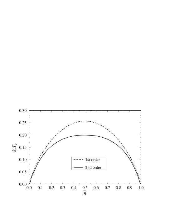
FIG. 4.: Curie temperature $T_{C}$ (in units of $t_{0}$) of the one-orbital double exchange model obtained using the first- and second-order expression for the $T$-matrix with respect to the fluctuations $\Delta{\cal H}$ as a function of averaged electronic density.

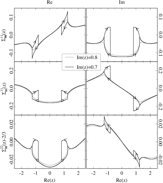
FIG. 5.: Behavior of matrix elements of the self energy in the paramagnetic state of degenerate double exchange. For ${\rm Im}(z)$$\geq$$0.75$ there is only one solution, while for ${\rm Im}(z)$$<$$0.75$ one can obtain two self-consistent CPA solutions in certain interval of ${\rm Re}(z)$ by starting the iterations with the self energy obtained for the previous value of ${\rm Re}(z)$ and moving either in the positive or negative direction of the real axis (shown as a hysteresis).

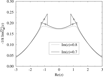
FIG. 6.: Imaginary part of the Green function (the local density of states) for the paramagnetic state of degenerate double exchange model. See Fig. 5 for description.

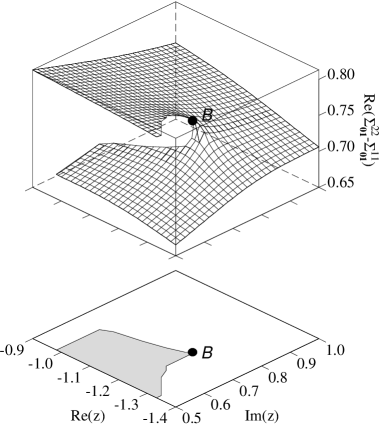
FIG. 7.: Topology of the non-local part of the self energy in the complex plane. The branch-point is denoted by $B$. The projection shows an approximate position of the double-valued area for the CPA solutions.

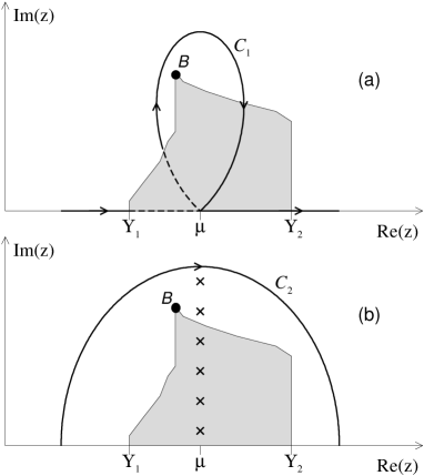
FIG. 8.: Energy integration for the degenerate double exchange model. (a): The integral along the real axis plus the discontinuity given by the contour integral $C_{1}$ around the branch-point $B$. (b): An equivalent expression in terms of the contour integral $C_{2}$ spreading in the single-valued area of the complex plane and residues calculated at Matsubara poles. The latter contributions are different for two different branches, that is equivalent to the discontinuity term in the scheme (a).

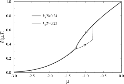
FIG. 9.: Averaged electronic density as a function of chemical potential for the paramagnetic state of degenerate double exchange model. For $T$$\leq$$0.23$, $\overline{n}(\mu)$ may take two different value for the same chemical potential $\mu$ which correspond to two different CPA solutions shown in Fig. 5.

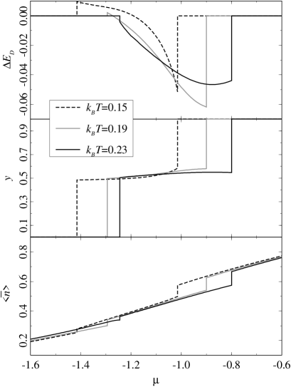
FIG. 10.: Pseudo-alloy picture for the two-phase paramagnetic state of the degenerate double exchange model: the change of the double exchange energy $\Delta E_{D}$$=$$E^{(2)}_{D}$$-$$E^{(1)}_{D}$, the equilibrium alloy concentration $y$, and the density of $e_{g}$ electrons averaged simultaneously over the spin orientations and the alloy concentrations $\langle\overline{n}\rangle$$=$$(1$$-$$y)\overline{n}^{(1)}$$+$$y\overline{n}^{(2)}$ as a function of chemical potential $\mu$ for three different temperatures (in units of $dd\sigma$-integral). The superscripts ⁽¹⁾ and ⁽²⁾ stand for the phases correspondingly with lower and higher electronic densities.

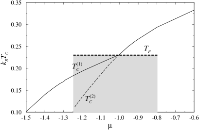
FIG. 11.: Main transition temperatures for the degenerate double exchange model (in units of $dd\sigma$-integral). $T_{P}$ is the transition temperature to the two-phase paramagnetic state. The shaded area shows the approximate range of the chemical potentials ($\mu$) when the paramagnetic state becomes intrinsicly inhomogeneous. $T_{C}^{(1)}$ and $T_{C}^{(2)}$ are the Curie temperatures for two different phases (characterized by lower and higher densities of the $e_{g}$ electrons, respectively).

REFERENCES

- [1] C. Zener, Phys. Rev. 82, 403 (1951).
- [2] P. W. Anderson and H. Hasegawa, Phys. Rev. 100, 675 (1955).
- [3] P.-G. de Gennes, Phys. Rev. 118, 141 (1960).
- [4] E. Müller-Hartmann and E. Dagotto, Phys. Rev. B 54, R6819 (1996).
- [5] K. Kubo and N. Ohata, J. Phys. Soc. Jpn. 33, 21 (1972).
- [6] R. Kilian and G. Khaliullin, Phys. Rev. B 60, 13458 (1999); S. Okamoto, S. Ishihara, and S. Maekawa, ibid. 61, 451 (2000); M. S. Laad, L. Craco, and E. Müller-Hartmann, ibid. 63, 214419 (2001).
- [7] A. Georges, G. Kotliar, W. Krauth, and M. J. Rozenberg, Rev. Mod. Phys. 68, 13 (1996).
- [8] N. Furukawa, in Physics of Manganites, ed. by T. A. Kaplan and S. D. Mahanti (Kluwer/Plenum, New York, 1999).
- [9] A. Chattopadhyay, A. J. Millis, and S. Das Sarma, Phys. Rev. B 61, 10738 (2000).
- [10] B. L. Gyorffy, A. J. Pindor, J. B. Staunton, G. M. Stocks, and H. Winter, J. Phys. F 15, 1337 (1985).
- [11] T. Oguchi, K. Terakura, and N. Hamada, J. Phys. F: Met. Phys. 13, 145 (1983).
- [12] Perhaps the absolute value of is not a serious problem as it can be easily adjusted by adding a phenomenological AFM SE interaction between the localized spins.[30, 46] The situation with the doping-dependence appears to be more serious. The experimental is not monotonous and has a maximum around (in La1-xSrxMnO3).[13] The maximum does exist in the one-orbital DE model (at ).[8] However, it is only an artifact of the one-orbital description, whereas in a more realistic DE model decreases as the function of .[46]
- [13] A. Urushibara, Y. Moritomo, T. Arima, A. Asamitsu, G. Kido, and Y. Tokura, Phys. Rev. B 51, 14103 (1995).
- [14] Y. Tomioka and Y. Tokura, Chapter 8 in Ref. [24].
- [15] M. Uehara, S. Mori, C. H. Chen, and S.-W. Cheong, Nature 399, 560 (1999).
- [16] M. Fäth, S. Freisem, A. A. Menovsky, Y. Tomioka, J. Aarts, and J. A. Mydosh, Science 285, 1540 (1999).
- [17] J. W. Lynn, R. W. Erwin, J. A. Borchers, Q. Huang, A. Santoro, J-L. Peng, and Z. Y. Li, Phys. Rev. Lett. 76, 4046 (1996).
- [18] A. J. Millis, P. B. Littlewood, and B. I. Shraiman, Phys. Rev. Lett. 74, 5144 (1995); A. J. Millis, Nature 392, 147 (1998).
- [19] S. Ishihara, M. Yamanaka, and N. Nagaosa, Phys. Rev. B 56, 686 (1997); Y. Tokura and N. Nagaosa, Science 288, 462 (2000).
- [20] A. Moreo, M. Mayr, A. Feiguin, S. Yunoki, and E. Dagotto, Phys. Rev. Lett. 84, 5568 (2000).
- [21] C. M. Varma, Phys. Rev. B 54, 7328 (1996).
- [22] I. V. Solovyev and K. Terakura, to be published in Electronic Structure and Magnetism of Complex Materials, ed. by D. J. Singh (Springer-Verlag, Berlin, 2002)
- [23] J. C. Slater and G. F. Koster, Phys. Rev. 94, 1498 (1954).
- [24] Colossal Magnetoresistive Oxides, ed. by Y. Tokura (Gordon and Breach Science Publishers, Tokyo, 2000).
- [25] M. O. Dzero, L. P. Gor’kov, and V. Z. Kresin, Solid State Commun. 112, 707 (1999); Eur. Phys. J. B 14, 459 (2000).
- [26] E. L. Nagaev, Physics–Uspekhi 38, 497 (1995); ibid. 39, 781 (1996).
- [27] E. Dagotto, S. Yunoki, A. L. Malvezzi, A. Moreo, J. Hu, S. Capponi, D. Poilblanc, and N. Furukawa, Phys. Rev. B 58, 6414 (1998); A. Moreo, S. Yunoki, and E. Dagotto, Science 283, 2034 (1999).
- [28] B. G. Nickel and W. H. Butler, Phys. Rev. Lett. 30, 374 (1973).
- [29] R. J. Elliott, J. A. Krumhansl, and P. L. Leath, Rev. Mod. Phys. 46, 465 (1974).
- [30] J. L. Alonso, L. A. Fernández, F. Guinea, V. Laliena, and V. Martín-Mayor, Phys. Rev. B 63, 054411 (2001).
- [31] Formally, the correlations can be included in a systematic way by adding corresponding terms to the trial Hamiltonian, which specifies the form of the distribution function (2).[10, 57, 58] However, it makes the calculations costly, and the main idea – less transparent. Therefore, at the first stage we neglect the correlations.
- [32] Note for example that the straightforward averaging of the Hamiltonian (1) with the distribution functions (2) will lead to an unphysical result: since is not symmetric function of , the self energy and the electron free energy will include odd contributions of .
- [33] Note that the PM-FM transition for the pure DE model is typically of the second order (perhaps except only the low density region). However, an additional AFM SE interaction between the spins can lead to the first-order transition and the phase coexistence: J. L. Alonso, L. A. Fernández, F. Guinea, V. Laliena, and V. Martín-Mayor, Phys. Rev. B 63, 064416 (2001).
- [34] F. Ducastelle, J. Phys. C: Solid State Phys. 8, 3297 (1975).
- [35] P. Bruno, J. Kudrnovský, V. Drchal, and I. Turek, Phys. Rev. Lett. 76, 4254 (1996).
- [36] N. Hamada and H. Miwa, Progr. Theor. Phys. 59, 1045 (1978).
- [37] M. H. Hettler, M. Mukherjee, M. Jarrell, and H. R. Krishnamurthy, Phys. Rev. B 61, 12739 (2000).
- [38] G. Kotliar, S. Y. Savrasov, G. Pálsson, and G. Biroli, Phys. Rev. Lett. 87, 186401 (2001).
- [39] I. V. Solovyev and K. Terakura, Phys. Rev. B 63, 174425 (2001).
- [40] A. I. Lichtenstein and M. I. Katsnelson, Phys. Rev. B 62, R9283 (2000).
- [41] Some results of the orientational averaging with the distribution function (4):[3] , , and for .
- [42] For example, the requirement is not fulfilled for all . Note however, that in order to formulate the CPA equations, the Green function was truncated in the real space after the nearest neighbors. Therefore, for all , which is equivalent to the knowledge of all elements of the Green function in the real space, appears to be an ill-defined quantity. Thus, the requirement is not generally applicable in the case of non-local CPA.
- [43] The factor ’6’ in the second term of Eq. (16) stands for the coordination number and the sign ’’ is related with the definition of the non-local part of the self energy – see Eq. (9).
- [44] The energy integration in Eq. (17) is rather straightforward. For example, the integral along the real axis can be replaced by a contour integral in the upper half plane plus contributions coming from residues calculated at Matsubara poles , 0, 1, 2, …[51]
- [45] In fact, different authors reported somewhat different estimates for based on the DMFT. The value reported in Ref. [48] for in units of the half bandwidth would roughly correspond to . On the other hand, the values and reported in Ref. [59] for and would yield and , respectively. In any case, all these values are higher than the ones obtained in the non-local CPA approach in the present work.
- [46] M. O. Dzero, Solid State Commun. 117, 589 (2001).
- [47] Note, that by combining the DE model with the phenomenological SE interaction between nearest neighbors in the form , the Curie temperature can be reduced, in the mean-field approximation, as . In three-dimensional manganites MnO3, the exchange constant can be estimated (from the low-temperature spin-wave dispersion) as - meV.[22]
- [48] Y. Motome and N. Furukawa, J. Phys. Soc. Jpn. 69, 3785 (2000); ibid. 70, 3186 (2001).
- [49] V. Heine and J. H. Samson, J. Phys. F: Metal Phys. 13, 2155 (1983).
- [50] In these calculations, we start CPA iterations at the point , with two self-consistent solutions corresponding to one of such points, say , which were obtained in advance, and move along the imaginary axis until the merging of two solutions.
- [51] K. Wildberger, P. Lang, R. Zeller, and P. H. Dederichs, Phys. Rev. B 52, 11502 (1995).
- [52] In practical terms, we start the iterations at with two different sets for the self energy, which guarantee two different CPA solutions, and then at each consecutive pole start with the self-consistent CPA solutions obtained for (and so on until merging of the two solutions).
- [53] Eq. (36) is obtained by using the Lloyd formula for the integrated density of states and is nothing but the generalization of Eq. (16) for the two-orbital case, which includes also the trace over the orbital indices. The latter is responsible for the factor ’2’ in the first term and gives rise to the two contributions in the second term of Eq. (36).
- [54] In this sense, our scenario is qualitatively different from the FM-PM phase separation encountered in the one-orbital DE model with an additional AFM SE interaction, which typically accompanies the discontinuous (first-order) phase transition to the FM state.[30, 33]
- [55] Y. Tomioka, private communication.
- [56] The choice of the FM phase was general from the viewpoint of the pure DE model, where the FM ground state at is the only possibility. However, the assignment was not sufficiently general from the viewpoint of possible modifications of the DE model, including the AFM SE interactions between the localized spins, for example.
- [57] S. V. Tyablikov, Methods of quantum theory of magnetism (Nauka, Moscow, 1975).
- [58] M. Uhl and J. Kübler, Phys. Rev. Lett. 77, 334 (1996).
- [59] A. J. Millis, Chapter 2 in Ref. [24].