Aging phenomena in nonlinear dissipative chains: Application to polymer.

Abstract

We study energy relaxation in a phenomenological model for polymer built from rheological considerations: a one dimensional nonlinear lattice with dissipative couplings. These couplings are well known in polymer’s community to be possibly responsible of $\beta$-relaxation (as in a Burger’s model). After thermalisation of this system, the extremities of the chain are put in contact with a zero-temperature reservoir, showing the existence of surprising quasi-stationary states with non zero energy when the dissipative coupling is high. This strange behavior, due to long-lived nonlinear localized modes, induces stretched exponential laws. Furthermore, we observe a strong dependence on the waiting time t_w after the quench of the two-time intermediate correlation function C(t_w+t, t_w). This function can be scaled onto a master curve, similar to the case of spin or Lennard-Jones glasses.
Keywords:
Localization of energy, Polymer, Breather modes, Stretched exponential, Lattices, Glasses.

1 Introduction

An important challenge in polymers physics nowadays is the understanding of non-equilibrium glassy state and associated slow relaxations ediger . At temperature below the liquid-to-glass transition temperature, the structural relaxation time depends indeed on the time spent in the glassy phase, the so-called waiting time $t_{w}$: this is the aging effect struck ; young ; bellon . Low-frequency mechanical spectroscopies show two different slow relaxations, namely $\alpha$ and $\beta$, corresponding to two different temperatures T${}_{\alpha}>$ T_β which depend on the mechanical excitation frequency; T_α is shown to be very close to the liquid-to-glass transition temperature ediger . Both relaxation modes are characterized by a maximum of dissipation but are surprisingly differently affected by physical aging: strongly for the first one but very weakly for the second. In spite of many studies, the microscopic origin of liquid-to-glass transition and of these relaxation modes are not yet well established conf . The $\alpha$ relaxation, associated to the liquid-to-glass transition, involves cooperative motions inducing an increase of the viscosity, whereas localized motions would be responsible of the $\beta$ relaxation with a clamping of degrees of freedom (for instance macromolecule rotation) near the temperature T_β.

Some phenomenological models (for instance Burger, Maxwell, Kelvin-Voight or Zener’s models) have been developed using linear viscoelastic theory ferry ; eirich and describe easily some aspects of relaxation in spite of their simplicity. These systems (see for example Burger’s model in Fig. 1a) correspond to a succession of springs and viscous elements (dashpots) set in parallel or in series, to modelize interactions between and inside polymers. As we will see in Section 2, in the case of Burger’s system, the dashpot with viscous parameter $\gamma_{1}$ (which modelized viscous interaction between molecules) is linked to $\alpha$ relaxation (and therefore to liquid-to-glass transition), whereas the second piston (which modelized a dissipative interaction inside the molecules) induces $\beta$ relaxation. Let us notice that these simple dynamical models don’t exhibit any physical aging. One way to describe and explain this phenomenon could be that of taking into account nonlinear interactions inside macromolecules.

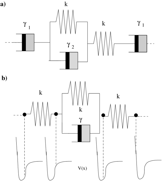
Figure 1: Sketch of the Burger’s linear model (panel a), and of our non-linear dissipative model for polymers (panel b).

Indeed, one of the most important feature of nonlinear systems is the localization of vibrational energy (named discrete breather) that modifies strongly the energy relaxation aubry ; reigada and induces non-equilibrium dynamics. Brea-thers are known to have very interesting dynamical properties and have been used in explaining a variety of physical and biophysical phenomena. For instance in nonlinear systems where breathers become mobiles, they could contribute directly to the energy transfer and modify its relaxation properties in a nonexponential dependance. This interesting phenomenon has been invoked in several physical settings as DNA molecules peyrard , hydrocarbon structures kopidakis , targeted energy transfer between donors and acceptors in biomolecules aubry2 . When the coupling is much smaller than the non linearity, the presence of essentially pinned long-lived breathers in nonlinear systems blocks the energy propagation aubry . The macroscopic manifestation of this phenomenon is a very slow relaxation of the total energy, reminiscent of the long lifetime of metastable states in glassy systems observed after a quench.

The case of relaxation phenomena in nonlinear lattices with bulk dissipation (as in glassy polymers) has received much less attention, though the experimental systems belong to this class marin . Indeed, the $\beta$ relaxation in glassy polymers, which is characterized by a maximum of dissipation, may be induced by the clamping of degrees of freedom. In spite of this dissipative effect, physical aging of this system is very slow. Understand this strange behavior is one of the aims of this paper. To accomplish this goal, we will examine the influence in energy relaxation of a dissipative coupling by performing numerical studies on a phenomenological model of polymers. The system, described in Section 3 and pictured in Fig. 1b, corresponds to particles coupled via elastic and dissipative interactions (as in Burger’s model for the molecular modelization); in addition, each particle is submitted to an on-site nonlinear potential to take into account interactions between different polymers including several contributions such as hydrogen bonds linking and repulsion of two chains (short-range steric restrictions). For a fixed viscous parameter $\gamma$, we examine the relaxation of energy when, after thermalization, the ends of the chain are placed in contact with a zero-temperature reservoir. Results show different kinds of energy relaxation regime which depend strongly of the dissipative terms: in particular, we show that the system can relax very slowly in spite of high dissipative couplings!

2 Viscoelastic systems and $\alpha$, $\beta$ relaxations

In many experimental studies, isochronal dynamical mechanical spectrometry has been performed at different frequencies ediger . With these measures, it is possible to map the loci of $\alpha$ and $\beta$ relaxations (defined by maximum of the imaginary parts of shear modulus G=G’+iG”) versus temperature and frequency. Typically, the $\alpha$-relaxation process exhibits a clearly non-Arrhenius behavior above the liquid-to-glass transition T_g, whereas an Arrhenius behavior is observed for temperature below T_g, when the system is out of thermodynamical equilibrium. The second process $\beta$ appears at higher frequencies than $\alpha$-process with also an Arrhenius behavior.

It is well-known in polymer’s community that some aspects of the rheology of glassy polymers can be described easily by using phenomenological models from viscoelastic linear theory ferry ; eirich ; turner . It can be assumed that the deformation of the polymer is divided into elastic and viscous components and can be described by a combination of Hooke and Newton’s laws. These systems correspond to springs and dashpots, either in series or in parallel. The Burger’s model (one element is described in Fig. 1a) seems to be a good candidate to illustrate the rheological behavior of polymers in glassy state. One element is made of two springs in series to modelize the chain of a macromolecule. In addition, one part of this chain is coupled in parallel with a dashpot to take into account the clamping of some degrees of freedom at low temperature, inducing the $\beta$-relaxation. The second dashpot in series with elastics components illustrates the viscous behavior of the system when it becomes glassy and induces the $\alpha$-relaxation.

In this model, the shear modulus G=G’+iG” is measured by applying a sinusoïdal force, with frequency $\omega$, at one end of a chain with 100 elements and by fixing the other extremity. G is the ratio between the applied force and the relative displacement of the chain extremity obtained in the stationary limit. The shear modulus is determined in a temperature window by using two Arrhenius laws for the viscosity $\gamma_{1}$ and $\gamma_{2}$:

$$\gamma_{1}=\gamma_{1}^{0}\ e^{E/k_{b}T}$$ (1)

and $\gamma_{2}=10^{-5}\gamma_{1}$. Furthermore, as in all viscoelastic linear studies (see for instance references  ferry ; eirich ; turner ) there is no inerty inside the system: each connection between springs and dashpots is considered as a particule with a mass equal to zero.

In Fig. 2, we report the evolution with temperature of the shear moduli G’, G” and loss tangent $\tan\phi$=G”/G’ for parameters given in the corresponding caption. These curves show two distinct regions of rheology, namely for increasing temperature, the $\beta$-process (weak decreasing of G’ and, maxima of G” and $\tan\phi$) and the $\alpha$-process (strong decreasing of G’ and maximum of G”). This behavior is qualitatively similar to those observed experimentally ferry . However, some differences appear. The loss tangent exhibits an increase with temperature for the $\alpha$-process, but we don’t observe a maximum unlike in experimental measurements. Furthermore, for temperature higher than the liquid-to-glass transition temperature, a non-Arrhenius behavior is observed experimentally for the $\alpha$-relaxation. This characteristic is not take into account in the evolution of $\gamma_{1}$.

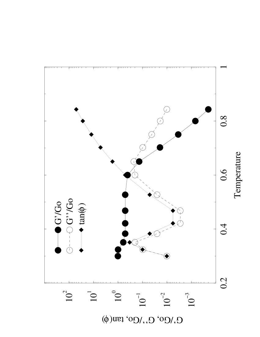
Figure 2: Values of the real (G’) and imaginary (G”) parts of shear modulus and of $\tan\phi$; they are plotted versus temperature for the Burger’s model of Fig. 1a. The shear moduli are divided by the modulus limit of low temperature G₀. Parameters used in the calculations are k=0.1, $\gamma_{1}^{0}$=10⁶, E/k_b=9.7 and $\omega$=10^-2.

In spite of these differences, the major overriding conclusion for this section is the possibility to observe rheological characteristics, like $\beta$-process, of the glassy state by considering a viscous coupling inside the molecule (linked to the rotation of terminal groups or other side chain motions ferry ). This modelization is however very concise and it is not possible to describe any aging phenomena because of the linearity of components.

In the next part, we will describe a phenomenological model including dissipative couplings and nonlinear interactions that may modelize more precisely one chain of a macromolecule. The main question we would like to address is the possibility to observe a long lived non-equilibrium state in nonlinear systems despite dissipative terms. In order to solve this problem, we simplify the system: the initial thermalized nonlinear system is put in a zero-temperature bath with a fixed viscous parameter independent of temperature.

3 The phenomenological dissipative nonlinear model

We consider a one dimensional chain of N=200 anharmonic oscillators, with a nonlinear on-site potential V(x), with free ends and nearest-neighbor elastic coupling potential (the coupling being k). The sketch of the chain is reported in Fig. 1b. In analogy with Burger’s model and in order to modelize the clamping degree of freedom, we consider for one half of nearest-neighbors a dissipative coupling ($\gamma$ is the dissipative parameter) in parallel with elastic coupling. For the on-site potential V(x), describing the interactions between two molecules (hydrogen long-range attraction and steric short-range repulsion), we have chosen the Morse potential

$$\mathrm{V(x)=\frac{1}{2}[1-e^{-x}]^{2}}$$ (2)

which has the appropriate shape to describe the strong repulsion when the chains are pushed toward each other (x$<$0) and the vanishing interaction when the chains are pulled very far apart (x$\gg$1). Each end oscillators of our chain can be also submitted to an additional damping force. The equations of motion of this chain are given in dimensionless form by:

$$\mathrm{\ddot{x}_{2i}} = \mathrm{-\frac{\partial V}{\partial x_{2i}}-k(2x_{2i}-x_{2i+1}-x_{2i-1})}$$ (3)

$$\mathrm{-\gamma(\dot{x}_{2i}-\dot{x}_{2i-1})-\gamma^{\prime}\dot{x}_{2i}\delta(2i-200)}$$

and

$$\mathrm{\ddot{x}_{2i+1}} = \mathrm{-\frac{\partial V}{\partial x_{2i+1}}-k(2x_{2i+1}-x_{2i}-x_{2i+2})}$$ (4)

$$\mathrm{-\gamma(\dot{x}_{2i+1}-\dot{x}_{2i+2})-\gamma^{\prime}\dot{x}_{2i+1}\delta(i)}$$

where x_n is the dimensionless displacement of the nth oscillator from equilibrium, $\dot{x}_{n}$ its velocity and $\delta$ the Kronecker delta function. The mass of the oscillators is set to unity by appropriately renormalizing time units. The equations of motion have been integrated using a fourth order Runge-Kutta method.

To study energy relaxation, we consider k=0.01 and we initially thermalize the system at temperature T=1 by using Nos$\mathrm{\acute{e}}$-Hoover thermostats nose . This temperature is much higher than the critical temperature (T_c=0.2) of the ”order-disorder” transition which characterizes the non dissipative model $\gamma$=0 (for more detail see references theo ; dau ). Then, in average, the kinetic energy per site is higher than the depth of Morse potential (which is equal to 0.5 in our arbitrary units) and we can consider our system as in an initial ”liquid” state: all the particules are in the plateau of the Morse potential. In other words, there are no interaction between chains of molecules. The thermalization procedure is performed with $\gamma$=$\gamma$’=0 by using a chain of three thermostats to provide a good exploration of the phase space nose .

After thermalization, the connection with the heat bath is turned off and the lattice is connected to a zero temperature reservoir via the damping term with $\gamma$’=0.1. However, we explore the interval [0,100] for the dissipative parameter $\gamma$. As our purpose is to search for long lived non-equilibrium state in spite of dissipative couplings, we prefer to simplify the problem and not to consider a temperature dependence of $\gamma$ like in the Burger’s model of section 2. The moment of connection with the zero temperature reservoir is chosen as the origin of time. At each step of the integration of equations (2) and (3), we evaluate the total lattice energy:

$$\mathrm{E=\sum_{i=1}^{200}\left[\frac{1}{2}{\dot{x}_{i}}^{2}+V(x_{i})\right]+\sum_{i=1}^{199}\frac{k}{2}(x_{i+1}-x_{i})^{2}}$$ (5)

and consider the symmetrized local energy per site:

$$\mathrm{E_{i}=\frac{1}{2}{\dot{x}_{i}}^{2}+V(x_{i})+\frac{k}{4}(x_{i-1}-x_{i})^{2}+\frac{k}{4}(x_{i}-x_{i+1})^{2}}\quad.$$ (6)

Total energy is expected to decrease with time and converge to a zero value of the ”frozen” state at equilibrium.

4 Relaxation of the thermalized system

In Fig. 3, we report the total lattice energy divided by the initial energy versus time for various viscous parameter $\gamma$. For $\gamma$=0, a clear non exponential decreasing energy is observed, consistent with Tsironis and Aubry’s results aubry . This long-tail relaxation behavior was shown by these authors to be connected to the presence of long-lived non linear localized modes that are relatively mobile. If we consider a small dissipative coupling ($\gamma$=10^-3) inside the lattice, we see that total energy decreases faster than previously. This small dissipative coupling induces a strong modification of energy relaxation to the ”frozen” state (normalized energy closed to 0) for a time smaller than 10⁴ (in arbitrary units). This emphasizes that the dissipative couplings change strongly the relaxation mechanisms and can induce a fast relaxation regime.

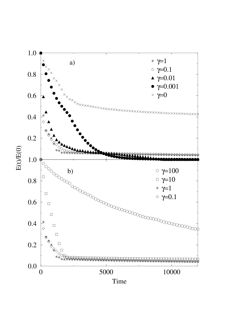
Figure 3: Normalized total energy decay as function of time for various viscous parameter $\gamma$. Initially each array is in thermal equilibrium at the temperature T=1.

For $\gamma$ higher than 0.1, a new surprising feature is observed: normalized energy seems to be blocked with a very slow decrease for long time whereas the dissipative parameter is higher! The system seems to evolve in a quasi-stationary state that is neither a ”frozen” state (the normalized energy is clearly different from 0) nor a ”liquid” state” (energy is too low). We can also notice that, at a given time, the energy of this quasi-stationary state increases with $\gamma$. This situation seems to be qualitatively similar to polymer systems where a very long-lived non-equilibrium glassy state is observed with very slow physical aging for temperature smaller than T_α (the viscous parameter which follows an Arrhenius law is higher for lower temperature).

In previous relaxation studies in non linear lattices where blocking energy was observed, it has been shown that such behavior may be induced by long-lived breathers aubry . In order to examine more precisely the present situation, we report in Fig. 4 the spatiotemporal energy landscape of the lattice by plotting the local energy E_i in each lattice site for $\gamma=10^{-3},10^{-1}$ and 10. Time advances along the y axis until t=10⁴ and a gray scale is used to represent the local energy with darker shading corresponding to more energetic regions. For $\gamma$=10^-3, we can see two kinds of energy relaxation: on the one hand, there is a dissipation of the energy inside the lattice, characterized by a ”fibrous structure” of the local energy landscape in Fig. 4c and, on the other hand, we observe a dissipation of mobile breather via surface damping characterized by ”dark oblique lines”. For $\gamma\geq$0.1, we notice the clear presence of pinned long-lived breathers, responsible of the energy relaxation blocking. This localisation of energy is observed after a short time where energy not only decreases via the surface damping but also via a dissipation inside the lattice (see for example the landscape for $\gamma=10^{-1}$ and t$<$2500). Furthermore, these states have a very long lived time and are still observed for t higher than 10⁵.

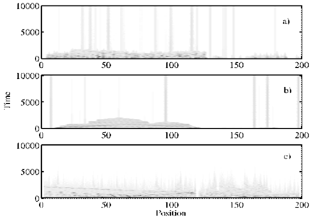
Figure 4: Evolution of the local energy E_i along the chain for various viscous parameter $\gamma$=10 (panel a), 0.1 (panel b) and 0.001 (panel c). The grey scale goes from E_i=0 (white) to the maximum E_i-value (black).

We have mentioned previously that, at early times, phonons and mobile breathers dissipation takes place before pinned breathers relaxation. Typically the hierarchy of relaxations processes may be classify in a sequence of characteristic times t${}_{1}^{*}<$t${}_{2}^{*}<$… tsang , where the energy relaxation corresponds approximately to exponential or a stretched exponential decay bibaki . Let us introduce the phonon relaxation time t^∗ defined by E(t^∗)/E(0)=0.5 which is characteristic of the phonon and mobile breather dissipation inside the lattice. We have reported in Fig. 5 the evolution of this relaxation time versus the viscous parameter $\gamma$. We clearly see, in this first step, that energy decreases faster for $\gamma$ between 0.1 and 1. In the case of a linear lattice, the maximum of dissipation is predicted to correspond to a value of $\gamma$ which verifies $\gamma\omega\sim K+k$ where K corresponds to the coupling constant of the linearized Morse potential (K=1 in our case) and $\omega$ is the frequency of the phonon band that starts at the frequency $\mathrm{\sqrt{K}}$=1 and extends to $\mathrm{\sqrt{K+4k}}$$\sim$1.02. Therefore, in the case of linearized oscillator, we expect a maximum of dissipation for $\gamma$ close to 1 in agreement with what is reported in Fig. 5. It is thus very surprising to observe quasi-stationary states in a second regime whereas dissipative effects are important. We have to notice that this paradoxal effect is very similar to the situation observed in the case of $\beta$ relaxation of polymers in glassy state: a very slow physical aging in spite of the maximum of dissipation conf .

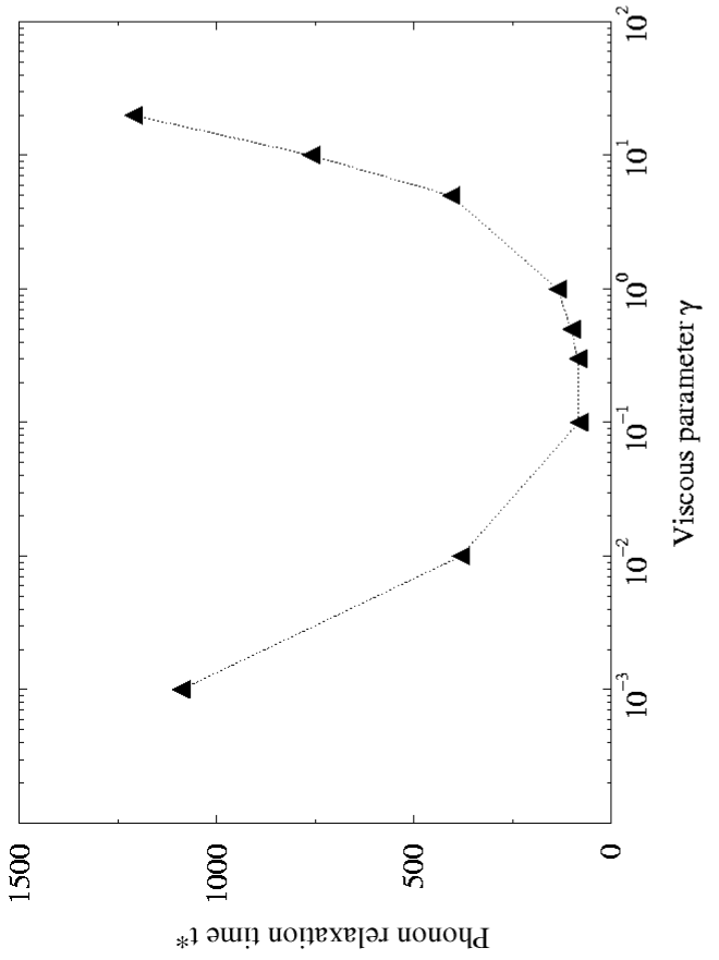
Figure 5: Phonon relaxation time t^∗, defined by E(t^∗)/E(0)=0.5, for various values of the viscous parameter $\gamma$.

In Fig. 6, we report the local energy in the lattice for various parameter $\gamma$ and at a given time t=2.$10^{4}$ much higher than the characteristic time of phonons and mobile breathers dissipation. For $\gamma$$<$0.1, the local energy per site is close to 0 as seen previously in Fig. 3: the system with small dissipative coupling reached thus rapidly an equilibrium frozen state. For $\gamma$$\geq$0.1, we clearly see the localization of energy, as long-lived breathers, in two nearest-neighbors oscillators dispatched in some areas of the lattice. We have verified that the two considered nearest-neighbors are coupled via piston: when $\gamma$ is high enough this coupling is clamped. In fact, the phase displacement of velocities of the both particles is very small, inducing a very slow dissipation and then referred a very long non-equilibrium state. The energy of these long-lived breathers is close to 0.5 at time t=2.$10^{4}$, and the associated sites are not linked with the on-site Morse potential. This quasi-stationary state is clearly not a frozen state, since some parts of a molecular chain are ”hot” but do not interact with other ones.

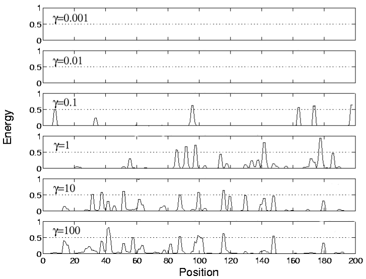
Figure 6: Instantaneous local energy E_i along the chain at time t=2.$10^{4}$ for various dissipative parameter $\gamma$. The dashed lines show the limit of Morse potential for large displacement x_i.

For t$\gg$t^∗ and $\gamma$$\geq$0.1, the energy relaxation of the quasi-stationary state can be very well fitted by a Kohlrausch-Williams-Watts function or stretched exponential function:

$$\mathrm{E(t)=E_{b}(0)e^{-(at)^{b}}}$$ (7)

where the coefficients a, b and E_b(0) are $\gamma$ dependent. E_b(0) can be qualified as the total energy of pinned breathers at time t=0. The Kohlrausch kohlrausch exponent b is a parameter measuring the deviation from a single exponential form (0$\leq$b$\leq$1). In Fig. 7, we have reported the evolution of [-lnE(t)/E_b(0)] versus t with logarithmic scales for various parameter $\gamma$$\geq$0.1. We can see a very clear linear dependance for high t (after phonon and mobile breather dissipation), which attests that this long-lived breather energy relaxes as a stretched exponential.

Figure 7: Log[-ln(E(t)/E_b(t))] versus log t for various dissipative parameter $\gamma$. The dashed lines are the stretched exponential fits.

We see also in these figures that the slope of the straight lines depends on the viscous parameter $\gamma$. In order to examine more precisely this dependence, we report in Fig. 8 the Kohlrausch exponent b versus the viscous parameter $\gamma$. We clearly see a maximum of the exponent b for values of $\gamma$ close to 0.5. The b-value is equal to 0.82 and then the energy relaxation differs from a pure exponential decay. Furthermore, this figure shows that the pinned breathers relaxation is slower for higher parameter $\gamma$. It is therefore qualitatively similar to the glassy state where a slower aging phenomena is observed for slower temperature (and then higher viscosity as we can see in the Burger’s model of section 2) struck .

Figure 8: Kohlrausch exponent b for various viscous parameter $\gamma$.

5 Out of equilibrium dynamic correlations

Studies of nonequilibrium systems like spin, structural or Lennard-Jones glasses young ; kob have shown that the nonequilibrium dynamics of the previously described states could be much efficiently characterized by two-time correlation functions of the form:

$$\mathrm{C(t_{w}+t,t_{w})} = \mathrm{\langle A(t_{w}+t)A(t_{w})\rangle}$$ (8)

$$\mathrm{-\langle A(t_{w}+t)\rangle\langle A(t_{w})\rangle}$$

where A is a microscopic observable, and t_w is the ”waiting time” i.e., the time elapsed after the quench. Brackets denote an average over different initial configurations at temperature T. At equilibrium, this two-time quantity satisfies time translation invariance and then depends only on the time t. On the other hand, in out of equilibrium situations, such equilibrium property is not verified: this function depends on the waiting time t_w (”aging effect”). The correlations functions for large times are expected to scale in the form:

$$\mathrm{C(t_{w}+t,t_{w})} = \mathrm{C_{ST}(t)+C_{AG}\left(\frac{\xi(t_{w}+t)}{\xi(t_{w})}\right).}$$ (9)

The first term describes short time dynamics that does not depend on t_w and has the equilibrium form. The second term, or aging part, depends only on the ratio $\xi$(t_w+t)/ $\xi$(t_w) where $\xi$(t) is a monotonous increasing function of t. In a lot of cases $\xi$(t)$\propto$t or $\propto$t^ν so that the aging part is simply a function of t/t_w and exhibits a master curve (see for instance, experiments on thermoremanent magnetization vincent , gels cipelletti or particle suspensions kroon ; knaebel ).

In this study we have considered the microscopic observable A(t)=$\mathrm{(\sum^{200}_{i=1}x_{i}(t))/200}$ that is the mean deformation per site of the chain at time t. Numerical calculations have been done in the case of a quench of the system with a viscous parameter $\gamma$=10 from temperature T=1 to T=0. Two-time correlation functions are obtained for various waiting time by considering 11 different initial configurations. Furthermore, in order to make a quantitative comparison, we prefer to calculate correlation normalized by C(t_w,t_w).

In Fig. 9, we have reported the evolution of normalized two-time correlations function C(t_w+t,t_w) versus time t for different waiting time (we consider t_w$\gg$t^∗ in order to study only long lived non equilibrium states after phonons and mobile breathers dissipation). The behavior of C clearly emphasizes the lost of time-translation invariance and the dependence on the waiting time t_w. This figure also shows that the dynamics can be decomposed into two time scales:

(i) at short time separation (t$<$20) correlation function doesn’t depend of t_w and is equal to the value expected at equilibrium (C=1 at T=0).

(ii) the decay from this value toward zero arises in a second time scale that clearly depends on t_w: the system does’nt reach equilibrium within the time window explored in the simulation. Furthermore we can notice that the larger the waiting time, the longer it takes the system to forget the configuration at time t_w. This behavior is typical of aging effect young .

Figure 9: Normalized non-equilibrium correlation function C(t_w+t,t_w) for fixed value t_w versus time t. The viscous parameter is $\gamma$=10 and from bottom to top the waiting times are t_w=5844, 9300, 14700, 23137, 36321, 56920, 71225.

Guided by equation (9) we test the scaling assumption for long times in Fig. 10, where normalized correlation functions are reported versus normalized time t/t_w. The different curves can be superimposed, indicating the validity of the scaling ansatz and the existence of a master curve. This striking feature is observed in many non-equilibrium systems vincent ; cipelletti ; kroon ; knaebel and is very similar with comparable studies on spin glasses young or Lennard-Jones glasses kob . The physical origin of this universal t/t_w scaling is, at this day, an open question. Kob and Barrat suggest in reference kob that it could be induced by a similarity of the geometry of phase space of these systems in spite of differences in microscopic dynamics.

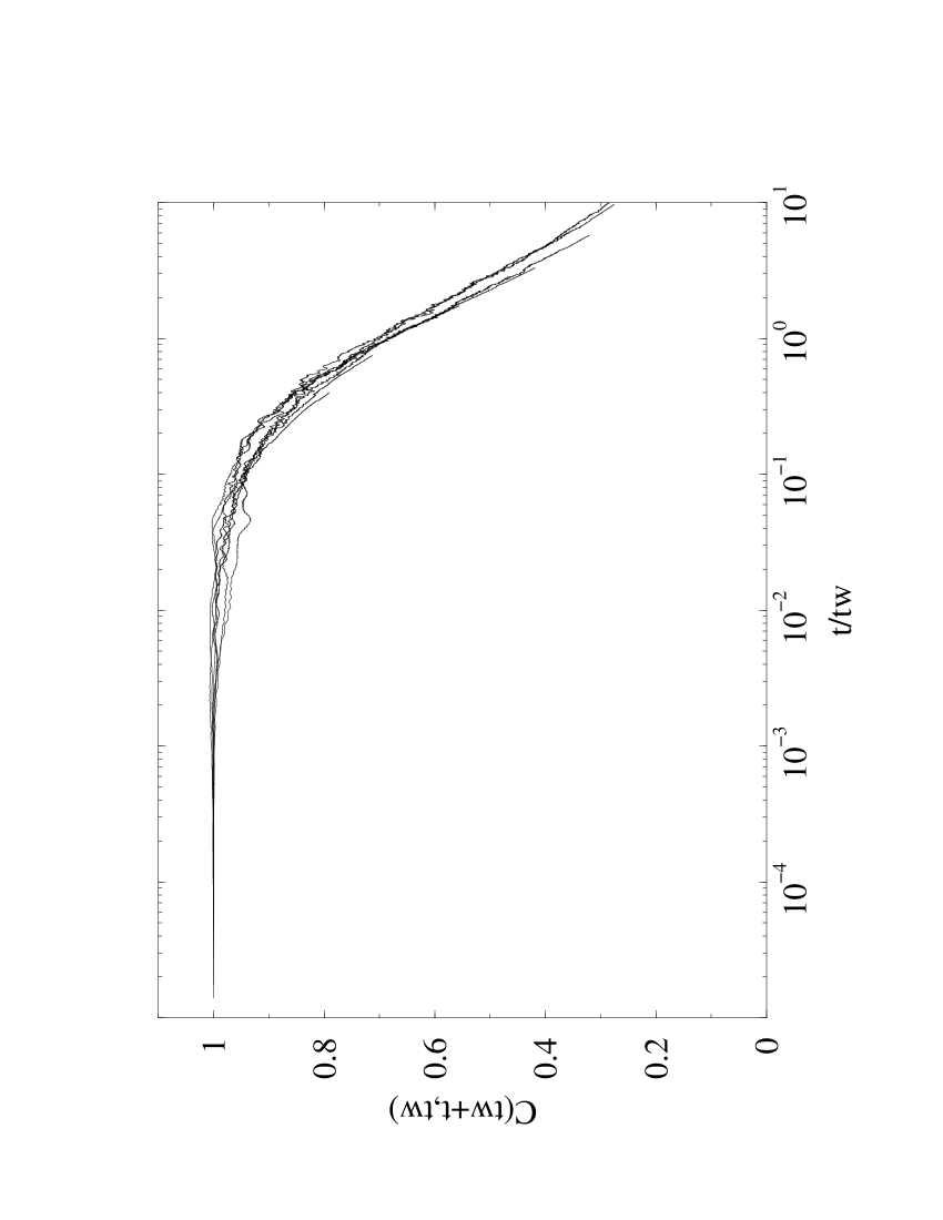
Figure 10: The data of Fig 9 versus t/t_w: master curve

Finally, we would like to point out that Fig. 9 shows also the violation of the dissipation-fluctuation theorem (FDT). It seems to be a characteristic of non-equilibrium system as observed numerically in domain growth process abarrat , Lennard-Jones glasses jlbarrat or slow granular rheology berthier and experimentally for dielectric measurements in colloidal glasses bellon1 , supercooled fluid grigera and polymer glasses herisson ; buisson . Let us consider the response R(t_w+t,t_w) to a field h conjugated to observable A. At equilibrium, response to this external field is given by FDT i.e., at equilibrium, the following equation is verified:

$$\mathrm{R(t_{w}+t,t_{w})} \equiv \mathrm{\left.\frac{\delta\langle A(t_{w}+t)\rangle}{\delta h(t_{w})}\right|_{h=0}}$$ (10)

$$= \mathrm{-\frac{1}{T}\frac{\partial C(t_{w}+t,t_{w})}{\partial t}}$$

and then:

$$\mathrm{\frac{\partial C(t_{w}+t,t_{w})}{\partial t}} = \mathrm{-T\ R(t_{w}+t,t_{w})}$$ (11)

where T is the bath temperature.

If we consider a quench at a zero-temperature bath (as in our case), then for satisfying FDT, normalized correlation function has to be constant:

$$\mathrm{C(t_{w}+t,t_{w})=C(t_{w},t_{w})=1\ \ ,\ \ \forall t\geq 0.}$$ (12)

Evolutions of correlation functions reported in Fig. 9 show clearly that C(t_w+t,t_w) is not a constant with time t: fluctuation-dissipation theorem is violated in this non-equilibrium system as seen in other glasses abarrat ; jlbarrat ; berthier ; bellon1 ; grigera ; herisson ; buisson . Moreover, the larger the waiting time, the longer it takes the system to violate the FDT.

6 Conclusion

Using simple rheological considerations and results from Burger’s model, we built a phenomenological model of a polymer-chain. This system is a one dimensional nonlinear lattice characterized by dissipative couplings. The energy relaxation studies of this thermalized system show that for sufficiently large viscous parameter $\gamma$, it is possible to observe nonequilibrium quasi-stationary states in spite of the short characteristic time of phonon dissipation! This surprising behavior is due to a chain auto-organisation which minimizes energy dissipation, inducing the clamping of some degrees of freedom and forming long-lived pinned breathers.

Moreover, this very slow energy relaxation can be fitted by stretched exponential laws, ubiquitous in glassy polymer aging properties. Another similarity with these physical systems is that this aging phenomenon is slower when the viscous parameter $\gamma$ is higher. Furthermore, the two-time correlation function C(t_w+t,t_w) shows a strong dependence on the waiting time and can be scaled onto a master curve by considering the evolution versus normalized time t/t_w.

By these aspects (clamping of degree of freedom, long-lived nonequilibrium state, stretched exponential decays, violation of time-translation invariance and master curve), the glassy nature of this simple dissipative non linear lattice is very similar to those observed in glassy polymers. Beside its interest for nonlinear physics, this model is presumably an alternative to study complex systems like glassy state polymers: we have now to push our investigations further by examining other properties like dependences on cycling temperature, evolution with waiting time of the shear moduli. Work along this line is in progress.

References

- (1) M. D. Ediger, C. A. Angell, S. R. Nagel, J. Phys. Chem. 388, 13200 (1996)
- (2) L. C. E. Struik, Physical Aging in Amorphous Polymers and Other Materials (Elsevier, Houston, 1978)
- (3) A. P. Young (Editor), Spin Glasses and Random Fields, Series on Direction in Condensed Matter Physics, 12, World Scientific, Singapore (1998)
- (4) L. Bellon, S. Ciliberto, and C. Laroche, Europhys. Lett. 51, 551 (2000)
- (5) See for examples International Conferences on Relaxation in Complex Systems: Heraklion, 1990, Proceedings published in J. Non-Cryst. Solids 131-133 (1991) 1-1266; Alicante, 1993, Proceedings published in J. Non-Cryst. Solids 170 (1994) 1-1440
- (6) J. D. Ferry, Viscoelastic Properties of Polymers (J.Wiley & Sons, New-York, 1980)
- (7) F. R. Eirich, Rheology (Academic Press Inc., New-York, 1956)
- (8) Turner Alfrey Jr, Mechanical behavior of high polymers (Interscience publishers, Inc., New York, 1948)
- (9) G. P. Tsironis, S. Aubry, Phys. Rev. Lett. 77, 5225 (1996)
- (10) R. Reigada, A. Sarmiento, K. Lindenberg, Phys. Rev. E 64, 066608 (2001)
- (11) M. Peyrard and J. Farago, Physica A 288, 199 (2000)
- (12) G. Kopidakis and S. Aubry, Physica B 296, 237 (2001)
- (13) S. Aubry, K. Kopidakis, e-print cond-mat/0102162
- (14) J. L. Marin, F. Falo, P. J. Martinez and L. M. Floria, Phys. Rev. E 63, 066603 (2001)
- (15) T. Dauxois, M. Peyrard and A. R. Bishop, Phys. Rev. E 47, 684 (1993)
- (16) G. J. Martyna, M. L. Klein, M. Tuckerman, J. Chem. Phys. 97, 2635 (1992)
- (17) N. Theodorakopoulos, T. Dauxois, M. Peyrard, Phys. Rev. Lett., 85, 6 (2000)
- (18) T. Dauxois, N. Theodorakopoulos, M. Peyrard, J. Stat. Physics, 107, 869 (2002)
- (19) K. Y. Tsang, K. L. Ngai, Phys. Rev. E, 54, R3067 (1996)
- (20) A. Bibaki, N. K. Voulgarakis, S. Aubry, G. P. Tsironis, Phys. Rev. E, 59, 1234 (1999)
- (21) R. Kohlrausch, Pogg. Ann. Physik. 12, 393 (1847)
- (22) W. Kob and J. L. Barrat, Phys. Rev. Lett. 78, 4581 (1997)
- (23) E.Vincent, J. Hammann, M. Ocio, J. P. Bouchaud and L. F. Cugliandolo, Slow dynamics and aging, edited by M. Rubi (Springer-Verlag, Berlin, 1997)
- (24) L. Cipelletti, S. Manley, R. C. Ball, D. A. Weitz, Phys. Rev. Lett. 84, 2275 (2000)
- (25) M. Kroon, G. H. Wegdam and R. Sprik, Phys. Rev. E 54, 6541 (1996)
- (26) A. Knaebel et al., Europhys. Lett. 52, 73 (2000)
- (27) A. Barrat, Phys. Rev. E, 57, 3629 (1998)
- (28) J. L. Barrat and W. Kob, Europhys. Lett. 46, 637 (1999)
- (29) L. Berthier, L. F. Cugliandolo and J. L. Iguain, Phys. Rev. E, 63, 051302 (2001)
- (30) L. Bellon, S. Ciliberto and C. Laroche, Europhys. Lett. 54, 511 (2001)
- (31) T. S. Grigera and N. E. Israeloff, Phys. Rev. Lett. 83, 5038 (1999)
- (32) D. Herisson and M. Ocio, Phys. Rev. Lett. 88, 257202 (2002)
- (33) L. Buisson, S. Ciliberto and A. Garcimartin, in preparation.