Designing agent-based market models

Abstract

In light of the growing interest in agent-based market models, we bring together several earlier works in which we considered the topic of self-consistent market modelling. Building upon the binary game structure of Challet and Zhang, we discuss generalizations of the strategy reward scheme such that the agents seek to maximize their wealth in a more direct way. We then examine a disturbing feature whereby such reward schemes, while appearing microscopically acceptable, lead to unrealistic market dynamics (e.g. instabilities). Finally, we discuss various mechanisms which are responsible for re-stabilizing the market in reality. This discussion leads to a ‘toolbox’ of processes from which, we believe, successful market models can be constructed in the future.

Oxford Center for Computational Finance working paper: OCCF/010702

1 Introduction

Agent-based models have attracted significant interest across a broad range of disciplines [1]. An increasingly popular application of these models has been the study of financial markets [1, 2]. The motivations for this focus on financial markets are two-fold: the promise that data-rich financial markets are good candidates for the empirical study of complex systems, and the inadequacy of standard economic models based on the notions of equilibria and rational expectations. Currently many different agent-based models exist in the Econophysics literature, each with its own set of implicit assumptions and interesting properties [1, 2, 3]. In general these models manage to exhibit some of the statistical properties that are reminiscent of those observed in real-world financial markets; for example, fat-tailed distributions of returns and long-timescale volatility correlations.  Despite their differences, these models draw on several of the same key ideas: feedback, frustration, adaptability and evolution. The underlying goal of all this research effort is to generate a microscopic agent-based model which (i) reproduces all the stylized facts of a financial market, and (ii) makes sense on the microscopic level in terms of financial market microstructure. While each of these goals is separately achievable, the combination of (i) and (ii) within a single model represents a fascinating challenge, and underpins our motivation for writing the present paper.

Challet and Zhang’s Minority Game [3] offers possibly the simplest paradigm for a system containing the key features of feedback, frustration and adaptability. The MG has remarkably rich dynamics, given the simplicity of its underlying binary structure, and has potential applications in a wide range of fields. Consequently Challet and Zhang’s MG model, together with the original bar model of Arthur [1], represent a major milestone in the study of complex systems. Given the MG’s richness and yet underlying simplicity, the MG has also received much attention as a financial market model [2]. The MG comprises an odd number of agents N choosing repeatedly between the options of buying (1) and selling (0) a quantity of a risky asset. The agents continually strive to make the minority decision i.e. buy assets when everyone else is selling and sell when everyone else is buying. This strategy seems to make sense on first inspection. For example, a majority of agents selling will force the price of the asset down and thus ensure a low buy price (which is favorable) for the minority of the agents who decided to buy; hence the minority group has ‘won’. However, now consider the scenario where this pattern repeats over and over. The minority of agents, who have been buying more and more assets as the price falls, now find themselves holding a huge inventory of assets which are worth very little. When these agents try to cash in their assets, they will find themselves very much poorer. Surely then the minority group has actually lost?

This paradox has sparked much discussion as to the suitability of the MG as the basis of a microscopic model of financial markets. Consequently a diverse range of modified (yet MG-related) models have emerged, all seeking to address this point in different ways [2]. Some models include a combination of different types of agents - in particular, agents who are rewarded for trading in the minority, and agents who are rewarded oppositely for trading in the majority (see Ref. [4] for an early example). In such models, the overall class of the game (minority or majority) is ambiguous, and is likely to change as differing numbers of each group flood in and out of the market. Other models try to combine the two different reward structures, thus requiring only one class of agents who strive to be neither exclusively in the minority group nor exclusively in the majority group [5, 6, 7]. We refer the reader to the Econophysics website [2] for further examples (see also Refs. [8, 9, 10, 11]).

The purpose of this paper is to consolidate the search for a suitable microscopic reward scheme for use in agent-based financial markets. The paper comprises a synthesis of several earlier reports, each aimed at addressing the topic of self-consistent agent-based market modelling within a binary game structure. These earlier reports are re-organized in light of several recent papers on specific reward structures, and supplemented by additional simulation results, observations and thoughts [7]. We start by discussing various strategy reward schemes in which the agents seek to maximize their wealth in a direct way. We then illustrate a disturbing feature whereby such reward structures, while appearing microscopically acceptable, can lead to unrealistic market dynamics (e.g. instabilities). Finally, we discuss various mechanisms which are responsible for re-stabilizing the market in reality. This discussion leads to a ‘toolbox’ of processes from which, we believe, successful market models can be constructed in the future.

2 Binary game structure

Consider the situation of a population of $N$ agents with some limited global resource. A specific example could be Arthur’s famous bar problem [1] where there are $N$ regular bar-goers but only $L<N$ seats. The reward scheme in Arthur’s bar problem is simple: bar-goers are successful if they attend and they manage to obtain a seat. This reward scheme implicitly assumes that the bar-goers value sitting down above other criteria. While this makes sense for many situations, it is not universal. For example, it is our experience that customers of college-based bars do not view seating as a necessary requirement for a successful evening! The motto ‘the more the merrier’ often seems more appropriate. The MG represents a very special case of the bar problem, in which the seating capacity $L=(N-1)/2$ and all the attendees wish to sit down. In more general and realistic situations, the correct reward scheme is likely to be less simple than either Arthur’s bar model or Challet and Zhang’s MG. Until a specific reward scheme is defined, the bar model remains ill-specified. Putting this another way, the precise reward scheme chosen is a fundamental property of the resulting system and directly determines the resulting dynamical evolution. Hence it is crucial to understand the effect that different microscopic reward schemes have on the macroscopic market dynamics.

As first discussed in Ref. [1], the bar problem is somewhat analogous to a financial market where the bar-goers are replaced by traders. In the same way that a general bar problem requires a non-trivial reward scheme, any ‘correct’ agent-based market model will need a non-trivial reward scheme in order to avoid inconsistencies with financial market microstructure. This provides us with the motivation to look beyond the bar model and MG, in order to design an agent-based model with financial relevance. Having said this, the binary structure of the MG provides an appealing framework for formulating a market model without introducing too many obvious pathologies. Given these considerations, our discussion from here on will not assume any specific reward scheme, but will employ a binary game structure based on Ref. [3].

We start by reviewing the binary game structure. There are three basic parameters; the number of agents $N$, the ‘memory’ of the agents $m$, the number of strategies held by each agent $s$. The agents all observe a common binary source of information, but only remember the previous $m$ bits. Hence the global information available to each agent at time $t$ is given by $\mu\left[t\right]$ where in decimal notation $\mu\left[t\right]\in\left\{0\ldots P-1\right\}$ with $P=2^{m}$. Each strategy $\underline{a}_{R}$ contains as its elements $a_{R}^{\mu}$, and represents a response $\left\{-1,1\right\}$ to each of the possible $P$ values of the global information $\mu$. There are hence $2^{P}$ possible strategies. The agents are randomly allocated a subset of $s$ of these strategies at the outset of the game, and are not allowed to replace these. The agents also keep a score $S_{R}$ reflecting their strategies’ previous successes, whether the strategy is played or not. The net action of the agents $A\left[t\right]$ is defined as:

$$A\left[t\right]=\sum_{R=1}^{2^{P}}n_{R}\left[t\right]a_{R}^{\mu\left[t\right]}$$

where $n_{R}$ is the number of agents playing strategy $R$. The agents always play their highest performing strategy, i.e. the strategy with the highest $S_{R}$. The strategy score is updated with payoff $g_{R}$ such that $S_{R}\left[t+1\right]=S_{R}\left[t\right]+g_{R}\left[t+1\right]$.

The central question is the following: what should we take as ‘success’ in the context of a market and hence what are the payoffs? In short, what is the microscopic reward scheme? This is equivalent to asking what the game actually is, since a game requires a definition of the players’ goals and hence their rewards. In order to address this question, we start by considering a binary version of Arthur’s bar problem with general $L$, i.e. an MG-like model which is generalized to $L\neq(N-1)/2$ [12, 13]. The two responses would be ‘attend’ or ‘don’t attend’, and there are two possible scenarios: (i) the attendance is less than the seating capacity. In this case, the attendees are successful while those who didn’t attend are unsuccessful. (ii) The attendance exceeds the seating capacity. In this case, the attendees are unsuccessful while those who didn’t attend are successful. Setting $L=(N-1)/2$ yields the MG, and the two scenarios collapse into one: the successful agents are those who predict the minority group, i.e. attend when the minority attend, or don’t attend when the majority attend. [For a study of the binary game with $L\neq(N-1)/2$, see Ref. [12, 13].] In the specific case of the MG, success is classified as having correctly predicted the minority outcome. The payoff function for the MG is thus of the form:

$$g_{R}\left[t+1\right]=\chi\left[-a_{R}^{\mu\left[t\right]}A\left[t\right]\right]$$ (1)

where $\chi\left[x\right]$ is an odd, increasing function of $x$ usually chosen to be either $\chi\left[x\right]=x$ or $\chi\left[x\right]=\operatorname*{sgn}\left[x\right]$. The feedback in the MG arises through the global information $\mu\left[t\right]$ where the most recent bit of the binary information is defined by the sign of the net action of the agents $A\left[t\right]$:

$$\mu\left[t+1\right]=2\mu\left[t\right]-P\operatorname{H}\left[\mu\left[t\right]-\frac{P}{2}\right]+\operatorname{H}\left[A\left[t\right]\right]$$ (2)

where $\operatorname*{H}\left[x\right]$ is the Heaviside function [14]. In the more general form of the game where the resource level $L\neq(N-1)/2$, the argument in the Heaviside function $\operatorname{H}\left[\dots\right]$ would depend on the value of $L$ [13]. More generally it could become a complicated function of all the game parameters, or include feedback from the macroscopic dynamics in the past, or even the effects of exogenous news arrival.

It is now accepted that a generalization of the MG in which agents can sit out of the game (i.e. $a^{\mu\left[t\right]}=0$) when they are not confident of the success of any of their $s$ strategies, provides a better model of financial trading since it allows the number of agents active in the market to vary. This more general model is the Grand Canonical Minority Game (GCMG) which was first studied in Ref. [11]. The GCMG typically has two more parameters than the MG: namely $T$ which is a time horizon over which strategy scores are forgotten (i.e. $S_{R}\left[t+1\right]=\left(1-1/T\right)S_{R}\left[t\right]+g_{R}\left[t+1\right]$) and $r$ which is a threshold value of $S_{R}$ below which the agents will opt not to participate in the game ($a^{\mu\left[t\right]}=0$). The GCMG seems to reproduce the stylized statistical features of a financial time-series over a wide parameter range (see the discussion in Ref. [15]).

3 The price formation process

It is commonly believed that in a financial market, excess demand (i.e. the difference between the number of assets offered and the number sought by the agents) exerts a force on the price of the asset. Furthermore it is believed that a positive excess demand will force the price up and a negative demand will force the price down. A reasonable suggestion for the price formation process could then be [16]:

$$\ln\left[p\left[t\right]\right]-\ln\left[p\left[t-1\right]\right]=\frac{D\left[t^{-}\right]}{\lambda}$$ (3)

or

$$p\left[t\right]-p\left[t-1\right]=\frac{D\left[t^{-}\right]}{\lambda}$$ (4)

where $D\left[t^{-}\right]$ represents the excess demand in the market prior to time $t$, when the new price $p\left[t\right]$ is set and the buy/sell orders are executed. The scale parameter $\lambda$ represents the ‘market depth’ (or liquidity) i.e. how sensitive a market is to an order imbalance. In general we would expect $\lambda$ to be some increasing function of the number of traders $N$ trading in that asset. Also, the functional forms may not be linear as in Equations 3 and 4. However, studies carried out on several markets have found the forms of Equations 3 and 4 to be reasonable [17].

In Ref. [4], we suggested that in markets involving a market-maker who takes up the imbalance of orders between buyers and sellers, the market-maker will wish to manipulate the price of the asset in order to minimize her inventory of stock $\phi_{M}\left[t\right]$. Whilst the market-maker’s job is to execute as many of the orders as is possible, she does not wish to accumulate a high position in either direction. To this end, the market-maker lowers the price to attract buyers when she holds a long position $\phi_{M}>0$ and raises it to attract profit-taking sellers when she has a short position $\phi_{M}<0$. This modifies the price formation of Equation 3 to:

$$\ln\left[P\left[t\right]\right]-\ln\left[P\left[t-1\right]\right]=\frac{D\left[t^{-}\right]}{\lambda}-\frac{\phi_{M}\left[t^{-}\right]}{\lambda_{M}}$$ (5)

where $\lambda_{M}$ is the market-maker’s sensitivity to her inventory.

4 From MG to market model

Our puzzle is to form a sensible model of a collection of traders buying and selling a financial asset. It is clear from Sections 2 and 3 that we have two pieces of the puzzle. The MG gave us a simple paradigm for a group of agents interacting in response to global information and adapting their behavior based on past experience. The output of this model was a ‘net action’ $A\left[t\right]$. In addition, we now have some simple systems for price-formation based on an excess demand $D\left[t\right]$. But what relationship should we assume between $D\left[t\right]$ and $A\left[t\right]$? To answer this question, we should clarify what we want the individual actions $a_{R}^{\mu\left[t\right]}$ of the strategies to resemble. In short, the question is ‘what does a strategy map from and to?’

In most studies of the MG as a market model, researchers have taken the actions $a_{R}^{\mu\left[t\right]}\in\left\{-1,1\right\}$ to be the actions of selling and buying a quanta of the asset respectively. Thus the net action of all agents $A\left[t\right]$ naturally becomes the excess demand, i.e. we have:

$$D\left[t^{-}\right]=A\left[t-1\right]$$ (6)

Given this and the fact that the price change is an increasing function of excess demand (for Equations 3 and 4), the global information becomes the directions (up or down) of the previous price changes. So the answer here is that a strategy maps from the history of past asset price movements to a buy/sell signal. A strategy mapping from the history of past asset price movements seems a natural and sensible choice, since financial chartists do look at precisely this information to decide upon a course of action. We therefore propose that in general, for this class of market model, we should always use the following Equation (Eq. 7) to update the global information, irrespective of whether Equation 6 holds.

$$\mu\left[t+1\right]=2\mu\left[t\right]-P\operatorname{H}\left[\mu\left[t\right]-\frac{P}{2}\right]+\operatorname{H}\left[\Delta P\left[t+1,t\right]\right]$$ (7)

It is worth now spending a few moments considering the timings in this model. Equation 6 is for the excess demand at time $t^{-}$, i.e. prior to time $t$ when all the orders are processed and a new price $p\left[t\right]$ is formed. Thus $D\left[t^{-}\right]$ can only result from all the information that is available at time $t-1$, i.e. $\mu\left[t-1\right]$ and $\left\{S_{R}\left[t-1\right]\right\}$. From this information, the agents take actions $a^{\mu\left[t-1\right]}$ producing a net action of $A\left[t-1\right]$. The agents’ actions (orders) however do not get realized (executed) until time $t$ when the new price $p\left[t\right]$ is known. The MG payoff function of Equation 1, hence rewards agents positively for deciding to sell (buy) assets (i.e. $a^{\mu\left[t-1\right]}=-1$ $\left(1\right)$) when the order execution price $p\left[t\right]$ is above (below) the price level at the time they made the decision (i.e. $p\left[t-1\text{.}\right]$).

Why is this mechanism of moving in the minority a physically reasonable ambition for the agents? Let us consider the ‘notional’ wealth of an agent $i$ to be given by:

$$W_{i}\left[t\right]=\phi_{i}\left[t\right]p\left[t\right]+C_{i}$$ (8)

where $\phi_{i}$ is the number of assets held and $C_{i}$ is the amount of cash held. It is clear from Equation 8 that an exchange of cash for asset at any price does not in any way affect the agents’ notional wealth. However, the point is in the terminology. The wealth $W_{i}\left[t\right]$ is only notional and not real in any sense - the only real measure of wealth is $C_{i}$ which is the amount of capital the agent has available to spend. Thus it is evident that an agent has to do a ‘round trip’ (i.e. buy (sell) an asset then sell (buy) it back) to discover whether a real profit has been made. Let us consider two examples of such a round trip. In the first case the agent trades in the minority while in the second he trades in the majority:

• Moving in minority:

  $t$	Action $a\left[t\right]$	$C_{i}\left[t\right]$	$\phi_{i}\left[t\right]$	$p\left[t\right]$	$W_{i}\left[t\right]$
  1	Submit buy order	100	0	10	100
  2	Buy…, Submit sell order	91	1	9	100
  3	Sell	101	0	10	101

• Moving in majority:

  $t$	Action $a\left[t\right]$	$C_{i}\left[t\right]$	$\phi_{i}\left[t\right]$	$p\left[t\right]$	$W_{i}\left[t\right]$
  1	Submit buy order	100	0	10	100
  2	Buy…, Submit sell order	89	1	11	100
  3	Sell	99	0	10	99

As can be seen, moving in the minority creates wealth for the agent upon completion of the necessary round-trip, whereas moving in the majority loses wealth. However if the agent had held the asset for any length of time between buying it and selling it back, his wealth would also depend on the rise and fall of the asset price over the holding period. Thus the MG mechanism seems perfectly reasonable for a collection of traders who simply buy/sell on one timestep and sell/buy back on the next, but this is not of course what real financial traders do in general. This pinpoints the main criticism of the MG as a market model.

5 Modified payoffs

The minority mechanism at play in the MG, arises solely from Equation 1 for the payoff (reward) $g_{R}\left[t+1\right]$ given to each strategy $R$ based on its action $a_{R}^{\mu\left[t\right]}$. Thus it can be trivially conjectured that changing the structure of the payoff function will change the class of game being played. In Section 4 we pointed out that although trading in the minority was beneficial, the minority payoff structure itself made no allowance for the rise or fall in the value of the agent’s portfolio $\phi_{i}$ of assets. Let us try to rectify this by examining the form of the agent’s notional wealth, Equation 8. If we differentiate the notional wealth, we get an expression for $\Delta W_{i}\left[t+1,t\right]=W_{i}\left[t+1\right]-W_{i}\left[t\right]$ given by:

$$\Delta W_{i}\left[t+1,t\right]=\Delta C_{i}\left[t+1,t\right]+p\left[t+1\right]\Delta\phi_{i}\left[t+1,t\right]+\phi_{i}\left[t\right]\Delta p\left[t+1,t\right]$$

The first two terms cancel because the amount of cash lost $-\Delta C_{i}\left[t+1,t\right]$ is used to buy the extra $\Delta\phi_{i}\left[t+1,t\right]$ assets at price $p\left[t+1\right]$. This leaves us with:

$$\Delta W_{i}\left[t+1,t\right]=\phi_{i}\left[t\right]\Delta p\left[t+1,t\right]$$ (9)

We can then use Equation 9 to work out an appropriate reward $g_{R}\left[t+1\right]$ for each strategy based on whether its action $a_{R}^{\mu\left[t\right]}$ induced a positive or negative increase in notional wealth. Let us first use the fact that the price change $\Delta p\left[t+1,t\right]$ is roughly proportional to the excess demand $D\left[\left(t+1\right)^{-}\right]$: this can be seen explicitly from our earlier equation for the price formation, Equation 4. Then let’s use our MG interpretation of the net action $A\left[t\right]$, Equation 6. We thus have from Equation 9:

$$\Delta W_{R}\left[t+1,t\right] \varpropto\phi_{R}\left[t\right]D\left[\left(t+1\right)^{-}\right]$$

$$\varpropto\phi_{R}\left[t\right]A\left[t\right]$$

We then identify the accumulated position of a strategy at time $t$, $\phi_{R}\left[t\right]$, to be the sum of all the actions (orders) made by that strategy which have been executed within times $0\ldots t$. Remembering that at time $t$, the action (order) $a_{R}^{\mu\left[t\right]}$ has not yet been executed (it gets executed at $t+1$), this gives $\phi_{R}\left[t\right]=\sum_{i=0}^{t-1}a_{R}^{\mu\left[i\right]}$. Let us then set the payoff given to a strategy $g_{R}\left[t+1\right]$, to be an increasing (odd) function $\chi$ of the notional wealth increase $\Delta W_{R}\left[t+1,t\right]$ for that strategy. We thus arrive at:

$$g_{R}\left[t+1\right]=\chi\left[\sum_{i=0}^{t-1}a_{R}^{\mu\left[i\right]}\times A\left[t\right]\right]$$ (10)

We could also propose a locally-weighted equivalent of Equation 10, in which the reward given to a strategy is more heavily weighted on the result of its recent actions than the actions it made further in the past. This gives

$$g_{R}\left[t+1\right]=\chi\left[\sum_{i=0}^{t-1}\left(1-1/T\right)^{t-1-i}a_{R}^{\mu\left[i\right]}\times A\left[t\right]\right]$$ (11)

where $T$ enumerates a characteristic time-scale over which the position accumulated by the strategy is ‘forgotten’. The $T=1$ limit of Equation 11 yields $g_{R}\left[t+1\right]=\chi\left[a_{R}^{\mu\left[t-1\right]}A\left[t\right]\right]$, i.e. only the position resulting from the most recently executed trade is taken into account. With $T=1$, this payoff structure essentially rewards a strategy at time $t+1$ based on whether the notional wealth change $\Delta W_{R}\left[t+1,t\right]$ was more positive than it would have been if action $a_{R}^{\mu\left[t-1\right]}$ had not been taken.

If Equation 11 is used in an agent-based market model, the agents play the strategy they hold which has accumulated the highest ‘virtual’ notional wealth. We mean ‘virtual’ in the sense that the strategy itself will not have actually accumulated this notional wealth unless it has been played without fail since time $t=0$. The agents in this model are thus all striving to increase their notional wealth and are allowed to do so by taking arbitrarily large positions $\phi_{i}$. We will call this incarnation of the market model $G11: the term ‘$G’ is named after the ‘The $-Game’ of Ref. [5] where agents also strive to maximize notional wealth, and ‘11’ is named after Equation 11 for the strategy payoff. We stress that this incarnation of the market model is by no means unique. For example, it may be more appropriate to consider a model wherein each agent is only allowed one position in the asset at any time, i.e. $\phi_{i}\left[t\right]=-1,0,1$. This amounts to us redefining the strategies $R$ as mapping to the actions ‘go long/short’ instead of ‘buy/sell’, i.e. $a_{R}^{\mu\left[t\right]}=\phi_{R}\left[\left(t+1\right)^{-}\right]$. Note the reference to $\left(t+1\right)^{-}$ here because the action $a_{R}^{\mu\left[t\right]}$ is not executed until time $t+1$: after this time $a_{R}^{\mu\left[t\right]}=\phi_{R}\left[\left(t+1\right)\right].$ In this new model, the net action of the agents $A\left[t\right]$ therefore represents the overall desired position of the population at time $\left(t+1\right)^{-}$, i.e. $A\left[t\right]=\sum_{i=1}^{N}\phi_{i}\left[\left(t+1\right)^{-}\right]$. It therefore follows that the excess demand is given by:

$$D\left[\left(t+1\right)^{-}\right] =\sum_{i=1}^{N}\left(\phi_{i}\left[\left(t+1\right)^{-}\right]-\phi_{i}\left[t\right]\right)$$

$$=A\left[t\right]-A\left[t-1\right]$$ (12)

Similarly, for this system, the payoff to strategies based on the notional wealth increase is given by Equation 9 as:

$$g_{R}\left[t+1\right] \varpropto\chi\left[\phi_{R}\left[t\right]\Delta p\left[t+1,t\right]\right]$$

$$=\chi\left[a_{R}^{\mu\left[t-1\right]}\left(A\left[t\right]-A\left[t-1\right]\right)\right]$$ (13)

We will call this incarnation of the market model $G13. The payoff structure for this one-position-per-agent system is essentially the same as that reported in Equation [3] of ‘The $-Game’ [5].

6 Behavior of market models

In the previous section, we introduced different microscopic reward schemes for use in binary multi-agent market models. The aim of these new strategy payoff structures, was to get the agents to maximize their notional wealth as given by Equation 8. This seems to be a more physically realistic goal than to have the agents competing to always be in the minority group, as in the MG and its variants. The question now must be: how do these new payoff structures affect the resultant dynamics of the market model? To investigate this, we identify the form of the excess demand in the model and then employ a price formation structure - from Section 3 for example. The table below illustrates three possible market models:

Name	$\phi_{R}\left[t\right]$	$D\left[\left(t+1\right)^{-}\right]$	$g_{R}\left[t+1\right]=\operatorname*{sgn}\left[\ldots\right]$	$\Delta P\left[t+1,t\right]$
GCMG	$\phi_{R}\left[t-2\right]+a_{R}^{\mu\left[t-1\right]}$	$A\left[t\right]$	$-a_{R}^{\mu\left[t\right]}D\left[\left(t+1\right)^{-}\right]$	$D\left[\left(t+1\right)^{-}\right]/\lambda$
$G11	$\phi_{R}\left[t-2\right]+a_{R}^{\mu\left[t-1\right]}$	$A\left[t\right]$	$\sum_{i=o}^{t-1}a_{R}^{\mu\left[i\right]}D\left[\left(t+1\right)^{-}\right]$	$D\left[\left(t+1\right)^{-}\right]/\lambda$
$G13	$a_{R}^{\mu\left[t-1\right]}$	$A\left[t\right]-A\left[t-1\right]$	$a_{R}^{\mu\left[t-1\right]}D\left[\left(t+1\right)^{-}\right]$	$D\left[\left(t+1\right)^{-}\right]/\lambda$

We have simulated the three market models in the above table with the same parameters for each model: $N=501$ agents, $s=2$ strategies per agent, $T=100$ timesteps for the strategy score time-horizon, and an $r=4$ payoff point confidence-to-play threshold. Each simulation was run for agents with low memory $m=3$ and for agents with high memory $m=10$. The resultant price $p\left[t\right]$ and volume $v\left[t\right]=\sum_{R=1}^{2^{P}}n_{R}$ are displayed in Figure 1.

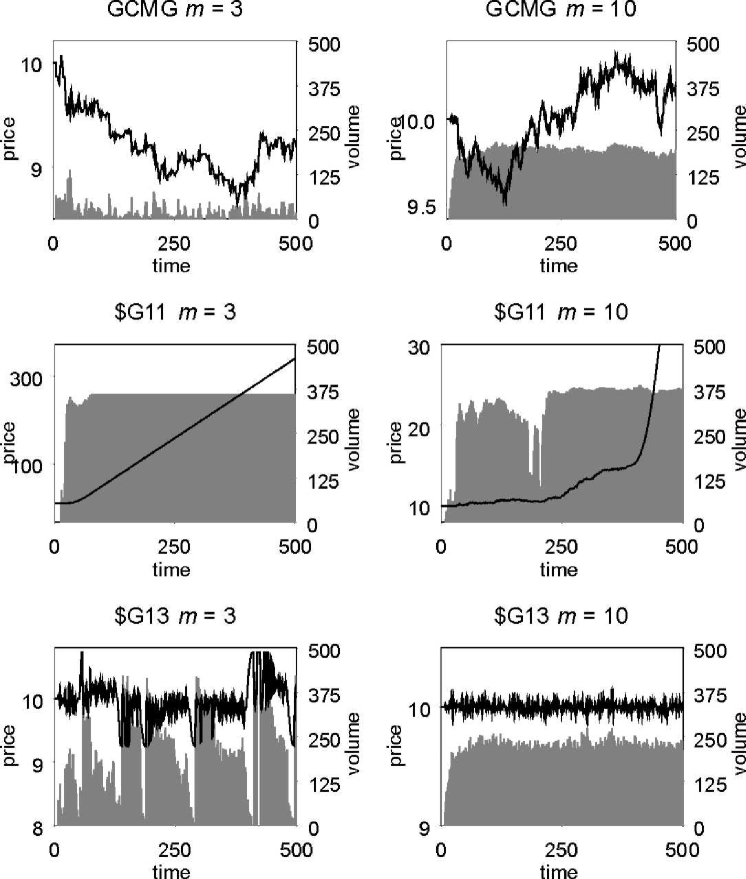
Figure 1: Behaviour of price and volume in market models corresponding to three different strategypayoff functions $g_{R}\left[t\right]$. Parameters for each model are $N=501$, $s=2$, $T=100$, $r=4$. The left hand column represents the crowded market with high agent coordination ($m=3$) the right hand column represents an uncrowded market with little agent coordination ($m=10$). The top row shows the GCMG, the second row shows the $G11 and the bottom row shows $G13.

The two different values of the agent’s memory length (or rather the ratio $P/N$) describe markets in two distinctly different ‘phases’. Arguably the most important feature of these types of model is that there is a common perception of a strategy’s (virtual) success, i.e. $S_{R}\left[t\right]$ is a global variable. This implies that the number of agents adopting the same action (i.e. the effect of crowding or herding) is dependent on the number which hold each strategy. At low memory (low $P/N$) there are few strategies available and many agents, consequently large numbers of agents hold the same strategy. This implies that in this ‘crowded phase’ there are large groups of agents adopting the same action $a_{R}^{\mu\left[t\right]}$ (i.e. crowds) and only small groups adopting the opposite action $-a_{R}^{\mu\left[t\right]}$ (i.e. anti-crowds) [18]. The result of this high agent coordination is a volatile market with large asset price movements. Conversely, for high $m$ (high $P/N$) hardly any agents hold the same strategy. Hence the crowd size is roughly equal to the anti-crowd size, resulting in a market with low agent coordination and consequently lower volatility and fewer large changes. With this distinction between low and high $m$ regimes in mind, let us briefly describe the dynamics in each market model.

• GCMG. First consider low $m$. The confidence-to-play threshold is set high enough in order that occasional stochasticity is injected via timesteps when $A\left[t\right]=0$ (N.B. the next state of $\mu\left[t+1\right]$ is then decided with a coin toss). The GCMG can be seen to reproduce many of the statistical features observed in real markets. Figure 1 shows that the activity (volume) is generally low and bursty. The asset price series is thus characterized by frequent large movements (giving fat-tailed distributions of returns) and clustered volatility. No long periods of correlation exist in the GCMG asset price movement: as soon as lots of agents start taking the same action, then the strategies which produce that action are penalized, as can be seen from Equation 1. At high $m$, the absence of agent co-ordination leads to an absence of clustering of activity. Hence the series of asset prices appears more random at high $m$.

• $G11. At low $m$, the asset price very soon assumes an unstoppable trend: agents with at least one trend-following strategy ($\ldots A\left[t-2\right]>0,A\left[t-1\right]>0,A\left[t\right]>0\Rightarrow a_{R}=1$) join the trend and benefit (notionally) from the consequent asset price movement. Because the strategies (and hence agents) are allowed to accumulate limitless positions, the trend is self-reinforcing since $\Delta W_{R}$ just keeps getting bigger for the trend-following strategies. At high $m$, the lack of agent coordination means that it is harder for the model to find this attractor. However sooner or later, a majority of trend-following strategies will have accumulated sufficient score $S_{R}$ and position $\left|\phi_{R}\right|$ to be played successfully. From then on, the pattern of success is self-reinforcing and again the unstoppable trend is created. This result has to be seen as the natural consequence of wanting the agents to maximize notional wealth at the same time as being allowed arbitrarily large positions.

• $G13. At low $m$, the model has interesting and irregular dynamical properties. For example, the series of asset price movements contains periods of very high correlation (and high volume) and periods of very high anti-correlation (and lower volume). These two behaviors arise from the payoff structure of Equation 13: just as in $G11, strategies are rewarded for having a positive (negative) position when the asset price is trending up (down), however they now get penalized for joining that trend. This implies that persistent behavior will tend to follow persistent behavior, while anti-persistent behavior will follow antipersistent behavior. This finding is very much in line with the school of thought that says that markets have distinct ranging and breakout phases. Unlike the $G11 model, the trends are always capped by the limitation that agents can only hold one position. Once as many agents as possible are long (short) the asset price cannot rise (fall) any further: consequently the resulting dynamics are strongly mean-reverting. At high $m$, due to the lack of agent coordination, it is hard for large enough crowds to arise to form trending periods. Thus anti-persistence dominates this regime.

7 Instability in market models

In the MG, there is no unstable attractor which could give rise to a continuously diverging price. The reason is that each agent is trying to do the opposite of the others. This results in no net long-term market force. The MG agents can see no advantage in collectively forcing a price up (down) to increase the value of their long (short) position, since they are totally unaware of their accumulated position. Section 6 showed however that, when we give the agents the goal of maximizing their notional wealth (cash plus value of position), the model can be dominated by the unstable dynamics of price trending. Although the structure of the $G models seems more realistic than the MG, the price dynamics do not reproduce many of the stylized features of financial asset price series. It seems that an improvement in the microscopic model structure ‘spoils’ the macroscopic results. To help explain this, we now look at some of the model deficiencies which still remain.

7.1 Market impact

We hinted at this effect in Section 4. The wealth $W_{i}\left[t\right]$ that we have forced the agents of the $G models to maximize, is purely notional - it is the wealth they would have if they could unwind their market positions at today’s price $p\left[t\right]$. The agents are clearly not able to do this. There are two reasons for this. Even if an agent put in an order to unwind his position at time $t$, it would not be executed until time $t+1$ when the price is $p\left[t+1\right]$. The second reason is that in this simplistic structure, the agents can only trade one quanta of asset at any time. Hence a position of $\phi_{i}$ assets will take $\phi_{i}$ timesteps to fully unwind. All other things being equal, an agent should expect on average to get less cash back than $\phi_{i}\left[t\right]p\left[t\right]$ when unwinding his position. This is ‘market impact’. We can see this effect directly with the following argument:

The change in cash of agent $i$ from buying $\Delta\phi_{i}\left[t,t-1\right]$ assets at time $t$ is given by: $\Delta C_{i}\left[t,t-1\right]=-\Delta\phi_{i}\left[t,t-1\right]p\left[t\right]$. Let us then use Equation 4 to give $p\left[t\right]=p\left[t-1\right]+D\left[t^{-}\right]/\lambda$. Then we break down the demand as follows:

$$D\left[t^{-}\right]=d_{i}+\sum_{j\neq i}^{N}d_{j}\left[t^{-}\right]$$

where $d_{j}$ is the demand of agent $j$. However we know that the demand of agent $i$ is $\Delta\phi_{i}\left[t,t-1\right]$ assets, hence we get

$$\Delta C_{i}\left[t,t-1\right] =-\Delta\phi_{i}\left[t,t-1\right]p\left[t\right]$$

$$=-\Delta\phi_{i}\left[t,t-1\right]p\left[t-1\right]-\frac{1}{\lambda}\left(\Delta\phi_{i}\left[t,t-1\right]\right)^{2}-\frac{1}{\lambda}\Delta\phi_{i}\left[t,t-1\right]\sum_{j\neq i}^{N}d_{j}\left[t^{-}\right]$$

If we now assume that the remaining agents $j\neq i$ form an effective ‘background’ of random demands $d_{j}$ of zero mean, then averaging over this ‘mean-field’ of agents gives:

$$\left\langle\Delta C_{i}\left[t,t-1\right]\right\rangle_{j}=-\Delta\phi_{i}\left[t,t-1\right]p\left[t-1\right]-\frac{1}{\lambda}\left(\Delta\phi_{i}\left[t,t-1\right]\right)^{2}$$ (14)

Equation 14 tells us that an agent will on average receive an amount of cash $\left\langle\Delta C_{i}\left[t,t-1\right]\right\rangle$, which is equal to the amount he may have naively thought he would get (if he could have traded at price $p\left[t-1\right]$) minus a positive amount proportional to the square of his trade size and inversely proportional to the market liquidity. Consequently, an agent who considered his market impact in calculating his wealth would on average expect the cash-equivalent value of his wealth to be given by $W_{i}\left[t\right]-\phi_{i}\left[t\right]^{2}/\lambda$, i.e. his notional wealth minus the average impact from unwinding his position at time $t+1$. This is the wealth that the agents should be attempting to maximize. We could therefore propose, in the spirit of Ref. [19], a modification to the strategy reward function $g_{R}\left[t\right]$ which takes account of this market impact:

$$g_{R}\left[t+1\right]\varpropto\chi\left[\phi_{R}\left[t\right]\Delta p\left[t+1,t\right]-\phi_{R}\left[t\right]^{2}/\lambda\right]$$ (15)

Let us now re-visit the issue of trend following, this time with reference to a model whose strategies are updated using Equation 15. We will refer to this model as $G15. When a trend forms such that $\phi_{R}\left[t\right]$ and $\Delta p\left[t+1,t\right]$ have the same sign, strategy $R$ will be rewarded: this continues until the moment when the extra profit gained from increasing the position to benefit from the favorable price movement, is smaller than the added market impact which would be faced from unwinding the larger position. At this point the strategy will start to be penalized instead of rewarded for supporting the trend. This is a mechanism which could halt the price-divergent behavior of $G11 type models. However Equation 15 gives the turnover point in strategy reward due to market impact, to be given by $\phi_{R}\left[t\right]=\lambda\Delta P\left[t+1,t\right]$. If we then consider that during an ‘unstable’ market trend the average price change is of order $N/\lambda$ (see, for example, the gradient of the $G11 price in Figure 1) - and that $\phi_{R}$ increments by only $\pm 1$ every timestep - then trends which are formed before the market impact mechanism starts having a strong effect, will be of order $t_{\text{trend}}\backsim N$ timesteps in length. The market impact mechanism on its own, is thus clearly too weak to stabilize the $G models in order to form a realistic price series.

7.2 Agent wealth

Financial agents participating in a real market have finite resources and so cannot keep buying and/or selling assets indefinitely. This hard cut-off of agents’ resources in turn imposes a hard limit on the magnitude of price trends. This effect was seen clearly in the $G13 model where the agents were only permitted (or, equivalently because of finite resources, were only able to) hold one position at any one time. The $G13 and $G11 models can thus be thought of as opposite extremes in this respect, i.e. the first mimics extremely tightly-limited resources while the second mimics infinite resources. It seems natural to expect that a real financial market lies somewhere between these two extremes; resources are large for the market-moving agents but still finite. We can include the effect of limited agent resources in our market model by allocating agent $i$ an initial capital $C_{i}\left[0\right]$ (and position $\phi_{i}\left[0\right]$) and then updating this capital using $C_{i}\left[t\right]=C_{i}\left[t-1\right]-\Delta\phi_{i}\left[t,t-1\right]p\left[t\right]$ [4]. The agents cannot then trade at time $t$ if the following conditions are met:

$$\Delta\phi_{i}\left[t,t-1\right] >0\cap C_{i}\left[t-1\right]<\Delta\phi_{i}\left[t,t-1\right]p\left[t-1\right]$$

$$\Delta\phi_{i}\left[t,t-1\right] <0\cap\phi_{i}\left[t-1\right]<0$$

In other words, an agent will not submit a buy order unless he at least has the capital to buy the asset at the quoted price $p\left[t-1\right]$, and also will not submit an order to short sell if he already holds a short position. If we imposed no limit on short selling, an unstable state of the system would exist wherein all agents short-sell indefinitely.

We will refer to this model as $G11W where W represents ‘wealth’. Let us initialize this market model with agent wealths such that the agents’ initial buying power is equal to their initial selling power, i.e. $\left\{C_{i}\left[0\right],\phi_{i}\left[0\right]\right\}=\left\{n\times p\left[0\right],n-1\right\}.$  Hence initially, the agents have the power to buy or sell $n$ assets (N.B. recall that they are allowed up to one short sell). If we then raise $n$ from $n=1$ upwards, we can see a qualitative change in the dynamical behavior of the model between the two extremes of $G13 and $G11, with the periods of trending growing longer as $n$ increases. To investigate this behavior numerically, we fix $n$ and run the model for 1500 timesteps, recording the value of the global information $\mu\left[t\right]$ in the last 500 timesteps $t$. We then count the number of times within this last 500 timesteps that either $\mu=0$ (implying negative price movements over the last $m$ timesteps) or $\mu=P-1$ (positive price movements) occur. We denote the frequency with which these states occur as $f_{\text{trend}}$. If the model visited all states of the global information $\mu\left[t\right]$ equally, we would expect $f_{\text{trend}}=1/P$. Figure 2, showing the variation of $f_{\text{trend}}$ with $n$, has several interesting features. First it can be seen that, as $n$ is increased and the consequent wealth available to the agents grows, the tendency of the model to be dominated by price trending increases dramatically. Also we see that at low $n$, $f_{\text{trend}}$ is below that of the (random) equally visited $\mu$-states case. This is due to the high degree of anti-persistence in the system as was seen in the $G11 model. The large spread in the results arises from the tendency of the model to exhibit clustering of activity states: persistence follows persistence and anti-persistence follows antipersistence as described in Section 6.

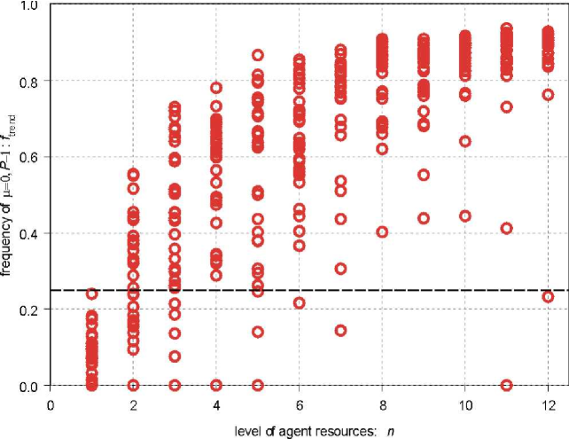
Figure 2: The frequency of occurence of the global information states $\mu=0,P-1$, $f_{\text{trend}}$, as a function of the agents’ capital resource level $n$. The results were taken from the last 500 timesteps of a 1500 timestep simulation. The market model used was $G11W, with evolving agent wealths. The model parameters were $N=501$, $m=3$, $s=2$, $T=100$, and $r=4$, with binary ($\chi=\operatorname*{sgn}$) strategy rewards. The solid line represents equally visited $\mu$-states.

We note that in the work of Giardina and Bouchaud (see Refs. [6, 15]) the strategy payoff function has the same basic form as Eq. 13, i.e. it is a $G13W-style model. These authors consider proportional scoring (i.e. $\chi=1$) and include an interest rate which resembles a resource level $L$; these features will not change the qualitative results presented here. However, in the models of Refs. [6, 15], it seems that only active strategies are rewarded thereby breaking the common perception of a given strategy’s success among agents which is arguably a central feature of the binary model structure. We expect this to dramatically affect the dynamical properties of the system as the mechanism for agent coordination and thus crowd formation has been altered.

7.3 Diversity and timescales

The interesting dynamical behavior of market models based on the binary strategy approach of the MG, arises largely as a consequence of the heterogeneity in the strategies held by the agents and the common perception of a strategy’s success. The extent to which agents will agree on the best course of action, and the consequent crowding, is solely a function of how the $2^{P}$ available strategies are distributed amongst the population of agents. If the way in which the strategies are initially allocated is biased, then the resulting dynamics will reflect this [6].

The introduction of an agent wealth, as discussed in the previous subsection, also brings about diversity in the market model. Even if we initiate the model with all agents having an equal allocation of wealth in the form of cash plus assets, the wealths of the agents $\{W_{i}\}$ will soon become heterogenous as a direct result of their heterogenous strategies. Figure 3 shows the heterogeneity of agents’ wealth growing with time during a $G11W simulation. After many timesteps have elapsed, the distribution of agents’ wealth seems to reach a steady-state: many agents have lost the majority of their wealth to a minority of agents who themselves have accumulated much more. In everyday terminology, ‘the rich get richer while the poor get poorer’.

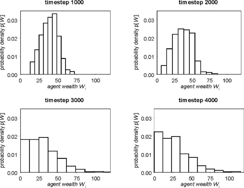
Figure 3: Distributions of the agents’ wealth $W_{i}$ at four different times $t$ during evolution of a $G11W model. Initially all agents were allocated the same resources $\left\{C_{i}\left[0\right],\phi_{i}\left[0\right]\right\}=\left\{3p\left[0\right],2\right\}$ with the initial price $p\left[0\right]=10$. Parameters for the simulation were $N=1001$, $m=3$, $s=2$, $T=100$, and $r=4$, with binary ($\chi=\operatorname*{sgn}$) strategy rewards.

The heterogeneity of agents’ wealth in the $G11W model is fed back into the system through the buying power of the agents alone. However, although wealthier agents have the potential to buy and sell more assets, they still only trade in single quanta of the asset at any given timestep, the same as poorer agents. It may be more reasonable to propose that the agents trade in sizes proportional to their resources [4, 6], i.e.

$$\Delta\phi_{i}\left[t,t-1\right] =\gamma\frac{C_{i}\left[t-1\right]}{p\left[t-1\right]}\text{ \ \ for \ \ }a_{R_{i}^{\ast}}^{\mu\left[t-1\right]}=1$$

$$\Delta\phi_{i}\left[t,t-1\right] =\gamma\phi_{i}\left[t-1\right]\text{ \ \ for \ \ }a_{R_{i}^{\ast}}^{\mu\left[t-1\right]}=-1$$

where $R_{i}^{\ast}$ is the highest scoring strategy $R$ of agent $i$. The factor $\gamma$ then enumerates what fraction of the agents’ resources (cash for buying, assets for selling) they will transact at any given time. In this system, assets will generally need to be divisible, i.e. the sense of agents buying and selling a quanta of the asset as in $G11W is lost. This in turn means that instead of the degree of trending being controlled by the level of initial resource allocation $n$, it is instead determined by $n/\gamma$, since this effectively determines the number of trades agents can make in any trending period before hitting the boundary of their capital resources. Also with this system of trading in proportion to wealth, trends will start steep and end shallow as agents run out of resources and thus make smaller and smaller trades. Apart from these stylized differences, the system has a very similar dynamical behavior to the more straight-forward $G11W model.

Diversity in strategies and wealth are the two big sources of agent heterogeneity that we have covered so far. This agent heterogeneity has led to a market model with dynamical behavior which is interesting and diverse over a large parameter range. However, the typical price/volume output only starts to become representative of a real financial market at higher $m$, as can be seen in Figure 4. As discussed in Section 6, the high $m$ regime represents a ‘dilute’ market where very few traders act in a coordinated fashion. However one would expect that a real financial market is not in a dilute phase at all, since it does have large groups of agents forming crowds which rush to the market together, thereby creating the bursty activity pattern observed empirically. Why then does this model, when pushed into the low $m$ regime, produce endless bubbles of positive and negative speculation as shown in the left-hand panel of Fig. 4. Although a real financial market does show some suggestion of oscillatory bubble formation, it is nowhere near so pronounced and is certainly not on such a short timescale.

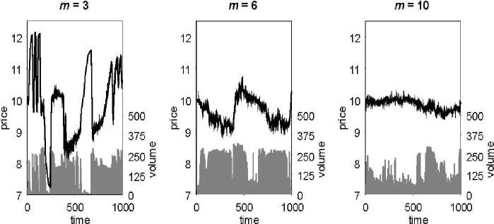
Figure 4: Examples of the dynamical behavior of the price $p\left[t\right]$ and volume $\sum_{i=1}^{N}\left|d_{i}\right|$ of the $G11W model, for three different degrees of crowding given by the memory length $m$. The parameters of the simulation are $N=501$, $s=2$, $T=100$, $r=4$, and $n=3$, with binary ($\chi=\operatorname*{sgn}$) strategy rewards.

To answer this question, we push further the subject of agent diversity. Although our agents may have differing sets of strategies and consequently different wealths, they all act on the same timescale. When we look at charts such as Figure 4, we see patterns not only on a small tick-by-tick scale but also on a much larger scale. In fact we can identify patterns all the way up to the ‘macro’ scale of the boom-bust speculatory bubbles. From a knowledge of these patterns, we would form opinions about what will happen next and would trade accordingly to maximize our wealth. The agents we have modelled, however, cannot view the past price-series in this way; instead they are forced to only consider patterns of length $m$ timesteps. Patterns of any length greater than this, go un-noticed by the agents and hence are not traded upon. This explains why these patterns can arise and survive. By contrast, when a pattern is traded upon (even in the non-MG framework) it is slowly removed from the market. Consider the following pattern:

time $t$	1	2	3	4	5	6	7	8	9	10	11	12	13	14
price $p\left[t\right]$	14	10	11	12	13	15	14	10	11	12	13	15	14	10

If we were able to identify this pattern repeating, our best course of action would be to submit a buy order between times $t=1$ and $t=2$, i.e. $a\left[1\right]=1$. We could then buy the asset at $p\left[2\right]=10$. Then between times $t=5$ and $6$, we would submit an order to sell: $a\left[5\right]=-1$ and hence would have sold the asset at $p\left[6\right]=15$. We then continue: $a\left[7\right]=1$, $a\left[11\right]=-1$… This ensures we always buy at the bottom price and sell at the top. However, trading in this way is against the trend as $a\left[t\right]A\left[t\right]<0$. It is in effect minority trading. Hence trading to maximize our wealth with respect to this pattern, leads to the weakening of the pattern itself just as in the MG. We conclude therefore that the presence of strong patterns in the $G11W and other similar market models at low $m$, is simply due to the absence of agents within the model who can identify these patterns and arbitrage them out.

From the proceeding discussion, it is clear that a realistic market model should include agents who can analyze the past series of asset price movements over different time-scales. A first thought on how to do this, is to include a heterogeneity in the memory length $m$ of the agents. In this framework, agents look at patterns not only of differing length but also of differing complexity. It is therefore appealing to propose a generalization to the way in which the agents interpret the global information of past price movements, in such a way as to allow observation of patterns over different times-scales but having the same complexity ($m$). This can be simply achieved by allowing the agents to have a natural information bit-length $\tau$ such that the global information available to them $\mu_{\tau}\left[t\right]$ is updated according to the following generalization of Equation 7:

$$\mu_{\tau}\left[t+1\right]=2\mu_{\tau}\left[t\right]-P\operatorname{H}\left[\mu_{\tau}\left[t\right]-\frac{P}{2}\right]+\operatorname{H}\left[\Delta P\left[t+1,t+1-\tau\right]\right]$$

The table below then shows how the previous pattern would be encoded by agents having $\tau=1,2,3,4$:

time $t$	$1$	$2$	$3$	$4$	$5$	$6$	$7$	$8$	$9$	$10$	$11$	$12$	$13$	$14$
price $p\left[t\right]$	$14$	$10$	$11$	$12$	$13$	$15$	$14$	$10$	$11$	$12$	$13$	$15$	$14$	$10$
‘best’ action $a^{\ast}\left[t\right]$	$1$	$1$	$1$	$1$	$-1$	$-1$	$1$	$1$	$1$	$1$	$-1$	$-1$	$1$	$1$
$\operatorname*{sgn}\left[\Delta P\left[t,t-1\right]\right]$		$-$	$+$	$+$	$+$	$+$	$-$	$-$	$+$	$+$	$+$	$+$	$-$	$-$
$\operatorname*{sgn}\left[\Delta P\left[t,t-2\right]\right]$			$-$	$+$	$+$	$+$	$+$	$-$	$-$	$+$	$+$	$+$	$+$	$-$
$\operatorname*{sgn}\left[\Delta P\left[t,t-3\right]\right]$				$-$	$+$	$+$	$+$	$-$	$-$	$-$	$+$	$+$	$+$	$-$
$\operatorname*{sgn}\left[\Delta P\left[t,t-4\right]\right]$					$-$	$+$	$+$	$-$	$-$	$-$	$-$	$+$	$+$	$-$

If each agent only considered the past two bits of information, i.e. $m=2$, then the ‘best’ strategies for different values of the information bit-length $\tau$ would be as shown in the table below. These ‘best’ strategies have been obtained from inspection of the table above; in particular, by looking at when the different $m=2$ bitstrings $\left\{--,-+,+-,++\right\}$ occur and seeing the respective ‘best’ action given this bit string $a^{\ast}\left[t\right]$.

	$\tau$
$\mu\left[t\right]$	$1$ $2$ $3$ $4$ $--$ $1$ $1$ $1$ $?$ $-+$ $1$ $1$ $-1$ $-1$ $+-$ $1$ $1$ $1$ $1$ $++$ $?$ $?$ $?$ $1$

The ‘best’ strategies ($\underline{a}_{R^{\ast}}$) in the above table, show a question mark (?) next to a particular value of the global information $\mu\left[t\right]$. This denotes that for this state, the best action is sometimes $a_{R^{\ast}}^{\mu\left[t\right]}=1$ and sometimes $a_{R^{\ast}}^{\mu\left[t\right]}=-1$. It can thus be seen that only when we include longer time-scale patterns $\tau>2$, do we get a clear signal of when is the optimal time to sell ($a_{R^{\ast}}^{\mu\left[t\right]}=-1$). Shorter timeframe patterns provide no clear indication when to do so. This then demonstrates that an agent holding strategies of different bit-length $\tau$ could identify optimal times to buy and sell, and hence arbitrage patterns of length very much greater than the memory length $m$.

7.4 Exogenous information

So far this section has discussed how instabilities and inefficiencies in the model market (as indicated by repeating, un-arbitraged patterns) could be remedied by inclusion of more realistic, sophisticated and diverse strategic agents. However the agents we have considered have all acted in the same fashion, i.e. with the goal of maximizing their wealth by employing a strategic methodology based on the observable endogenous market indicators. In terms of a real financial market, we have considered modelling the subset of agents who consider the past history of asset price movements as the only relevant information. Although in reality we expect this subset to be large, we certainly acknowledge the presence of agents who strategically use other endogenous market indicators such as volume as a source of global information. The strategic use of other endogenous market indicators simply gives a more sophisticated model within the same basic framework.

What we have so far neglected to include is the presence of agents using exogenous information to influence their trading decisions. Possible sources of exogenous information are as vast as human imagination itself: they could for example range from economic indicators through to company reports and rumor, or even ‘gut-feeling’ and astrology! Within the context of our model framework, strategies employed based on these external sources of information are un-strategic with respect to the endogenous information, and as such represent a stochastic influence.

Such stochasticity, representing the response of agents to exogenous information, can be incorporated into the models in a variety of ways. For example a background level of stochastic action could be assumed at each timestep, or be made to appear as a Poisson process with a given mean frequency. However, it seems most physically satisfying to incorporate stochastic action in the form of an extra pair of strategies for each (or at least some) agent: one buy strategy, $\underline{a}_{R}=\underline{1}$, and one sell strategy, $\underline{a}_{R}=-\underline{1}$. Agents could then be given a probability of using each of these strategies in place of their ‘usual’ chartist strategies. Furthermore, the probabilities of using these strategies could be allowed to evolve. This system of modelling response to an exogenous signal is essentially the ‘Genetic Game’ of Ref. [20]. Alternatively, the probability of using one of these strategies representing the response to an exogenous signal, could be based on an endogenous market indicator. An example of this is the mechanism of Ref. [6] of switching to ‘fundamentalist behavior’. In the model of Ref. [6], agents use strategy $\underline{a}_{R}=\underline{\operatorname*{sgn}\left[p_{0}-p\left[t\right]\right]}$ with a probability $f$ which increases with $\left|p\left[t\right]-p_{0}\right|$, where $p_{0}$ represents a perceived ‘fundamental’ value for the asset. This mechanism, which can be thought of as encoding the behavior of irrational fear, clearly acts to break the formation of long trends since the probability of trading against the trend increases with the duration of the trend itself. More generally, we suspect that among the agent-based market models in the literature which manage to reproduce stylized facts, the inclusion of some level of stochasticity within the model is crucial for helping to break up unphysical dynamics and hence achieve market-like behavior.

8 Strategy structure

In the framework of the MG, each strategy $\underline{a}_{R}$ comprises the elements $a_{R}^{\mu}$ which represent a response $\left\{-1,1\right\}$ to each of the possible $P$ values of the global information $\mu$ (see Section 2). In Section 4, we identified the different states of the global information $\mu$ as corresponding to different patterns in the past history of asset price movements (binary: up/down). We can therefore think of a strategy as a book of chartist principles recommending an action for each and every possible pattern of length $m$. Each of these strategy ‘books’ thus has $2^{m}$ pages, one for each pattern. There are $2^{2^{m}}$ possible books an agent can buy and use as guidelines on how to trade. An agent in possession of one of these strategy ‘books’, whichever he chooses to buy, can find a page giving guidelines on how to trade in every possible market state. The books are thus ‘complete’.

It seems unlikely however, that in reality such a ‘complete’ book would exist for any arbitrary value of $m$. Indeed, even if such a book did exist, it is unlikely that a given market participant would consider all the pages as being true. For example, page one of a strategy book may say that if the asset price has fallen three days running, one should sell assets on the fourth day. Page three may say that if the asset price has fallen, then recovered and then fallen again, it is advisable to buy. The agent holding this book may well believe in page one but think that the guidelines of page three are rubbish: in particular, he considers the pattern down-up-down to correspond to no trading signal at all. This agent would therefore continue to hold any previous position he had if he saw the pattern down-up-down. We therefore propose a generalization to the strategy structure of the MG to account for the fact that strategy ‘books’ may be incomplete, or equivalently that agents do not trust some of the trading signals.

Before trading commences, each agent goes through each of her (complete) strategy ‘books’ page by page, and decides whether she believes in the trading guidelines given for each of the possible $P=2^{m}$ market ‘signals’. The agents choose to accept each page of each of their books with a probability $p_{a}$. If the agent rejects a page of the strategy ‘book’, they replace the suggested action for time $t$, i.e. $a_{R}^{\mu\left[t\right]}\in\left[-1,1\right]$, by a null action $a_{R}^{\mu\left[t\right]}=\ast$. When trading commences, the agents are then faced with deciding what course of action to take when their strategy ‘books’ register the null action at time $t$. One type of possible behavior would be to maintain their prior course of action, i.e. $a_{R}^{\mu\left[t\right]}=a_{R}^{\mu\left[t-1\right]}$. Another alternative behavior would be to maintain their prior position, i.e. $\phi_{i}\left[\left(t+1\right)^{-}\right]=\phi_{i}\left[t\right]$. (This results in $a_{R}^{\mu\left[t\right]}=0$ in $G11 type models and $a_{R}^{\mu\left[t\right]}=a_{R}^{\mu\left[t-1\right]}$ in $G13 models).

We now examine the qualitative differences between a model with this incomplete strategy structure, and a model with complete strategies. For this purpose we will assume a GCMG type model, i.e. a model with strategy payoff given by Equation 1. Figure 5 shows the resulting price and volume from two market simulations with incomplete strategies, the probability of non-null action being $p_{a}=0.3$. These are compared with the GCMG which has complete strategies.

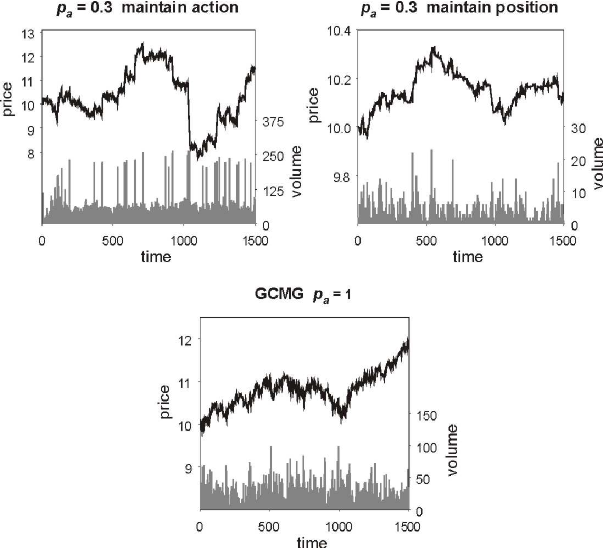
Figure 5: The contrast between the behaviour of models with incomplete strategy ‘books’ to those with complete ones. The top two figures show price and volume for a GCMG type model with incomplete strategies, $p_{a}=0.3$. The top left chart represents a market of agents who maintain their previous action when they encounter a null strategy response $a_{R}^{\mu\left[t\right]}=\ast$. The top right chart represents a market of agents who maintain their position. The bottom chart shows the behavior of the GCMG for comparison. The parameters in all the models are $N=501$, $s=2$, $T=100$, and $r=4$, with binary ($\chi=\operatorname*{sgn}$) strategy rewards.

The top-left chart of Figure 5 shows price and volume for a market where agents maintain their previous course of action when they encounter a null strategy action. This market shows high volatility in price, a high number of very large movements, and a background of high volume trading with occasional sharp spikes. We suggest that this behavior arises from the tendency of agents to keep repeating their previous action in the absence of a new market pattern. Clearly then the ‘large-movement’ states of up-up-up or down-down-down will be occupied for longer than the ‘ranging’ states (up-down-up etc.) because these are the only states of $\mu$ which can map onto themselves ($\mu\left[t\right]=\mu\left[t+1\right]=\mu\left[t+2\right]\ldots$) thus providing no new market pattern.

The top right chart of Figure 5 shows price and volume for a market where agents maintain their previous position (i.e. $a_{R}^{\mu\left[t\right]}=0$ in this model) when they encounter a null strategy action. The volume in this market simulation is very low, giving a consequent low volatility. This is due to the fact that the agents will not trade unless they receive a market signal for which they have a non-null strategy action. This model still shows a high probability for price movements which are large compared to the volatility. These large movements occur in moments of high agent coordination, i.e. when many agents find they have a strategy with the same non-null action. However in contrast to the previous model, these large movements don’t seem to persist over many timesteps.

It is interesting to compare the statistical features of these models featuring incomplete strategies, with the features of the GCMG. Figure 6 shows the volatility and kurtosis of the price movements $\Delta P\left[t+1,t\right]$ for a model with incomplete strategies, as a function of the probability $p_{a}$ that a strategy has a non-null action for a given global information state. The market model used has the structure of the GCMG (N.B. for $p_{a}=1$, it is the GCMG) and features the behavior wherein agents maintain their previous course of action when they encounter a null strategy action. As a consequence, the volatility of the price movements rises as $p_{a}$ is reduced since it leads to more persistence of agent action and consequently bigger asset price movements. This affect can also be seen in the kurtosis which grows rapidly away from the Gaussian case, since the probability of large moves increases with falling $p_{a}$. [For more details on the nature of large movements in the GCMG, we refer to Ref. [21].]

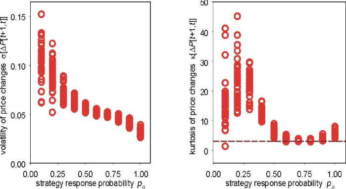
Figure 6: The volatility and kurtosis for a market model with incomplete strategies, as a function of the probability $p_{a}$ that a strategy will have a non-null action for a given global information state. Circles correspond to values taken over the last 1000 timesteps of a 2000 timestep run. The model parameters are $N=501$, $s=2$, $T=100$, and $r=4$, with binary ($\chi=\operatorname*{sgn}$) strategy rewards.

9 Market clearing

In the preceding sections we have discussed mechanisms through which financial market agents come to make trading decisions about whether to buy or sell an asset. In Section 3 we made some suggestions about how the combined action of all these agents’ decisions produced a demand, and how that demand then affected the movement of the asset price. So far we have not explicitly mentioned a mechanism by which the market clears, i.e. by which sellers of the asset meet buyers. The discussion of specific clearing mechanisms amounts to a discussion of specific market microstructure. However our goal here is to seek to be as general as possible, and hence not limit the scope of our market models to any particular sector or style of financial market. We thus limit ourselves here to a simplistic discussion of market-making.

The first important aspect of the models we have considered so far is that the agents make a decision about whether to buy or sell assets at time $t$ based only on the information up to (but not including) time $t$. The orders as such are considered as ‘market orders’ because they are unconditional on the actual traded price $p\left[t\right]$. Orders whose execution depends on the traded price $p\left[t\right]$ are known as ‘limit orders’ and are beyond the scope of the model types presented here.

The presence of only market orders in our model brings us to the second important consideration: the number of buy orders in general does not balance the number of sell orders, i.e. in general $D\left[t\right]\neq 0$ since all orders seek execution at time $t$ irrespective of the price. There are two options then of how the market could function. The first option is to assume that the number of assets sold by the agents must equal the number bought by the agents. In this case the total number of assets traded is given by,

$$v_{\text{assets}}\left[t\right]=\min\left[n_{\text{buy}}\left[t^{-}\right],n_{\text{sell}}\left[t^{-}\right]\right]$$

where $n_{\text{buy}}$ is the number of agents who seek to buy, and $n_{\text{sell}}$ the number who seek to sell. With this system, the agents in the majority group (buyers or sellers) only get their order partially executed: for example if $n_{\text{buy}}=40$ and $n_{\text{sell}}=50$, the sellers can each only sell $v_{\text{assets}}\left[t\right]/n_{\text{sell}}=40/50=80\%$ of a quanta of assets. This is the system proposed in Ref. [6]. An alternative system assumes that there is a third party, a market-maker, who operates between buyers and sellers and makes sure that each and every order is fulfilled by taking a position in the asset herself. We then have that:

$$v_{\text{assets}}\left[t\right]=\max\left[n_{\text{buy}}\left[t^{-}\right],n_{\text{sell}}\left[t^{-}\right]\right]$$

and that the market-maker’s inventory is:

$$\phi_{M}\left[t\right]=\phi_{M}\left[t-1\right]-D\left[t^{-}\right]$$ (16)

The market-maker, unlike the agents who just seek to maximize their wealth, has the joint goals of wealth maximization and staying market-neutral, i.e. as close to $\phi_{M}\left[t\right]=0$ as possible. If the nature of the market is highly mean-reverting, the second of these conditions will be automatically true since $\sum_{j=0}^{t}D\left[t\right]\sim 0$. In these circumstances, the market-maker should employ an arbitrage-free price formation process such as Equation 3 or Equation 4. If on the other hand the market is not mean-reverting, then the market-maker’s position is unbounded. In these circumstances a market-maker should employ a price-formation process such as Equation 5 which encourages mean reversion through manipulation of the asset price based on $\sum_{j=0}^{t}D\left[t\right]$, as described in Section 3. A market-maker using a price formation such as Equation 5 can however be arbitraged by the agents. Whether the market-maker is actually arbitraged is then purely dependent on the underlying dynamics of the market.

Let us demonstrate this by following Ref. [5] using a $G13 model. For this model we have:

$$D\left[t^{-}\right]=A\left[t-1\right]-A\left[t-2\right]$$ (17)

as shown in Section 5. From Equation 16 we then get that $\phi_{M}\left[t\right]=\sum_{j=0}^{t-1}D\left[t\right]=\phi_{M}\left[0\right]-A\left[t-1\right]$ This immediately tells us that the market-maker’s inventory is bounded. The natural choice of price formation process to use would then be the arbitrage-free case of, for example, Equation 3. If we combine Equation 3 with Equation 17 we arrive at:

$$p\left[t\right]=p\left[0\right]e^{\frac{A\left[t-1\right]}{\lambda}}$$ (18)

We can thus see how the $G13 model produced the tightly bounded, jumpy price series seen in Figure 1: the price at time $t$ is no longer directly dependent on the price at time $t-1$ and is bounded by $p\left[0\right]e^{-\frac{N}{\lambda}}\leq p\left[t\right]\leq p\left[0\right]e^{\frac{N}{\lambda}}$.

Given the behavior of the $G13 model, the use of the price formation process of Equation 5 seems rather unnecessary: the market maker does not need to manipulate the price in order to stay market-neutral on average. However, let us demonstrate the effect of using Equation 5 as in Ref. [5]. Combining Equations 5 and 17 with the market maker’s inventory of $\phi_{M}\left[t\right]=-A\left[t-1\right]$ we arrive at:

$$p\left[t\right]=p\left[t-1\right]\exp\left[\frac{1}{\lambda}A\left[t-1\right]+\left(\frac{1}{\lambda_{M}}-\frac{1}{\lambda}\right)A\left[t-2\right]\right]$$ (19)

Unlike Equation 18, Equation 19 gives us again a multiplicative price process for finite values of $\lambda_{M}$. Although it seems an inappropriate step, we would thus expect that introducing Equation 5 as a price formation process would help regain some of the ‘stylized features’ of a financial market inherent from the multiplicative price process. However, closer consideration of Equation 19 reveals something different. Let us consider the case of $A\left[t-2\right]=A\left[t-1\right]$. In this case the price change is simply an increasing function of $A\left[t-1\right]$. If more agents are long rather than short at time $t$ ($A\left[t-1\right]>0$), then the price movement $\Delta P\left[t,t-1\right]$ is positive. The agents will then have benefitted from a positive increment in their notional wealth from simply holding their position. This manipulation of the (naive) market-maker leads to an unstable state whereby the agents arbitrage the market-maker simply by holding their long/short positions and watching the price rise/fall. This unstable state of the market will occur with increasing probability as the agents become more coordinated in their actions, i.e. as $m$ is decreased. For high $m$, where there is no longer significant agent coordination and no crowding affects, the $G13 model with Equation 19 for the price formation is able to avoid the unstable attractor and thus produce more ‘market-like’ time-series as demonstrated in Ref. [5]. We can also examine the changing wealth of the market-maker by simply employing Equation 9. We know that $\phi_{M}\left[t\right]=-A\left[t-1\right]$, so Equation 9 combined with Equation 19 gives us:

$$\Delta W_{M}\left[t+1,t\right] =\phi_{M}\left[t\right]\Delta P\left[t+1,1\right]$$

$$=-\frac{1}{\lambda}A\left[t\right]A\left[t-1\right]-\left(\frac{1}{\lambda_{M}}-\frac{1}{\lambda}\right)A\left[t-1\right]^{2}$$ (20)

In the case of $\lambda_{M}=\lambda$ as in Ref. [5], we see can see - by taking a time average of Equation 20 - that whether the market-maker’s wealth increases or decreases with time will depend on the dynamics of the market. If the market is persistent as in the unstable case at low $m$, the market maker loses wealth since $\left\langle A\left[t\right]A\left[t-1\right]\right\rangle>0$. Conversely if the market is anti-persistent, the market-maker will gain wealth since $\left\langle A\left[t\right]A\left[t-1\right]\right\rangle<0$.

At first sight, it therefore seems that the $G13 model can generate a ‘reasonably market-like’ state wherein the price is not unstable, it exhibits market-like dynamics and has a market-maker who is able to make a profit from her role. However, in order to generate this state it was necessary to use what seems to be an inappropriate market-making mechanism and also push the model into the uncrowded phase. Neither of these choices seem desirable in the quest for producing a realistic market model.

10 Conclusion

Following the introduction to the community of the Minority Game, there have been many proposed agent based market models, many of which exhibit the ‘stylized facts’ of financial market timeseries in certain parameter ranges. It seems however that many of these market models include one or more basic assumptions which seem implausible when compared to the actions of real financial market agents.

With the first ‘wave’ of market models it seemed remarkable that so many of the stylized features of real financial timeseries were reproduced so well. With more and more market model contenders entering the community, each with a quite diverse set of assumptions, it started to look as though it was easy to find models which would reproduce realistic market-like dynamics. It has been proposed [15] that general systems which have activity based on a waiting time problem, will all enjoy the scaling properties seen in financial market data. Notwithstanding this observation, we believe that it is not at all obvious how one can produce a self-consistent market model which embodies, in a non-stochastic way, the behavior of realistic financial market agents, and yet can reproduce the ‘stylized facts’ of real financial markets. As we have shown in this work, adaptation of the MG payoff structure to incorporate a more realistic objective function results in a model increasingly dominated by trending as agents’ resources are increased. As a result of this we are forced to look to a wider class of agent behavior and heterogeneity in order to recover the dynamical behavior we are looking for.

This paper has provided a discussion of different aspects of market models and how they interact with each other. Instead of proposing a unique new market model of our own (thereby adding to the increasing family in the literature), we have examined the different features one may want to include in a market model, and then discussed what their effect would be. We hope that the resulting discussion has managed to provide a basic of toolbox of model features, brought together by a common formalism. Perhaps some optimal combination of a subset of these model features will provide a new self-consistent, realistic yet minimal market model. However it is likely that one needs a diversity not only of agent parameter values but also of agent behavior, if one is intent on forming the market model.

Finally we emphasize that this paper falls into the category of an interim progress report on our research in this area to date - a synthesis of our work over the past few years and thoughts, particularly in light of recent proposals for modified agent-based models. We would therefore welcome any comments and, in particular, criticisms of our results and opinions. We also thank the many people with whom we have enjoyed discussions about financial modelling, both within and outside the Econophysics community.

References

- [1] W.B. Arthur, Science 284, 107 (1999). See also references therein.
- [2] See econophysics website www.unifr.ch/econophysics. See also J. Bouchaud and M. Potters, Theory of Financial Risks (Cambridge University Press, Cambridge, 2000); R. Mantegna and H. Stanley, Econophysics (Cambridge University Press, Cambridge, 2000); B. Huberman, P. Pirolli, J. Pitkow, and R. Lukose, Science 280, 95 (1998); T. Lux and M. Marchesi, Nature 397, 498 (1999); R.G. Palmer, W.B. Arthur, J.H. Holland, B. LeBaron and P. Tayler, Physica D 75, 264 (1994).
- [3] D. Challet and Y.C. Zhang, Physica A 246, 407 (1997); Physica A 256 514 (1998).
- [4] P. Jefferies, N.F. Johnson, M. Hart, and P.M. Hui, Eur. Phys. J. B 20, 493 (2001). This paper was presented at the APFA2 Conference in Liege, 2000.
- [5] J.V. Andersen and D. Sornette, cond-mat/0205423.
- [6] I. Giardiana and J.P. Bouchaud, cond-mat/0206222.
- [7] Sets of past and present working papers can be viewed on the OCCF website www.occf.ox.ac.uk.
- [8] D. Challet, M. Marsili and Y.C. Zhang, Physica A 299, 228 (2001).
- [9] M. Marsili, Physica A 299, 93 (2001).
- [10] J.D. Farmer and S. Joshi, cond-mat/0012419.
- [11] N.F. Johnson, M. Hart, P.M. Hui, and D. Zheng, Int. J. Theo. Appl. Fin. 3, 443 (2000). This paper was presented at the APFA1 Conference in Dublin, 1999.
- [12] N.F. Johnson, P.M. Hui, D. Zheng, and C.W. Tai, Physica A 269, 493 (1999).
- [13] P. Jefferies, D. Lamper and N.F. Johnson, submitted to Physica A (2002). This paper is based on work presented at the APFA3 Conference in London, 2001.
- [14] P. Jefferies, M. Hart, and N.F. Johnson, Phys. Rev. E 65, 016105 (2002).
- [15] I. Giardina, J.P. Bouchaud and M. Mezard, Physica A 299, 28 (2001).
- [16] J.P. Bouchaud and R. Cont, Eur. Phys. J. B 6, 543 (1998); J.D. Farmer, adap-org/9812005.
- [17] T. Chordia, R. Roll and A. Subrahmanyam, in press J. Fin. Econ. (2001); J. Lakonishok, A. Shleifer, R. Thaler and R. Vishny, J. Fin. Econ. 32, 23 (1991); S. Maslov and M. Mills, Physica A 299, 234 (2001); D. Challet and R. Stinchcombe, Physica A 300, 285 (2001).
- [18] M. Hart, P. Jefferies, N.F. Johnson and P. M. Hui, Physica A 298, 537 (2001); N.F. Johnson, M. Hart, and P.M. Hui, Physica A 269, 1 (1999); M. Hart, P. Jefferies, N.F. Johnson, and P. M. Hui, Phys. Rev. E 63, 017102 (2000); N.F. Johnson, P.M. Hui, D. Zheng, and M. Hart, J. Phys. A: Math. Gen. 32, L427 (1999); T.S. Lo, S.W. Lim, P.M. Hui and N.F. Johnson, Physica A 287, 313 (2000); P. Jefferies, M. Hart, N.F. Johnson, and P.M. Hui, J. Phys. A 33, L409 (2000); M. Hart, P. Jefferies, P.M. Hui and N.F. Johnson, Eur. Phys. J. B 20, 547 (2000).
- [19] M. Marsili and D. Challet, cond-mat/0004376.
- [20] N.F. Johnson, P.M. Hui, R. Jonson and T.S. Lo, Phys. Rev. Lett. 82, 3360 (1999); T.S. Lo, P.M. Hui, and N.F. Johnson, Phys. Rev. E 62, 4393 (2000); P.M. Hui, T.S. Lo, and N.F. Johnson, Physica A 288, 451 (2000); N.F. Johnson, D.J.T. Leonard, P.M. Hui, and T.S. Lo, Physica A 283, 568 (2000).
- [21] D. Lamper, S.D. Howison and N.F. Johnson, Phys. Rev. Lett. 88, 017902 (2002).