Statistical properties of one dimensional “turbulence”.

Abstract

We study a one-dimensional discrete analog of the von Kármán flow, widely investigated in turbulence. A lattice of anharmonic oscillators is excited by both ends in order to create a large scale structure in a highly nonlinear medium, in the presence of a dissipative term similar to the viscous term in a fluid. This system shows a striking similarity with a turbulent flow both at local and global scales. The properties of the nonlinear excitations of the lattice provide a partial understanding of this behavior.

1 Introduction

Although studies of turbulence have been carried out for decades, they go on now-days because the problem is very hard and challenging but new ideas have emerged in the last few years from the investigations of statistical properties of turbulence, both at a local or a global scale. First, studies of local longitudinal velocity differences measured at distance $r$ showed that their probability densities are very well described by a theoretical model based on nonextensive statistical mechanics [1], which, in the context of turbulence, can be justified by a phenomenological model based on dynamical foundations [2]. Second, interesting properties showed up in the analysis of the statistical properties of global quantities such as the power consumption of the confined turbulent Von Kármán flow [3] and they culminated with the observation of the universality of rare fluctuations in turbulence and critical phenomena [4].

These recent developments are based on an analysis of experimental results [1, 3]. Indeed only such data contain the full features of turbulence, but for an understanding of the results it would be desirable to have a simple model, showing the basic properties of turbulence, that would be amenable to very detailed studies. The search for simple models of turbulence lead to the introduction of the so-called shell models [5] which describe the energy exchange mechanism between various scales. However shell models are not suitable to study properties that depend on space or to analyze how the dynamics can lead to the observed statistics.

This is why it might be interesting to introduce models of turbulence that are sufficiently simple to allow a detailed study, and nevertheless preserve a spatial structure. In this letter we introduce such a model derived from studies on one-dimensional nonlinear lattices. These systems show various features which are also found in turbulence, and, in particular an exchange of energy between various spatial scales which tends to cause a flow of energy from large scales (long wavelengths) to smaller scales, through the mechanism of modulational instability [6]. The idea to use one-dimensional systems as simple models for turbulence is not new and continuous one-dimensional media have been introduced to study wave turbulence [7], but these studies only lead to weak turbulence. Discrete lattice are attractive for two reasons. First they are simpler since they contain only a limited number of degrees of freedom (and therefore modes), but, more importantly because they have exact localized solutions which could play the role of vortices, the discrete breathers [8], opening the possibility to study an analogous of fully developed turbulence.

Many interesting experimental results on turbulence have been obtained with a simple model flow, the Von Kármán flow produced in the gap between coaxial disks [9]. We investigate here a nonlinear one-dimensional lattice excited by both ends, in a configuration which drives a large scale structure in the system, similar to the vortex of the Von Kármán flow and we show that it exhibits remarkable similarities with turbulence, both for local and global properties.

2 The one-dimensional lattice model.

The system that we study is a one-dimensional chain of anharmonic oscillators, coupled to each other by harmonic interactions. We have chosen Morse oscillators because, the presence of a cubic term in its expansion leads to a suitable nonlinear coupling between the modes, and moreover the lattice of Morse oscillators has localized oscillatory solutions which have interesting properties [10]. In analogy with the Von Kármán flow, we want to drive a finite lattice from both ends, i.e. to inject energy in the system through an external driving. As in actual turbulence experiment where the viscosity of the fluids contributes do dissipate energy, we also need to introduce a dissipation mechanism so that the system can reach a steady state. In analogy with the dissipation term $\nu\nabla^{2}v$ of the Navier Stokes equations, where $\nu$ is the kinematic viscosity, we introduce a dissipation term proportional to the second order finite difference of the velocity of the oscillators, so that the equations of motion of the nonlinear lattice are

$$\ddot{y}_{n}-K(y_{n+1}+y_{n-1}-2y_{n})-2\omega_{0}^{2}e^{-y_{n}}\left(e^{-y_{n}}-1\right)-\nu(\dot{y}_{n+1}+\dot{y}_{n-1}-2\dot{y}_{n})=0\;,$$ (1)

where $y_{n}$ denotes the position of the $n^{\rm th}$ oscillator, $K$ is the coupling constant between neighboring sites, $\omega_{0}^{2}$ determines the depth of the Morse on-site potential, and $\nu$ is a coefficient which plays the role of the kinematic viscosity. As usual, the dot designates a time derivative.

Similarly to the Von Kármán flow where the medium is excited from both ends by a set of rotating disks which create a large scale structure in the system, we consider a finite lattice of $N+2$ particles and we excite it by imposing the displacements of the two end particles, particle $0$ and particle $N+1$. Their motion is chosen according to a linear mode of the lattice, with an amplitude $A$, a wavevector $\kappa=p\pi/(N+3)$, where $1<p<N+1$ is an integer, and a frequency $\omega=\sqrt{2\omega_{0}^{2}+4K\sin\kappa/2}$ (assuming that particles $-1$ and $N+2$ are fixed). Therefore the driving of the system is defined by two parameters, $p$ which fixes its wavevector and frequency and $A$ which determines its amplitude. All simulations start from a lattice at rest and the equations of motion are integrated with a fourth-order Runge-Kutta scheme.

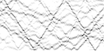
Figure 1: Energy density in a $N=256$-particle lattice excited by a single mode with $p=8$, $A=0.12$. The parameters of the model are $\omega_{0}^{2}=1$, $K=1$, $\nu=5~{}10^{-4}$. The spatial dependence of the energy per unit celle $e_{n}(t)$ is shown with a grey scale (white corresponding to 0 and black to a high energy density). The horizontal axis corresponds to time and extends over a time interval of 20 480 t.u., and the vertical axis gives the position $n$ in the lattice.

Indeed, for such a nonlinear lattice, the fact that the driving corresponds to a single mode of the system does not imply that its response will be merely a single mode. Similarly to the Von Kármán flow, driven by two co-rotating disks, which has a very complex response, the energy density nonlinear lattice also shows a complex spatio-temporal pattern, as displayed in Fig. 1. Localized modes that move in the system, interact with each other, and die out due to dissipation are observed, and they appear to play a role very similar to the vortex filaments in fluids. The point of this study is to observe and analyze the response of the nonlinear lattice to a simple excitation. More complex cases could easily be imagined, such as an excitation with two different frequencies at both ends, which would be similar to some fluid experiments where the two disks have different velocities, but, as shown below the one-frequency driving is sufficient to yield interesting and puzzling results.

3 Local analysis.

Numerical investigations of spatial the Fourier spectrum of the energy density $e(\kappa,t)$ in this simple model have exhibited properties analogous to turbulence, such as a power law spectrum $e(\kappa)=E_{0}\kappa^{\alpha}$ with $\alpha\approx 2.2$ which is remarkably insensitive to the parameters of the model or of the excitation in a very broad range of parameters [11]. When the excitation amplitude increases even more, a transition to a spectrum decaying exponentially versus $\kappa$ is found when the large scale structure created by the excitation breaks down into many smaller scale localized modes, as shown in Fig. 1. This is the regime that we study in this letter. In actual turbulence experiments the energy density cannot be directly measured, but the local velocity is easily accessible. A map of the velocity field would require an array of probes that perturb the flow, and this is why the investigations only evaluate velocity differences measured in 2 points separated by a distance $r$, which provide some information on the spatial structure of the flow, and are also related to the viscous dissipation. For the nonlinear lattice it is easy to calculate an equivalent quantity in the numerical simulations $u(\delta n,t)=\dot{y}_{n_{0}+\delta n}(t)-y_{n_{0}}(t)$, where $n_{0}$ is a fixed reference site and $\delta n$ is an index that measures the distance between the two points, in units of the lattice spacing. It should be stressed that this quantity is local because there is no spatial averaging over the reference site position $n_{0}$.

In a typical numerical experiment, we simulate the dynamics of the system for a time interval of $2~{}10^{7}$ time units (t.u.). The first $5~{}10^{5}$ t.u. are discarded in order to allow the system to reach a steady state before starting the recording of $u(\delta n,t)$. Then we store $u(\delta n,t_{i})$ at times $t_{i}$ separated by an interval $t_{i+1}-t_{i}=40$ t.u. which is large enough to ensure that successive values are statistically independent. This gives us a set of 375000 values $u_{i}$ for each $\delta n$. We evaluate the reduced probability density of this distribution by first calculating $\tilde{u}_{i}=(u_{i}-\langle u_{i}\rangle)/\sigma$ where $\langle\cdot\rangle$ designates a time average and $\sigma=\sqrt{\langle u_{i}^{2}\rangle-\langle u_{i}\rangle^{2}}$ is the variance of the distribution. Then we make a normalized histogram of the $\tilde{u}_{i}$ values in 100 bins to get the normalized probability density $\tilde{P}(\tilde{u})$.

(a)	(b)

Figure 2: (a) Probability density functions of the velocity differences for $\delta n=2$ (top plot) to $\delta n=40$ (bottom plot), by steps of $\delta n=4$. The points correspond to the histograms obtained by numerical simulations and the full lines are the fits of $\tilde{P}(\tilde{u})$ according to Eq. (2). The parameters of the model are $N=256$, $\omega_{0}^{2}=1$, $K=1$, $\nu=10^{-4}$ and $A=0.12$. The reference site is $n_{0}=57$. For better lisibility, each distribution is shifter by -0.5 units. (b) Variations of the fitting parameter $q$ versus $\delta n/\nu$ for different viscosity parameters ($\nu=5~{}10^{-5}$, circles $\nu=1~{}10^{-4}$, stars, $\nu=5~{}10^{-4}$, x, $\nu=2~{}10^{-3}$, squares)

Figure 2a shows such histograms for $\delta n$ varying from $2$ to $40$. The analogy with similar figures deduced form experiments in fluid turbulence is striking (see for instance Fig. 1 in Ref. [1]). The same scenario from almost Gaussian distribution at large distances to stretched distributions at small distances is found. The analogy can be made more quantitative by analyzing the shape of the histograms. The curves of Fig. 2a are very well fitted by the probability distribution deduced from nonextensive statistical mechanics [2, 12]

$$\tilde{P}(\tilde{u})=\frac{1}{Z_{q}}\frac{1}{\left[1+\frac{1}{2}\beta(q-1){\tilde{u}}^{2}\right]^{\frac{1}{q-1}}}\;,$$ (2)

with $\beta=2/(5-3q)$, determined by the condition that the reduced probability distribution should have variance 1. As $Z_{q}$ is a normalization constant, it should be noticed that each curve is fitted with only one free parameter, the parameter $q\geq 1$, which, in the formalism of nonextensive statistical mechanics measures the degree of nonextensivity. With $q\to 1$ ordinary statistical mechanics is recovered and the probability distribution tends to a Gaussian. In the case of turbulence, a formula that generalizes (2) has been derived to take into account the slight skewness of the distributions [2]. The distributions obtained for the nonlinear lattice also have a slight skewness so that the extended formula improves the fit. However, as it is already very good with Eq. (2) we sticked to the expression that minimizes the number of parameters.

The variation of $q$ versus $\delta n$ is shown in Fig. 2b for two values of the viscosity $\nu$ and a mean amplitude $\langle y\rangle\approx 1.1~{}10^{-2}$ in both cases. As for the shape of the probability densities, the similarity with the experimental results on turbulence is strong. At small distances $q$ is significantly larger than 1 ($q\approx 1.3$ in our case) and it decays toward a value close to 1, but above 1, at large distances ($q\approx 1.08$ in our case). In turbulence experiments the variation of $q$ versus distance is essentially determined by the rescaled distance $r/\eta$, where $\eta$ is the Kolmogorov scale which is the typical size of the smallest vortices. In the discrete nonlinear lattice, the size of the smallest breathers is of the order of the lattice spacing, and, in the low viscosity range (high “Reynolds number”) that we are investigating here, it does not vary significantly with the viscosity. This is why $q$ only depends on $\delta n$ for the lattice as shown in Fig. 2b.

4 Global properties of the dynamics.

Our aim in this section is to examine to what extend the one-dimensional nonlinear lattice that we have investigated also shows the same “universal” statistical properties that where observed in critical magnetic systems, self-organized criticality or turbulent flows when one investigate global quantities.

(a)	(b)

Figure 3: a) Probability distribution function (PDF) of the dissipated power $P_{\mathrm{d}iss}$ for different system sizes: from top to bottom $N=256,512,1024,2048,4096$ The parameters of the model are $\omega_{0}^{2}=1$, $K=1$, $\nu=5~{}10^{-5}$. The points correspond to histograms deduced form the numerical simulations and the full lines are fits with the generalized Gumbell distribution. For a better lisibility, each histogram is shifted by -0.5 unit along the vertical axis. b) Variation of the parameter $b$ of the generalized Gumbell distribution versus the system size $N$ in a log-log scale. The error bars correspond to extreme values obtained in different simulations.

In actual turbulence experiments, a global quantity which can be easily evaluated is the power injected by the engines driving the flow, for instance through the disks in the Von Kármán experiment. In the numerical simulations we have however the freedom to evaluate other global quantities directly in the bulk of the system. The power dissipated in the bulk

$$P_{\mathrm{d}iss}=\sum_{n=N/4+1}^{n=3N/4}F_{v}(n)\,\dot{y}_{n}=\nu(\dot{y}_{n+1}+\dot{y}_{n-1}-2\dot{y}_{n})\,\dot{y}_{n}$$ (3)

(where $F_{v}$ is the viscous force) is particularly interesting because it probes the dissipation, an essential physical process for turbulence, at a global scale without being affected by the boundary effects. To avoid any perturbation due to boundaries, we evaluate $P_{\mathrm{d}iss}$ by summing all the dissipative contribution from $n=N/4+1$ to $3N/4$, i.e. in the central half of the system.

As $P_{\mathrm{d}iss}$ is a global quantity, one could think that it would be smooth and featureless due to averaging. This is not the case. In addition to small amplitude fluctuations, the signal shows sharp peaks corresponding to strong bursts of dissipation. This feature shows up on the normalized probability distribution function (PDF) obtained from an histogram of the recorded values of $P_{\mathrm{d}iss}$ in numerical simulations. Figure 3 show such histograms plotted in logarithmic scales as a function of $\theta=(P_{\mathrm{d}iss}-\langle P_{\mathrm{d}iss}\rangle)/\sigma$ where $\langle P_{\mathrm{d}iss}\rangle$ is the time average of the dissipated power and $\sigma_{\mathrm{d}iss}$ its standard deviation. The dissipation bursts give rise to a highly asymmetric PDF with a large tail on the negative side. The dissipation bursts are associated to collisions of the localized excitations, the discrete breathers, that are visible on Fig. 1. Using an approximate expression of the breathers we can evaluate, in the continuum limit, the time average of the power dissipated by a breather. It shows that the dissipation grows with the third power of the breather amplitude, so that the large peaks observed during breather collisions generate strong bursts of dissipation.

Figure 1 showing the space-time evolution of the energy density illustrates a typical situation where one observes localized structures having a long life-time and a complex pattern of interactions. They travel on long distances introducing long range correlations in the dynamics of the lattice. In the context of the general studies of correlated systems which have been performed recently [4], systems showing such correlations have been called “inertial systems” and they display a strongly non Gaussian probability distribution function of some global quantities. As shown by Fig. 3, this is also true for the nonlinear lattice that we investigate here. The strong asymmetry of the PDFs is similar to the observations made on turbulence and critical phenomena [3, 4]. In order to evaluate this quantitatively, we have fitted the numerical PDFs with a generalized Gumbell distribution

$$\Pi(\theta)=w\exp\left[a\left(b\theta-e^{b\theta}\right)\right]\;,$$ (4)

where $w$ is the normalization factor and $a$, $b$ are parameters of the fit. Figure 3 shows that this expression gives a very good fit of the observed distributions, and is able to describe properly their evolution as a function of the system size $N$. In the limit $b\to 0$ the distribution (4) tends to a Gaussian distribution $\Pi(\theta)=w^{\prime}\exp[-\theta^{2}/(2\sigma_{0}^{2})]$ with a standard deviation $\sigma_{0}=1/(ab^{2})$. The value $b=1$ corresponds to the standard Gumbell distribution observed in a turbulent flow [3], and larger values of $b$ correspond to even larger deviations from Gaussianity. Figure 3 shows that, even for large systems ($N=4096$) the fluctuations of $P_{\mathrm{d}iss}$ stay highly non Gaussian.

The origin of this non-Gaussian behavior can be understood from the same argument as for the case of turbulence or critical phenomena [4]: there are long range correlations in the system which cannot be divided into statistically independent regions. However the origin of these long range correlations appears to be different. While in the vicinity of a phase transition correlations are due to the existence of structures at all scales, in the present case, we observe small scale structures (localized modes) which can move on long distances and preserve their identities in collisions (see Fig. 1). However the localized modes are not solitons and are therefore perturbed by the collisions, which limits the correlations to a finite range. As a result the PDF of the dissipated power depends on the size of the system and on the density of localized modes, both of which determine the average number of collisions that a localized excitation experiences when it travels inside the part of the lattice in which we compute the dissipated power (i.e. along $N/2$ sites).

The effect of the size of the system is shown in Fig. 3b which shows that $b$ decreases with $N$ approximately with a power law $b\propto N^{-0.67}$ for $128\leq N\leq 4096$ so that the approach of a Gaussian distribution for large systems is very slow. The study of the effect of the mean amplitude of the displacement, which is correlated to the density of localized modes in the system, shows that a strong non-Gaussianity of the power dissipated in the system persists for variations of $\langle y\rangle$ that extend on more than two orders of magnitude.

Consequently, contrary to the case of turbulence where a universal form of the fluctuations of a global quantity, independent of the Reynolds number, was found [3], the shape of the PDF of the power dissipated in the nonlinear lattice changes with the size of the system or amplitude of the excitation. However it stays strongly non-Gaussian and well described by a generalized Gumbell distribution for all the cases that we could investigate. One may wonder what are the differences between the turbulent flow and our model system. One possibility is the existence in the turbulent flow of structures at all scales, including the integral scale, i.e. flow patterns that have a characteristic size equal to the size of the system, which is not true for the nonlinear lattice. One may ask however whether larger Reynolds number would not break the large vortex into smaller filaments, leading to a gradual change in the shape of the PDF. Such a regime, if it exists, is probably beyond experimental possibilities, while, for the one-dimensional nonlinear lattice, the simulation can examine a very broad range of dynamical behaviors.

5 Conclusion

In this work we examined a simple model related to turbulence. The statistics of its local and global properties are remarkably similar to the experimental results of actual turbulence so that it could be useful for its understanding because it is sufficiently simple to allow detailed studies and test ideas. The remarkable features of the local and global properties could perhaps be understood in a single framework. Global properties of turbulence have been analyzed by Bramwell et al. [4] by pointing out that the flow cannot be divided into mesoscopic regions which are statistically independent. Such a “long range interaction” is precisely what leads to non-extensive thermodynamics [13] which models so well the local properties.

Acknowledgements.

Part of this work has been supported by the EU Contract No. HPRN-CT-1999-00163 (LOCNET network). M.P. wants to thank T. Dauxois and B. Castaing (ENS Lyon) for helpful discussions and E.D.G. Cohen (Rockefeller University) for an illuminating lecture that motivated part of this work.

References

- [1] C. Beck, G. S. Lewis, H. L. Swinney, Phys. Rev. E 63 035303(R) (2001)
- [2] C. Beck, Physica A 277, 115 (2000)
- [3] J.F. Pinton P.C.W. Holdsworth, and R. Labbé, Phys. Rev. E 60, R2452-R2455 (1999)
- [4] S.T. Bramwell, P.C.W. Holdsworth and J.F. Pinton, Nature 396, 552-554 (1998) and S.T. Bramwell, K. Christensen, J.-Y. Fortin, P.C.W. Holdsworth, H.J. Jensen, S. Lise, J.M. López, M. Nicodemi, J.F. Pinton and M. Sellitto, Phys. Rev. Lett. 84, 3744-3747 (2000)
- [5] I. Daumont, T. Dombre and J.L. Gilson, Phys. Rev. E 62, 3592-3610 (2000). For in introduction to shell models, see T. Bohr, M.H. Jensen, G. Paladin and A. Vulpiani Dynamical systems approach to turbulence and extended systems (Cambridge University Press, Cambridge, 1998)
- [6] Y.S. Kivshar and M. Peyrard, Phys. Rev. A 46, 3198-3205 (1992) and I. Daumont, T. Dauxois and M. Peyrard, Nonlinearity 10, 617-630 (1997)
- [7] A.I. D’yachenko, V.E. Zakharov, A.N. Pushkarev, V.F. Shvets and V.V. Yan’kov Sov. Phys. JETP 69 (6) 1144-1147 (1989)
- [8] R.S. MacKay and S. Aubry, Nonlinearity 7, 1623-1643 (1994)
- [9] P.J. Zandberg and D. Dijkstra, Ann. Rev. Fluid Mech. 19, 465-491 (1987)
- [10] T. Dauxois and M. Peyrard Phys. Rev. Lett. 70 3935-3938 (1993)
- [11] I. Daumont and M. Peyrard, unpublished.
- [12] C. Beck, Phys. Rev. Lett. 87, 180601-1-4 (2001)
- [13] C. Tsallis, J. Stat. Phys. 52, 479 (1988)