Multistable transport regimes and conformational changes in molecular quantum dots

Abstract

We analyse non-equilibrium transport properties of a single-state molecular quantum dot coupled to a local phonon and contacted by two electrodes. We derive the effective non-equilibrium (Keldysh) action for the phonon mode and study the structure of the saddle points, which turn out to be symmetric with respect to time inversion. Above a critical electron-phonon coupling $\lambda_{c}$ the effective potential for the phonon mode develops two minima in the equilibrium and three minima in the case of a finite bias voltage. For strongly interacting Luttinger liquid leads $\lambda_{c}=0$. Some implications for transport experiments on molecular quantum dots are discussed.

Recently the progress in engineering and production of nanoscopic electronic devices reached a new summit as experimentalists reported successful contacting of single molecules thereby opening the way to build molecular quantum dots Park et al. (2000); Reichert et al. (2002). Since bistable FET-based elements play the most important role in modern microelectronics a fabrication of such devices on a nanometre scale would be a natural way of further progress. The molecules involved in the electron tunnelling process naturally possess elastic degrees of freedom which are bound to respond to the applied bias voltage in some way; this has been dubbed – ‘conformational change’ (see e.g. Emberly and Kirczenow (2001)). There have been numerous studies of similar systems Wingreen and Meir (1994); König et al. (1996) though none of them has, to our knowledge, concentrated on the behaviour of the internal degrees of freedom in the relevant non-perturbative, non-equilibrium regime.

To understand the basic physics of the conformational change, in this Letter we ignore all the mindboggling complexity of real molecular dots Kornilovitch et al. (2002) and employ the simplest possible Holstein–type model with a single phonon mode Holstein (1959). We study how this phonon responds to the non-equilibrium electron environment. If one applied a ‘maximum entropy’ principle (such as would be invoked to explain the time-reversal breaking in driven macroscopic systems), one might expect that the molecule would deform is such a way as to facilitate the current flow. By developing the full non-equilibrium theory we shall show that such scenario, while admissible in principle, is not correct for the quantum system in question. Instead we find that in this case a generalised non-equilibrium free energy is being minimised and multistable transport regimes emerge.

Figure 1: Schematic representation of the system under investigation. A single quantum dot level $d$ coupled to a local boson mode $Q$ can be populated via tunnelling from two fermionic reservoirs $\psi_{1}$ and $\psi_{2}$. The latter are kept at a fixed chemical potential difference $V$. The gate voltage $V_{G}$ enables controlling of the dot level population.

Let us begin with the Hamiltonian of the system,

$$H=H_{0}[\psi_{1}]+H_{0}[\psi_{2}]+H_{Q}+(\Delta+\lambda Q)d^{\dagger}d+H_{t}\,.$$ (1)

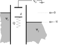
The first two terms on the rhs describe non-interacting Fermi seas in the left and right electrodes; $\psi_{1}$, $\mu_{1}=0$ and $\psi_{2}$, $\mu_{2}=-V$ are the corresponding electron annihilation operators and chemical potentials, $V$ is the bias voltage, see Fig. 1. The third term describes the phonon mode , $H_{Q}=(M\dot{Q}^{2}+KQ^{2})/2$, where $K$ is the elastic constant and $M$ is the oscillator’s mass. The quantum dot is described by the fourth term and contains only one electronic state, which annihilation and creation operators are denoted by $d$ and $d^{\dagger}$, respectively. It can be occupied only by one electron (the spin effects are unimportant as long as the Hubbard coupling is weak so that the system does not enter the Kondo regime, which we assume throughout), which is coupled with a coupling constant $\lambda$ to the local phonon mode $Q$ and has the offset energy $\Delta$. The latter can be controlled by changing the gate voltage $V_{G}$, see Fig. 1. The last term is responsible for the transport through the dot and reads $H_{t}=\gamma[d^{\dagger}(\psi_{1}+\psi_{2})+{\rm H.c.}]$, where $\gamma$ is the energy independent tunnelling amplitude (we assume that the leads are symmetric to simplify formulas).

In most cases the molecular vibrational modes are slower then the electronic degrees of freedom so that it is possible to work in the Born-Oppenheimer (or static) approximation. Within this approximation the instant value of the current is given by:

$$I=\frac{e^{2}\gamma^{2}}{2\pi}\left[\tan^{-1}\left(\frac{\Delta+\lambda Q}{\Gamma}\right)-\tan^{-1}\left(\frac{\Delta+\lambda Q-V}{\Gamma}\right)\right]\,,$$ (2)

where $\Gamma=2\pi\gamma^{2}\rho_{0}$ is the resonance width ($\rho_{0}$ being the local electron density of states). Outside the static approximation, the phonon coordinate $Q$ still possesses its own dynamics. Our goal is to derive the effective action for $Q$. The obvious way to proceed is to eliminate the leads and dot variables in the functional integral representation. Since we are interested in the non-equilibrium situation, we work in the Keldysh representation, where all time integrations are performed along a closed path $C$ which consists of the time-ordered branch $C_{-}$ and the ani-time ordered branch $C_{+}$ Keldysh (1964). Generalising the procedure of Ref. Yu and Anderson (1983), we define the functional,

$$Z[Q]=\langle T_{C}e^{-i\lambda\int_{C}dtQ(t)d^{\dagger}(t)d(t)}\rangle\,,$$ (3)

where $T_{C}$ stands for the contour ordering operation and the average is taken over the exact eigenstate (the steady state) of Hamiltonian (1) with $Q=0$. We set $\Delta=0$ (it will be restored later) and divide the field $Q$ into two Keldysh components scaled by $\lambda$: $Q_{\mp}=\lambda Q(t~{}\mbox{on}~{}C_{\mp})$. The effective action is then $S[Q_{\mp}]=S_{0}[Q_{\mp}]+i\ln Z[Q_{\mp}]$, $S_{0}[Q_{\mp}]$ will be specified shortly. One way to calculate the effective action is to take the functional derivative of $Z[Q_{\mp}]$ respect to, e.g., $Q_{-}$:

$$\frac{\delta Z}{\delta Q_{-}}=-i\langle T_{C}d(t_{-}+0^{+})d^{\dagger}(t_{-})e^{-i\lambda\int_{C}dtQ(t)d^{\dagger}(t)d(t)}\rangle\,,$$ (4)

$t_{-}$ lies on $C_{-}$. If both sides of this equation are divided by $Z$ in order to cancel disconnected diagrams introduced by $Q_{-}$ being different from $Q_{+}$, then the rhs becomes the time-ordered Green’s function of the dot level calculated in the presence of $Q_{\mp}(t)$,

$$D^{--}(t,t^{\prime})=-i\langle Td(t)d^{\dagger}(t^{\prime})\rangle\,.$$ (5)

We now implement the non-equilibrium generalisation of the standard Born-Oppenheimer approximation by calculating the above function (i.e. the electronic response to the phonon) for static time-independent (but different) $Q_{\mp}$, restoring the time dependence at the end of calculation. By means of fermionic functional integration or via the method of Ref. Caroli et al. (1971) we therefore obtain:

$$D^{--}(\omega)=\left\{\begin{array}[]{rr}\frac{\omega-Q_{-}-i\gamma^{2}\mbox{\small sign}\omega}{(\omega-Q_{-})^{2}+\Gamma^{2}}\,;&\omega>0\,\mbox{and}\,\omega<-V\\ \\ \frac{\omega-Q_{+}}{(\omega-Q_{-})(\omega-Q_{+})+\Gamma^{2}}\,;&-V<\omega<0\end{array}\right.\;.\;$$ (9)

Combining Eqs. (4) and (5), one arrives at the following expression for the $Z$-functional:

$$\ln Z/Z_{0}=-\int dt\int_{0}^{Q_{-}}dQ_{-}\int\frac{d\omega}{2\pi}D^{--}(\omega)e^{i\omega 0^{+}}$$

$$+F(Q_{+})\,,$$ (10)

where $F(Q_{+})$ is a yet unknown function depending only on $Q_{+}$ and the explicit time-dependence of $Q_{\mp}$ has now been restored. This procedure results in the loss of non-local in time, dissipative terms, see Ref.Yu and Anderson (1983), which are accessible via perturbative expansions or a generalised Wiener-Hopf method. Such terms are only important for tunnelling between different molecular configurations and will be addressed in the long version Komnik and Gogolin (2002). In the above $Z_{0}$ is responsible for the dynamics of the bosonic mode without the electron-phonon coupling and is given by the functional integral

$$Z_{0}=\int{\cal D}Q_{-}{\cal D}Q_{+}e^{iS_{0}[Q_{\mp}]}\,,$$ (11)

with the free action

$$S_{0}[Q_{\mp}]=\frac{1}{2\lambda^{2}}\int dt\Big{[}M(\dot{Q}_{-}^{2}-\dot{Q}_{+}^{2})-K(Q_{-}^{2}-Q_{+}^{2})\Big{]}\,.$$ (12)

The energy integration in Eq. (Multistable transport regimes and conformational changes in molecular quantum dots) results in two contributions:

$$\ln Z/Z_{0}=-i\int dt\int_{0}^{Q-}dQ[n_{d}(Q) + if(Q,Q_{+})]$$ (13)

$$+ F(Q_{+})\,.$$

The first contribution is purely imaginary and is related to the occupation probability of the dot level,

$$n_{d}(Q)=\frac{1}{2\pi}\Big{[}\cot^{-1}(Q/\Gamma)+\cot^{-1}((Q-V)/\Gamma)\Big{]}\,.$$ (14)

The second contribution is real and is given by

$$f(Q_{-},Q_{+})=\int_{-V}^{0}\frac{d\omega}{2\pi}\Big{[}\frac{\omega-Q_{+}}{(\omega-Q_{-})(\omega-Q_{+})+\Gamma^{2}}$$

$$-\frac{\omega-Q_{-}}{(\omega-Q_{-})^{2}+\Gamma^{2}}\Big{]}\,.$$ (15)

Performing analogous computation the field $Q_{+}$ (or on symmetry grounds), one identifies the missing function as

$$F(Q_{+})=-\int^{Q_{+}}_{0}dQ[n_{d}(Q)+if(Q,0)]\,.$$ (16)

Hence the effective action:

$$S = S_{0}-i\int dt\Big{\{}\int_{0}^{Q_{-}}dQ[n_{d}(Q)+if(Q,Q_{+})]$$ (17)

$$- \int_{0}^{Q_{+}}dQ[n_{d}(Q)+if(Q,0)]\Big{\}}\,.$$

The next step is to minimise the action, which yields the system of coupled equations ($\eta=\pm$):

$$KQ_{\eta}/\lambda^{2}+n_{d}(Q_{\eta})-i\eta f(Q_{\eta},Q_{-\eta})=0\,.$$ (18)

Let us discuss a special class of solutions which satisfy $Q=Q_{-}=Q_{+}$. Function (Multistable transport regimes and conformational changes in molecular quantum dots) vanishes in this case, so all these solutions are real and satisfy the following equation (we restored the energy offset $\Delta$ of the dot level)

$$-KQ/\lambda^{2}=n_{d}(Q+\Delta)\,.$$ (19)

We set $V=0$ first. It is easy to see that for $\Delta<0$ and $\Delta\gg 1/K$ there is only one solution of this equation, see Fig. 2.

Figure 2: Effective potential energy of the phonon as a function of $Q/\Gamma$ for three different gate voltages corresponding to $\Delta/\Gamma=0$, $50$, $100$ (dotted, solid and dashed lines, respectively). In the inset: the graphical solution of Eq. (19). The straight line represents the lhs with $K\Gamma/\lambda^{2}=1$. The curves show the behaviour of the $n_{d}$ (rhs of Eq. (19)) for the same $\Delta/\Gamma$ as in the main graph.

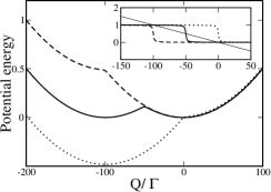
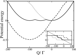
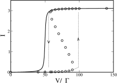
The former situation corresponds to the dot level being placed below the Fermi edges of the leads. In this case the equilibrium position of the phonon mode lies below the Fermi energy. For large and positive gate voltage $\Delta\gg\lambda^{2}/K$ the dot level is effectively attracted by the Fermi sea and the dot energy level is slightly lowered. Unless the slope of the rhs of Eq. (19) at $Q=0$ is smaller than $-K/\lambda^{2}$, which corresponds to $\pi K/\lambda^{2}>\Gamma^{-1}$, there is a third regime when the line $-KQ/\lambda^{2}$ crosses $n_{d}(Q+\Delta)$ three times. In this case the effective potential for the boson mode acquires two dips, see Fig. 2, and the system becomes bistable. A similar bistability in a different (negative-$U$) dot model has recently been reported in Ref.Alexandrov et al. (2002). The non-equilibrium case is even richer. The population probability $n_{d}$ now possesses two steps as a function of energy. This opens the way to tristable regimes as Eq. (19) can have five solutions, see Fig. 3. As in the equilibrium situation multiple solutions are only possible for sufficiently strong electron-phonon coupling, $\pi K/\lambda^{2}<\Gamma^{-1}$. Remarkably, the bistability phenomenon should be visible in the non-equilibrium transport even without any adjustments of the gate voltage. Starting from the equilibrium system with $\Delta=0$ and increasing the bias voltage, see Fig. 4, one inevitably crosses the bistability regime, which reveals itself as a hysteresis in the $I-V$ diagram.

Figure 3: Plot similar to Fig. 2 but for the non-equilibrium case with bias voltage $V/\Gamma=50$. The dashed, solid and dotted lines correspond to $\Delta/\Gamma=0$, $75$, $140$, respectively. The inset shows the graphical solution of Eq. (19) for the non-equilibrium situation.

Figure 4: Current-voltage diagram of a dot with zero offset $\Delta=0$ as a function of the applied bias voltage $V$ (circles). The current $I$ is calculated via Eq. (2) after solving the Eq. (19) and is normalised to $e^{2}\gamma^{2}/2\pi$. The dotted lines represent the actual behaviour of the current whereas circles in between them are the unstable solutions of the Eq. (19). For comparison: solid line is the $I-V$ characteristics of a free dot ($\lambda=0$) with a finite offset $\Delta/\Gamma=50$, $K\Gamma/\lambda^{2}=1$.

For $Q_{-}=Q_{+}$, the correction to the effective action, (17), can be interpreted as an effective non-equilibrium free energy of the phonon mode. We looked for but could not find time-inversion breaking minima with $Q_{-}\neq Q_{+}$. Thus we can confirm that for the system under consideration the ‘quantum Onsager reciprocity principle’, put forward in Ref. Coleman and Mao (2002), is correct. We stress that the Keldysh action approach does not require any external conjectures to hold and allows, at least in principle, for solutions with $Q_{-}\neq Q_{+}$, which would be at odds with Ref. Coleman and Mao (2002). Also, even around the time-invertion symmetric minima, the (slow) phonon dynamics involves fluctuations of two independent but coupled fields $Q_{\mp}$. (In equilibrium all these complications disappear as $Q_{\mp}$ are then simply decoupled.)

With applications to (single-wall) carbon nanotubes in mind, we now briefly discuss the case of interacting leads (in equilibrium). The adequate description in low-energy sector is then given by the Luttinger liquid (LL) model Haldane (1981); Gogolin et al. (1998). To describe the leads we employ the open boundary bosonization procedure. In this approach the electrons can be thought of as chiral particles living on the whole real axis. The tunnelling onto and from the dot level takes place at $x=0$ in both leads. The Hamiltonian has the simplest form in terms of the Bose fields $\phi_{1,2}$ which describe the collective low-density plasmon excitations in the corresponding leads,

$$H_{0}=H_{0}[\psi_{1}]+H_{0}[\psi_{2}]=\frac{1}{4\pi}\int dx\left[(\partial_{x}\phi_{1})^{2}+(\partial_{x}\phi_{2})^{2}\right]\,.$$

The local (at $x=0$) field operators in this representation are then given by Gogolin et al. (1998),

$$\psi_{i}(t)=(2\pi a_{0})^{-1/2}e^{i\phi_{i}(t)/\sqrt{g}}\,.$$ (20)

This equation contains the Luttinger liquid parameter $g$, which is related to the interaction strength $U_{0}$ via $g=(1+4U_{0}/\pi)^{-1/2}$ Haldane (1981), and the lattice constant of the underlying lattice model $a_{0}$. As a next step we substitute (20) into (1) and re-write the dot level operators in terms of spin-1/2 operators, $S_{y}=-i(d^{\dagger}-d)/2$, $S_{z}=d^{\dagger}d-1/2$. After applying a canonical transformation, $U=\exp[iS_{z}(\phi_{1}(0)+\phi_{2}(0))/2\sqrt{g}]$, to the Hamiltonian of the system, $H^{\prime}=U^{\dagger}HU$, and introducing new fields $\phi_{\pm}=(\phi_{1}\pm\phi_{2})/\sqrt{2}$ we arrive at the following Hamiltonian:

$$H^{\prime}=H_{0}[\phi_{\pm}] + QS_{z}-i\gamma\sqrt{2/\pi a_{0}}S_{y}\cos[\phi_{-}(0)/\sqrt{2g}]$$ (21)

$$- \nu\sqrt{2/g}S_{z}\partial_{x}\phi_{+}(0)\,,$$

where we introduced an additional coupling constant $\nu$. Transformed into this form the Hamiltonian is closely related to the Kondo problem . The field $Q$, which is assumed to be adiabatically slow in comparison to electronic degrees of freedom, plays the role of the magnetic field applied to the localised spin $\vec{S}$. The population probability $n_{d}$ is now related to the magnetisation $n_{d}=\langle S_{z}\rangle+1/2$. Correspondingly, the magnetic susceptibility gives us the derivative of the $n_{d}$ with respect to the boson coordinate $Q$.

The special point $\nu=0$ is analogous to the Toulouse limit in the Kondo problem. Moreover, at $g=1/3$ the Hamiltonian coincides with that of the four-channel Kondo problem, see Ref. Gogolin et al. (1998). In order to analyse the magnetic susceptibility we proceed along the lines of Ref. Gogolin et al. (1998). The large time asymptotics of the spin-spin correlation function turns out to be $\langle TS_{z}(t)S_{z}(0)\rangle=Ct^{-2g}$, $C$ being a numerical non-universal constant. Therefore the temperature (and hence energy) dependence of the magnetic susceptibility $\chi=dn_{d}/dQ$ is (after the appropriate continuation to imaginary time):

$$\chi=C^{2}\int_{0}^{1/T}d\tau\langle S_{z}(\tau)S_{z}(0)\rangle\sim C_{1}\,T^{2g-1}\,,$$ (22)

where $T$ is the temperature and $C_{1}$ is another non-universal constant. The last formula has very important consequences for the existence of multistable regimes. In the case of strongly interacting electrodes, when $g<1/2$, $\chi$ is divergent and the slope of $n_{d}$ is infinite. Hence the multistable regimes are always possible when the gate voltage is adjusted in appropriate way and there is no critical electron-phonon coupling. However, $\chi$ vanishes as the temperature or the relevant energy scale approaches zero for weak interactions in the leads, for $g>1/2$. So, for all $1/2<g<1$ there is a threshold in $\lambda$ above which the multistable regimes emerge.

To conclude, we have investigated transport properties of a quantum dot containing one level coupled to a local phonon mode. In the case of non-interacting leads we derived the effective action for the phonon, the analysis of which reveals the existence of a bistable regime in the equilibrium and a tristable regime for finite bias voltage. For strongly interacting leads, the conditions on the electron-phonon coupling needed to enter multistable regimes are relaxed. One obvious avenue for further research is the phonon dynamics close to the bistability where the dissipation rate changes from Ohmic to super-Ohmic at finite bias voltage Komnik and Gogolin (2002). The bulk interaction effects merit further investigation (so, the $g=1/2$ model is exactly solvable by re-fermionization, even at finite $V$.) The most interesting emerging theoretical question is about the viability of time-inversion breaking solutions in similar systems, this question is currently open.

This work was partly supported by the EPSRC of the UK under grants GR/N19359 and GR/R70309 and the EC training network DIENOW.

References

- Park et al. (2000) H. Park, J. Park, A. K. L. Lim, et al., Nature 407, 57 (2000).
- Reichert et al. (2002) J. Reichert, R. Ochs, D. Beckmann, H. B. Weber, M. Mayor, and H. v. Loehneysen, Phys. Rev. Lett. 88, 176804 (2002).
- Emberly and Kirczenow (2001) E. Emberly and G. Kirczenow, Phys. Rev. B 64, 125318 (2001).
- Wingreen and Meir (1994) N. S. Wingreen and Y. Meir, Phys. Rev. B 49, 11040 (1994).
- König et al. (1996) J. König, J. Schmid, H. Schoeller, and G. Schön, Phys. Rev. B 54, 16820 (1996).
- Kornilovitch et al. (2002) P. E. Kornilovitch, A. Bratkovsky, and R. S. Williams, cond-mat/0206495 (2002).
- Holstein (1959) T. Holstein, Ann. Phys., NY 8, 343 (1959).
- Keldysh (1964) L. V. Keldysh, Zh. Eksp. Teor. Fiz. 47, 1515 (1964).
- Yu and Anderson (1983) C. C. Yu and P. W. Anderson, Phys. Rev. B 29, 6165 (1983).
- Caroli et al. (1971) C. Caroli, R. Combescot, P. Nozieres, and D. Saint-James, J. Phys. C 4, 916 (1971).
- Komnik and Gogolin (2002) A. Komnik and A. O. Gogolin, [unpublished] (2002).
- Alexandrov et al. (2002) A. S. Alexandrov, A. M. Bratkovsky, and R. S. Williams, cond-mat/0204387 (2002).
- Coleman and Mao (2002) P. Coleman and W. Mao, cond-mat/0205004 (2002).
- Haldane (1981) F. D. M. Haldane, J. Phys. C: Solid State Phys. 14, 2585 (1981).
- Gogolin et al. (1998) A. O. Gogolin, A. A. Nersesyan, and A. M. Tsvelik, Bosonization and Strongly Correlated Systems (Cambridge University Press, 1998).
- Furusaki and Matveev (2002) A. Furusaki and K. A. Matveev, Phys. Rev. Lett. 88, 226404 (2002).