[

Locally critical point in an anisotropic Kondo lattice

Abstract

We report the first numerical identification of a locally quantum critical point, at which the criticality of the local Kondo physics is embedded in that associated with a magnetic ordering. We are able to numerically access the quantum critical behavior by focusing on a Kondo-lattice model with Ising anisotropy. We also establish that the critical exponent for the ${\bf q}-$dependent dynamical spin susceptibility is fractional and compares well with the experimental value for heavy fermions.

]

How to properly describe heavy fermion metals near quantum critical points (QCPs) is a subject of intensive current research. It is well established experimentally [1] that these systems are prototypes of non-Fermi liquid metals[2, 3]. In a number of cases, striking deviations from the commonly applied $T=0$ spin-density-wave picture (usually referred to as the Hertz-Millis picture)  [4] have been seen. In particular, experiments[5, 6, 7, 8, 9] have shown that the spin dynamics in the quantum critical regime can display fractional exponents essentially everywhere in the Brillouin zone, as well as $\omega/T$ scaling. These features are completely unexpected in the Hertz-Millis picture – which corresponds to a Gaussian fixed point – and they directly imply the existence of quantum critical metals that have to be described by an interacting fixed point. A number of theoretical approaches are being undertaken to search for such non-Gaussian quantum critical metals[10, 11, 12, 13].

Here we are concerned with a new class of QCP [10, 11], which has properties that bear a close similarity to those seen experimentally. The key difference between the traditional Hertz-Millis QCP and this locally critical point (LCP) is that, in the latter, the local Kondo physics itself becomes critical at the antiferromagnetic ordering transition. Such a LCP was shown to arise in an extended dynamical mean field theory (EDMFT) of a Kondo lattice model. The latter was mapped onto a self-consistent impurity model – the Bose-Fermi Kondo model – which in turn was analyzed using a renormalization-group (RG) approach, based on an $\epsilon$ expansion.

One of the key issues is whether the destruction of the Kondo effect is accompanied by a fractional exponent in the frequency/temperature dependences of the dynamical spin susceptibility. The fractional nature of the exponent has been seen experimentally, and is characteristic of a non-Gaussian magnetic quantum critical metal. The calculation of this exponent requires a detailed numerical study of the quantum critical behavior.

In this paper we demonstrate that, for an anisotropic version of the Kondo lattice model, the EDMFT equations can be solved using a Quantum Monte Carlo (QMC) method [15], including at its QCP. We also analyze them using a saddle-point approximation [16, 17].

We consider the following Kondo lattice model:

$${\cal H}=\sum_{ij\sigma}t_{ij}~{}c_{i\sigma}^{\dagger}c_{j\sigma}+\sum_{i}J_{K}~{}{\bf S}_{i}\cdot{\bf s}_{c,i}+\sum_{ij}(I_{ij}/2)~{}S_{i}^{z}S_{j}^{z}.$$ (1)

Here, $t_{ij}$ specify the bandstructure ($\epsilon_{\bf k}$) and density of states [$\rho_{0}(\epsilon)$] of the conduction $c-$ electrons, $J_{K}$ describes the on-site Kondo coupling between a spin-${1\over 2}$ local moment ${\bf S}_{i}$ and a conduction-electron spin density ${\bf s}_{c,i}$ and, finally, $I_{ij}$ denote the exchange interactions between the $z-$components of two local moments.

We study this model using the EDMFT approach [18, 19, 20], which maps the model onto a self-consistent anisotropic Bose-Fermi Kondo model:

$${\cal H}_{\text{imp}}= J_{K}~{}{\bf S}\cdot{\bf s}_{c}+\sum_{p,\sigma}E_{p}~{}c_{p\sigma}^{\dagger}~{}c_{p\sigma}$$ (3)

$$+\;g\sum_{p}S^{z}\left(\phi_{p}+\phi_{-p}^{\;\dagger}\right)+\sum_{p}w_{p}\,\phi_{p}^{\;\dagger}{\phi}_{p}\;,$$

where the parameters $E_{p}$, $w_{p}$ and $g$ are determined by a set of self-consistency equations. The latter are dictated by the translational invariance:

$$G_{\text{loc}}(\omega) = \sum_{\bf k}G({\bf k},\omega)=\int_{-t}^{t}d\epsilon{\rho_{0}(\epsilon)\over{\omega+\mu-\epsilon-\Sigma(\omega)}},$$ (4)

$$\chi_{\text{loc}}(\omega) = \sum_{\bf q}\chi({\bf q},\omega)=\int_{-I}^{I}d\epsilon{\rho_{I}(\epsilon)\over{M(\omega)+\epsilon}},$$ (6)

where $G_{\text{loc}}(\omega)$ is the local conduction-electron Green function and $\chi_{\text{loc}}(\tau)=<T_{\tau}S^{z}(\tau)S^{z}(0)>$ is the local spin susceptibility. The conduction-electron and spin self-energies are $\Sigma(\omega)$ and $M(\omega)$, respectively, with

$$M(\omega)=\chi_{0}^{-1}(\omega)+{1\over\chi_{\text{loc}}(\omega)}\;,$$ (7)

where the Weiss field $\chi_{0}^{-1}$ characterizes the boson bath,

$$\chi_{0}^{-1}(i\omega_{n})=-g^{2}\sum_{p}2w_{p}/[(i\omega_{n})^{2}-w_{p}^{2}]\;.$$ (8)

It has been recognized[10, 11] that the solution depends crucially on the dimensionality of the spin fluctuations, which enters through the RKKY-density-of-states:

$$\rho_{I}(\epsilon)\equiv\sum_{\bf q}\delta(\epsilon-I_{\bf q}).$$ (9)

In this paper, we will consider the following specific form, characteristic of two-dimensional fluctuations:

$$\rho_{I}(\epsilon)=(1/{2I})\Theta(I-|\epsilon|),$$ (10)

where $\Theta$ is the Heaviside function. Enforcement of the self-consistency condition on the conduction-electron Green function is not essential for the critical properties discussed here, provided that the density of states at the chemical potential ($\mu$) is finite; the corresponding bath density of states $\sum_{p}\delta(\omega-E_{p})=N_{0}$ is also finite.

If, instead of the general form Eq. (9) we were to choose a semi-circular RKKY-density-of-states (representative of the 3D case), our EDMFT equations would become essentially the same as those of Refs. [15, 16, 17, 21].

To cast the impurity model in the form of a functional integral, we adopt a bosonized representation of the fermionic bath, $c_{\sigma}^{\dagger}=F_{\sigma}^{\dagger}{1\over\sqrt{2\pi a}}{\rm e}^{i\Phi_{\sigma}}\;,$ and a canonical transformation using $U={\rm exp}[-i(\sqrt{2}/2)\Phi_{s}(\Sigma_{\sigma}\sigma X_{\sigma\sigma})]$, where [22] $X_{\alpha\beta}\equiv|\alpha><\beta|$ are the Hubbard operators and $\Phi_{s}\equiv(\Phi_{\uparrow}-\Phi_{\downarrow})/\sqrt{2}$, leading to

$${\cal H}_{\text{imp}}^{\prime}\equiv U^{\dagger}{\cal H}_{\rm imp}U={\cal H}_{0}(\phi_{s},\phi_{c})+\Gamma S^{x}+\Gamma_{z}S^{z}s^{z}$$ (12)

$$+\;g\sum_{p}S^{z}\left(\phi_{p}+\phi_{-p}^{\;\dagger}\right)+\sum_{p}w_{p}\,\phi_{p}^{\;\dagger}{\phi}_{p}\;.$$

Here, ${\cal H}_{0}(\phi_{s},\phi_{c})$ describes the bosonized conduction electron bath, $S^{x}\equiv(X_{\uparrow\downarrow}F_{\downarrow}^{\dagger}F_{\uparrow}+H.c.)/2$, $s^{z}=\left({{d\Phi_{s}}\over{dx}}\right)_{x=0}{1\over{2\pi}}$ is the spin density of the conduction electron bath, $\Gamma={{\sqrt{2}J_{K}}\over{4\pi a}}$, and ${\Gamma_{z}}={{2\sqrt{2}}\over{\pi N_{0}}}\left[\tan^{-1}\left({{\pi N_{0}J_{K}}\over{4}}\right)-{\pi\over 2}\right]$. ($\Gamma$ and ${\Gamma_{z}}$ can vary independently when we allow the longitudinal and spin-flip parts of the Kondo interaction to be different.) Eq. (12) describes an Ising spin in a transverse field $\Gamma$, with a retarded self-interaction that is long-ranged in time [15]. The associated partition function is

$$Z_{\text{imp}}^{\prime} \sim\int{\cal D}n\;d\lambda{\rm exp}[-{1\over 2}\int_{0}^{\beta}d\tau[{i\lambda}(n^{2}-{1\over 4})+{1\over{g_{c}}}(\partial_{\tau}n)^{2}$$ (14)

$$-\int_{0}^{\beta}d\tau^{\prime}n(\tau)n(\tau^{\prime})(\chi_{0}^{-1}(\tau-\tau^{\prime})-{\cal K}_{c}(\tau-\tau^{\prime}))]]\;.$$

Here, $g_{c}\sim(1/N_{0})[\ln{2\over{N_{0}J_{K}}}]^{-1}$ and ${\cal K}_{c}$ comes from integrating out the electron bath ($\kappa_{c}\sim\Gamma_{z}^{2}N_{0}^{2}$),

$${\cal K}_{c}(i\omega_{n})=\kappa_{c}|\omega_{n}|.$$ (15)

To first gain qualitative insights, we carry out a saddle-point analysis of Eq. (14). This analysis is formally exact when the number of components for the field $n$ is generalized from 1 to $N$ and a large-$N$ limit is subsequently taken [16, 17]. At the saddle point level, $i\lambda=\lambda_{0}$, and

$$\chi_{\text{loc}}(i\omega_{n})=\left[\lambda_{0}-\chi_{0}^{-1}(i\omega_{n})+\kappa_{c}|\omega_{n}|+\omega_{n}^{2}/g_{c}\right]^{-1}.$$ (16)

There is also a constraint equation that reads

$$(1/\beta)\sum_{\omega_{n}}\chi_{\text{loc}}(i\omega_{n}){\rm e}^{i\omega_{n}0^{+}}=1/4\;.$$ (17)

The QCP is reached when the static susceptibility at the ordering wavevector ${\bf Q}$, specified by $I_{\bf Q}=-I$, becomes divergent. Given that[18, 19, 20]

$$\chi({\bf q},\omega)=[M(\omega)+I_{\bf q}]^{-1},$$ (18)

it implies $M(\omega=0)\to I$. This, in turn, establishes that $\chi_{\text{loc}}(\omega=0)$ is also divergent [through Eqs. (LABEL:self-consistent,10)] and that $\lambda_{0}=\chi_{0}^{-1}(0)=I$ [from Eqs. (16,7)]. The self-consistency equation (LABEL:self-consistent) then simplifies and becomes

$$\chi_{0}^{-1}(\omega)+{1\over{\chi_{\text{loc}}(\omega)}} =M(\omega)$$ (20)

$$=I+2I\exp\left[-2I{\chi_{\text{loc}}(\omega)}\right].$$

We immediately see, from Eqs. (16,17,20), that

$$\chi_{0}^{-1}(\omega) =I-2\Lambda\ln^{-1}\left({\Lambda\over-i\omega}\right)\;,$$ (21)

$$\chi_{\text{loc}}(\omega) ={1\over{2\Lambda}}\ln\left({\Lambda\over{-i\omega}}\right)\;,$$ (22)

are self-consistent to the leading order.

Since the $\omega$-dependent part of $M(\omega)$ is subleading compared to both $1/\chi_{\text{loc}}(\omega)$ and the $\omega$-dependent part of $\chi_{0}^{-1}(\omega)$, we can determine the spin self-energy entirely in terms of the leading order solution for $\chi_{\text{loc}}(\omega)$ in Eq. (22) and the second equality in Eq. (20) :

$$M(\omega)=I+2I(-i\omega/\Lambda)^{\alpha}\;,$$ (23)

with the exponent $\alpha=I/\Lambda$. Now, to satisfy the first equality of Eq. (20), we need to add sub-leading terms to the Weiss field and replace Eq. (21) by

$$\chi_{0}^{-1}(\omega)=I-2\Lambda\ln^{-1}\left({\Lambda\over{-i\omega}}\right)-c(-i\omega)^{\alpha}\;.$$ (24)

Eq. (16) then leads to:

$${1\over{\chi_{\text{loc}}(\omega)}}=2\Lambda\ln^{-1}\left({\Lambda\over{-i\omega}}\right)+c^{\prime}(-i\omega)^{\alpha}-i\kappa_{c}\omega$$ (25)

At the saddle point level, however, the critical amplitudes for the local susceptibility are pinned to the initial parameters of the Weiss field[23]. The self-consistent amplitudes of $\chi_{\rm loc}$ is not determined from the leading terms alone and $c^{\prime}=c$; a fractional $\alpha$ cannot emerge. We now show that a fractional $\alpha$ does arise[23] in the physical case corresponding to Eq. (12).

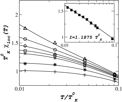
FIG. 1.: Static local susceptibility vs. $T$ for $I/T^{0}_{K}$ = 0 (+), 0.75 ($\ast$), 1 ($\times$), 1.0625 ($\Box$), 1.125 ($\Diamond$), 1.1875 (O) and 1.25 ($\triangle$). The solid lines are the fits described in the text. Inset: results for $I=1.1875\;T^{0}_{K}$, with $\delta(T=0)=5\times 10^{-3}$.

We have directly studied the physically relevant case [Eq. (12)] numerically using the QMC algorithm of Refs. [15, 24]. Starting from a trial $\chi_{0}^{-1}(\tau)$, we compute $\chi_{\text{loc}}(\tau)$. A new $\chi_{0}^{-1}(\tau)$ is then obtained from the self-consistency Eq. (LABEL:self-consistent), and the process is repeated until convergence is achieved. The results reported below are obtained for $\kappa_{c}=\pi$ [cf. Eq. (15)]. In this special case, the model can be solved exactly at $I=0$, providing a check on the QMC algorithm [15]. We choose $N_{0}\Gamma=0.19$ such that the bare Kondo scale (the inverse of the static local susceptibility at $I=0$), $N_{0}T^{0}_{K}=0.17$, is well above the lowest temperature attainable in our simulations, $T_{min}=10^{-2}\;T^{0}_{K}$. The number of Trotter time slices used varies between 64 (for the higher temperatures) and 512 (for the lowest one). We perform between $10^{4}$ and $10^{6}$ MC steps per time slice and between five and twenty self-consistency iterations. The numerical error is controlled by the last step. We estimate that the calculated susceptibilities are accurate to within 3%.

Fig. 1 shows the temperature dependence of $\chi_{\text{loc}}(\omega=0)$ for several values of $I$. The results exhibit very little $I$-dependence above $T\approx 0.1\;T^{0}_{K}$. At lower temperatures, a saturation of $\chi_{\text{loc}}$ at an $I$-dependent value is seen in the five lower curves. The two upper curves show no saturation; instead, the results are consistent with a logarithmic $T$-dependence as shown in the inset of Fig. 1, which contains data at many more points of temperature.

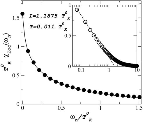
FIG. 2.: Matsubara-frequency dependence of $\chi_{\text{loc}}$ at $T=0.011\;T^{0}_{K}$ and $I=1.1875\;T^{0}_{K}$. The solid line is the fit obtained from the Hilbert transform of Eq. (26). Inset: the same data on a logarithmic plot with the point at $\omega_{n}=0$ excluded. The dashed line is the predicted critical behavior [10,11] with $\alpha=0.72$ and $\Lambda=1.54\;T^{0}_{K}$.

To interpret these numerical results, and inspired by the arguments developed earlier, we use the following fitting function for $\chi_{\text{loc}}^{\prime\prime}(\omega)$:

$$\chi_{\text{loc}}^{\prime\prime}(\omega)={\alpha\over 2I}\Theta\left(\Lambda-|\omega|\right)\;{\pi\over 2}\tanh\left({\omega\over\Lambda\;\delta}\right)\;,$$ (26)

where $\alpha$, $\Lambda$, and $\delta$ are fitting parameters that may depend on $I$ and $T$. The parameter $\delta$ is a measure of the proximity to the QCP as Eq. (26) implies that $\chi^{-1}({\bf Q})=2I\delta^{\alpha}$ for $\delta\ll 1$. By Hilbert transforming Eq. (26) we obtained an analytic expression for $\chi_{\rm loc}(i\omega_{n})$ that we used to analyze the numerical results.

In the parameter region $T<0.1\;T^{0}_{K}$, $1<I/T^{0}_{K}<1.25$ all our data can be fitted with a single value of $\alpha=0.72\pm 0.01$ and $\Lambda=1.54\;T^{0}_{K}$. The error bar represents the amplitude of variation of $\alpha$ when it is allowed to freely adjust for each value of $I$ and $T$ in the critical region. The fits are of excellent quality as shown in Fig. 2 where we display results obtained for $I=1.1875\;T^{0}_{K}$ at $T=0.011\;T^{0}_{K}$. The fitted values of $\chi_{\rm loc}(\omega_{n}=0)$ are represented by the solid lines in Fig. 1. We found in addition that, within this range of values of $I$ and $T$, the fitted $\delta(I,T)$ can be described by the phenomenological expression $\delta\propto[\delta_{0}(I)+\sqrt{\delta^{2}_{0}(I)+4(T/T^{0}_{K})^{2}}]/2$ that can be derived using Eq. (26) in the normalization condition (17). The parameter $\delta_{0}$, that decreases linearly with increasing $I$, allows us to determine the location of the QCP from the criterion $\delta(I_{c},T=0)=0$: $I_{c}\approx 1.2\;T^{0}_{K}$.

We have also computed $\chi^{-1}({\bf Q})$, the inverse of the static peak susceptibility. Fig. 3 shows that $\chi^{-1}({\bf Q})\propto\delta^{0.72}$ for $I$ and $T$ in the quantum critical regime. Our numerical value for $\alpha$ [26] is very close to that seen [5] in the Ising-like system ${\rm CeCu_{6-x}Au_{x}}$.

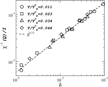
FIG. 3.: Scaling plot of $\chi^{-1}(Q)$ near the QCP.

The region $I>I_{c}$ will be discussed elsewhere[25].

We stress that a simultaneous treatment of the Kondo and RKKY couplings is crucial for our conclusion that the LCP solution is indeed self-consistent.

Some questions have recently been raised concerning the matching of the logarithmic terms in the LCP solution [11, 14] in the isotropic model. Burdin et al. [14] carried out large-$N$ and numerical analyses for zero Kondo coupling. They found that the spin liquid (SL) phase [28, 29] is unstable at low $T$ and conjectured that the LCP solutions may not be self-consistent either. Since the SL phase corresponds to the stable fixed point of the effective impurity model [27] this analysis covers a different parameter regime and is complementary to ours. By directly accessing the unstable fixed point, our results establish that the logarithmic terms are self-consistent in the Ising case. Whether numerical and analytical (beyond RG) studies in the isotropic case will yield a self-consistent LCP similar to what we have shown here for the anisotropic model is left for future work.

In summary, we have numerically identified a LCP solution in an anisotropic Kondo lattice model. The exponent for the ${\bf q}-$dependent dynamical susceptibility is fractional and is close to the experimental value.

We would like to thank S. Burdin, M. Grilli, M. J. Rozenberg (D.R.G.), K. Ingersent, S. Rabello, J. L. Smith, L. Zhu (Q.S.) and J. Zhu for discussions and collaborations on related problems, A. Georges, G. Kotliar, A. Rosch, S. Sachdev and M. Vojta for useful discussions, and NSF (Grant No. DMR-0090071), Research Corporation, Robert A. Welch Foundation, and TCSAM (Q.S.) for support. Q.S. also acknowledges the hospitality of SPhT-CEA/Saclay and Aspen Center for Physics.

REFERENCES

- [1] G. R. Stewart, Rev. Mod. Phys. 73, 797 (2001).
- [2] C. M. Varma et al., Phys. Rep. 361, 267 (2002).
- [3] P. Coleman et al., J. Phys. Cond. Matt. 13, R723 (2001).
- [4] For a review, see S. Sachdev, Quantum Phase Transitions (Cambridge Univ. Press, Cambridge, 1999), chap. 12.
- [5] A. Schröder et al., Nature 407, 351 (2000).
- [6] O. Stockert et al., Phys. Rev. Lett. 80, 5627 (1998).
- [7] P. Gegenwart et al., Acta Phys. Pol. B34, 323 (2003).
- [8] K. Ishida et al., Phys. Rev. Lett. 89, 107202(2002).
- [9] W. Montfrooij et al., cond-mat/0207467.
- [10] Q. Si et al., Nature 413, 804 (2001).
- [11] Q. Si et al., Phys. Rev. B, in press (cond-mat/0202414).
- [12] P. Coleman et al., Phys. Rev. B 62, 3852 (2000).
- [13] S. Sachdev and T. Morinari, Phys. Rev. B 66, 235117 (2003).
- [14] S. Burdin, M. Grilli, and D. R. Grempel, Phys. Rev. B 67, 121104 (2003).
- [15] D. R. Grempel and M. J. Rozenberg, Phys. Rev. B 60, 4702 (1999).
- [16] A. M. Sengupta and A. Georges, Phys. Rev. B 52, 10295 (1995).
- [17] S. Sachdev et al., Phys. Rev. B 52, 10286 (1995); J. Ye et al., Phys. Rev. Lett. 70, 4011 (1993).
- [18] Q. Si and J. L. Smith, Phys. Rev. Lett. 77, 3391 (1996).
- [19] J. L. Smith and Q. Si, Phys. Rev. B 61, 5184 (2000).
- [20] R. Chitra and G. Kotliar, Phys. Rev. Lett. 84, 3678 (2000).
- [21] H. Kajueter, Rutgers University Ph. D. thesis (1996).
- [22] G. Kotliar and Q. Si, Phys. Rev. B53, 12373 (1996).
- [23] The fractional arises as follows. The critical local susceptibility of the impurity problem [Eqs. (12,8), with ] is . The amplitude in general depends on and in a non-trivial way. The self-consistency condition [which follows from Eq. (20)] specifies and, through Eq. (22), also . In the limit of Eq. (14), however, is “pinned” to . Even though the destruction of the Kondo effect still takes place, is no longer determined by the leading terms of and alone; considerations of the subleading terms yield an that is not fractional. Recent work [S. Pankov et al., cond-mat/0304415] shows that such a pinning of the critical amplitude persists to order .
- [24] D. R. Grempel and M. J. Rozenberg, Phys. Rev. Lett. 80, 389 (1998); M. J. Rozenberg and D. R. Grempel, ibid. 81, 2550 (1998).
- [25] J. Zhu, D. Grempel, and Q. Si, cond-mat/0304033
- [26] We have also studied three other parameter sets for which = 0.03, 0.085, and 0.25. The exponent turns out to be essentially the same suggesting that, for the Ising-like model, is nearly universal.
- [27] L. Zhu and Q. Si, Phys. Rev. B 66, 024426 (2002); G. Zaránd and E. Demler, ibid., 024427 (2002).
- [28] S. Sachdev and J. Ye, Phys. Rev. Lett. 70, 3339 (1993).
- [29] O. Parcollet and A. Georges, Phys. Rev. B 59, 5341 (1999).