Optical Properties of Layered Superconductors near the Josephson Plasma Resonance

Abstract

We study the optical properties of crystals with spatial dispersion and show that the usual Fresnel approach becomes invalid near frequencies where the group velocity of the wave packets inside the crystal vanishes. Near these special frequencies the reflectivity depends on the atomic structure of the crystal provided that disorder and dissipation are very low. This is demonstrated explicitly by a detailed study of layered superconductors with identical or two different alternating junctions in the frequency range near the Josephson plasma resonance. Accounting for both inductive and charge coupling of the intrinsic junctions, we show that multiple modes are excited inside the crystal by the incident light, determine their relative amplitude by the microscopic calculation of the additional boundary conditions and finally obtain the reflectivity. Spatial dispersion also provides a novel method to stop light pulses, which has possible applications for quantum information processing and the artificial creation of event horizons in a solid.

]

I Introduction

The problem of optical properties of crystals with spatial dispersion has remained challenging since the original paper of Pekar on the optics of exciton bands [1]. Despite considerable effort, the complete theoretical description of the optical properties of such systems is still missing [2, 3, 4, 5, 6, 7, 8].

The nontrivial optical features of crystals with a dispersive dielectric function $\epsilon(\omega,{\bf k})$ are based on the fact that incident light with a given frequency excites several eigenmodes with different wave vectors ${\bf k}$. This poses the fundamental problem that the Maxwell boundary conditions, i.e. the continuity of the electric and magnetic field components parallel to the surface, are insufficient to calculate the relative amplitudes of these modes and consequently to describe physical quantities, such as reflectivity or transmissivity. Since the early work of Pekar [1, 2] and Ginzburg [3] this difficulty was usually addressed in a purely phenomenological approach by introducing so called additional boundary conditions (ABC) for the macroscopic polarization. These ABC are motivated physically by the microscopic structure of the surface, but the choice of ABC is not universal and may be controversial, see Ref. [4] and Comments to this paper. Only the complete solution of the microscopic model can determine the dependence of the reflectivity on the microstructure unambiguously.

Such a solution was found recently for the first time for the reflectivity near the Josephson plasma resonance (JPR) in highly anisotropic layered superconductors [9], which is an interlayer charge oscillation due to the tunneling of Cooper pairs and quasiparticles in highly anisotropic layered superconductors [10, 11, 12]. Josephson plasma oscillations inside layered superconductor may be excited by the light incident to the surface of the crystal in the geometries (a) or (b) shown in Fig. 1. The JPR in layered superconductors is the simplest example, which illuminates the effects of spatial dispersion and the discrete atomic structure on optical properties in strongly anisotropic materials. Here we will describe the method of the calculations in [9] in more detail, generalize our results for the JPR to different geometries, discuss the various transmission and reflection coefficients in a finite size sample and point out perspectives to stop light with the help of spatial dispersion. We also stress that the discrete atomic structure within the unit cell can have similar effects as spatial dispersion.

FIG. 1.: The geometry of the layered system showing the incident and reflected light at the surface of incidence (a) parallel and (b) perpendicular to the layers. Interlayer charge oscillations (vertical arrows) are excited by the component of the electric field perpendicular to the layers.

In the framework of the Lawrence-Doniach model [13] (interlayer Josephson coupling) we can describe both layered superconductors with identical intrinsic Josephson junctions (such as Tl-2201 [14, 15], Bi₂Sr₂CaCu₂O₈ [16], the organic material $\kappa$-(BEDT-TTF)₂-Cu(NCS)₂ [17, 18] or (LaSe)(NbSe${}_{2})$ [19, 20]) and compounds, where different junctions alternate like in SmLa_1-xSr_xCuO_4-δ [21, 22, 23, 24, 25, 26], Bi-2212/Bi-2201 [27] or atomic scale YBCO/PrBCO superlattices [28]. Thereby we take into account not only the dispersion of the plasma mode caused by the inductive interaction of currents parallel to the layers, but also the $c$-axis dispersion due to charge fluctuations on the layers [29, 30, 31, 32, 33, 34].

The JPR is an ideal choice to illustrate the effect of spatial dispersion and the atomic structure on optical properties both theoretically and experimentally. First of all, recent optical experiments on the layered superconductor SmLa_1-xSr_xCuO_4-δ with T^∗ crystal structure showed evidence that the spatial dispersion of the Josephson plasmon in the direction perpendicular to the layers is important [21, 22, 23, 24, 25]. For incidence parallel to the layers, see Fig. 1(b) at $\theta=0$, two peaks at $\approx 7$ and $\approx 12$ cm^-1 were observed in reflection, which can be naturally understood as the JPR [21] of alternating intrinsic junctions with SmO or LaO in the barriers between the CuO₂-layers [21, 22, 23, 24, 25, 35]. The very high ratio of the peak intensities, about 20, cannot be explained in a dispersionless model [36] and it points to a quite strong $c$-axis dispersion of the plasma modes due to charge variations [37, 38]. Secondly, from the theoretical point of view the well established Lawrence-Doniach model [13] formulated in terms of finite-difference equations for electromagnetic fields and phases of the superconducting order parameter is sufficient to provide a complete microscopic description and can be solved analytically. Lastly, it is fortunate that the damping due to dissipation is low, because at low temperatures the JPR frequency is well below the superconducting gap and the quasiparticles responsible for dissipation are frozen out. Otherwise it would strongly overshadow the effects of dispersion or the atomic structure as described below.

Extracting the strength of the $c$-axis dispersion in high temperature superconductors is important in its own, as the dynamics of Josephson oscillations in layered superconductors is strongly influenced by it [30, 32, 33]. It is also intimately connected with the electronic compressibility of the superconducting CuO₂-layers, which is hard to measure in situ otherwise and contains unique information about the electronic many-body interactions in the layers.

From a more fundamental point of view, we show that in the presence of spatial dispersion the conventional Fresnel formulas for reflectivity and transmission have to be modified substantially near certain frequencies, if both the dissipation and the crystal disorder are weak. Usually it is assumed that the optical properties of crystals are completely determined by average, bulk properties described by a frequency dependent dielectric function $\epsilon(\omega)$, but not by the explicit spatial dispersion (${\bf k}$-dependence) or the specific atomic structure of the crystal (implicit spatial dispersion). This is based on the notion that the wave length of light is much larger than the atomic length scales and therefore light is expected to be influenced only by averaged properties of the crystal. Here we will stress out that this approach breaks down, if the group velocity, ${\bf v}_{g}=\partial\omega({\bf k})/\partial{\bf k}$, of the wave packet of the optical excitation with dispersion $\omega({\bf k})$ becomes small. The physical reason for this breakdown of the macroscopic theory is the appearance of a small effective wave length, $\lambda_{g}=v_{g}/\omega$, related to the slow motion of the wave packet, which can be comparable with the interatomic distance.

The conditions, when the group velocity becomes small, can be most easily seen for an isotropic medium described by the dielectric function $\epsilon(\omega,k)$. Then the dispersion relation of an optically excited eigenmode is $c^{2}k^{2}=\omega^{2}\epsilon(\omega,k)=\omega^{2}n^{2}(\omega,k)$. For a transversal wave the implicit derivative of this equation with respect to $k$ leads to

$$v_{g}=\frac{d\omega}{dk}=\frac{c-\frac{\omega}{2\sqrt{\epsilon}}~{}\frac{\partial\epsilon}{\partial k}}{\sqrt{\epsilon}+\frac{\omega}{2\sqrt{\epsilon}}~{}\frac{\partial\epsilon}{\partial\omega}}=\frac{\omega}{k}\frac{1-k\frac{\partial\ln n}{\partial k}}{1+\omega\frac{\partial\ln n}{\partial\omega}}.$$ (1)

From Eq. (1) it is clear that light can be slowed down (a) due to a strong frequency dispersion $\omega dn(\omega)/d\omega\gg 1$ (as discussed in [39, 40]), (b) due to a small value $1-k\partial\ln n/\partial k$, i.e. when the spatial dispersion is strong or, (c) when the wavevector $k$ becomes large. In the absence of spatial dispersion in the dielectric function the conditions (a) and (c) are fulfilled at frequencies corresponding to a pole in $\epsilon(\omega)$, where both $dn/d\omega$ and the wavevector $k$ are large, cf. $k^{2}\propto\epsilon(\omega)$. Furthermore, it is expected that in the same frequency region the dielectric function is also quite sensitive to the wave vector, i.e. explicit spatial dispersion is significant, cf. case (b).

Accounting for the wavevector dependence of the dielectric function, in general leads to multiple solutions of the dispersion relation $c^{2}k^{2}=\omega^{2}\epsilon(\omega,k)$ for the wave vectors $k_{zp}$, $p=1,2$, along the direction $z$ perpendicular to the surface at given $\omega$ in the geometry shown in Fig. 1(a). As it will be derived below, only the light-like modes with small $|k_{zp}|$ contribute significantly to the transmission and the usual one mode Fresnel result is recovered, if $|k_{z1}|\ll|k_{z2}|$. On the other hand, the conventional description breaks down, when both $|k_{zp}|$ are comparable and contribute to the optical properties. This happens if a pole in the dispersionless theory, which corresponds to the cases (a) and (c) of low group velocity, is regularized by the introduction of spatial dispersion.

Depending on the type of the spatial dispersion the excited modes may be both real (propagating modes) or one wave vector may be real, while the other one is complex (decaying mode). This leads to two types of critical frequencies, where the Fresnel approach becomes invalid. Namely it occurs at frequencies $\omega_{e}$, where both $k_{z}$ are real and $|k_{z1}|\approx|k_{z2}|$, and at frequencies $\omega_{i}$, where $k_{z1}\approx ik_{z2}$.

FIG. 2.: Schematic mixing of a transverse optical phonon characterized by anomalous dispersion with a propagating electromagnetic wave leads to an extremal point $\omega_{e}$ in the lower polariton band, where the group velocity vanishes. Just below the frequency $\omega_{e}$ two modes with similar wavevectors propagate.

When both modes are propagating, $v_{g}$ vanishes at frequencies $\omega_{e}$ due to strong spatial dispersion, the case (b) mentioned after Eq. (1), see Fig. 2. In general, this case occurs, if the eigenmodes of the crystal, when decoupled from electromagnetic waves, have a dispersion opposite to that of the electromagnetic wave. Generic examples are phonon modes with anomalous (decreasing) dispersion mixing with propagating light of normal dispersion, which form a polariton (cf. Fig. 2), or the Josephson plasmon with normal dispersion interacting with screened electromagnetic waves in a superconductor, which show an anomalous dispersion, see Sects. III.B and IV below. As the main consequence, near frequencies $\omega_{e}$ the transmission coefficient into the crystal is not determined solely by the dielectric function, but crucially depends on the microstructure of the crystal near the surface, if both dissipation and disorder are very low and the system is strongly anisotropic. We will also show that interfering multiple propagating waves create a behavior similar to intrinsic birefringence and affect strongly the transmission through the crystal and multiple reflection.

In the second situation (one mode is propagating, while another is decaying) the Fresnel approach breaks down near frequencies $\omega_{i}$, where the moduli of the wave vectors of two excited modes become equal. Near these frequencies both $|k_{zp}|$ become large, of the order of the inverse interatomic spacing, which leads to a small, but finite group velocity $v_{g}$ as described in the case (c) after Eq. (1). This occurs, for example, for Josephson plasmons with anomalous dispersion in a crystal with different alternating junctions, where one plasmon has normal, while the other one has anomalous dispersion, see Sect. IV below. As near the frequencies $\omega_{i}$ only a single mode propagates into the crystal, the transmission coefficient is significantly suppressed in comparison with resonances at extremal points $\omega_{e}$, where incident light excites two propagating modes.

FIG. 3.: A pole in $k_{z}^{2}(\omega)$ in the case without spatial dispersion (dashed line) indicates the importance of small length scales due to the low group velocity (cf. Eq. (1)) and the breakdown of the macroscopic theory based on a $k_{z}$-independent dielectric tensor. For an isotropic system this corresponds to a singularity in the dielectric function, $k_{z}^{2}\propto\epsilon(\omega)$ This pole is regularized, when spatial dispersion is taken into account, and depending on the sign of $dk_{z}^{2}/d\omega$ an extremal point $\omega_{e}$, where the group velocity vanishes, appears as shown in a), or as shown in b), the singularity transforms into a special frequency $\omega_{i}$, where $k_{z1}^{2}=-k_{z2}^{2}$.

In Fig. 3 it is demonstrated schematically, how the critical frequencies $\omega_{e}$ and $\omega_{i}$, where the amplitudes of the exited multiple modes equal, $|k_{z1}|=|k_{z2}|$, develop from a singularity in the one mode theory, which neglects the $k_{z}$-dependence of the eigenmodes. In the simplest case of an isotropic medium, which was considered after Eq. (1), the dispersionless dielectric function and squared wavevector amplitudes are proportional, $\epsilon(\omega)\propto k^{2}$, and their poles coincide. The breakdown of the one mode Fresnel theory at these points is already anticipated from the low group velocity $v_{g}$, due to the large frequency dispersion, $|dk_{z}/d\omega|\gg 1$, and the large $|k_{zp}|$ near the pole, cf. case (a) and (c) in the discussion after Eq. (1).

If for the crystal dispersion (without coupling to electromagnetic waves) $dk_{z}^{2}/d\omega<0$, an extremal point $\omega_{e}$ appears below the singularity and at this frequency $\omega_{e}$ the group velocity $v_{gz}=d\omega/dk_{z}$ vanishes and two propagating modes with $k_{z1}=-k_{z2}$ are excited, see Fig. 3 (a). In a similar way, at the extremum of $\omega(k_{z}^{2})$ above the singularity the imaginary excited modes merge, $k_{z1}^{2}=k_{z2}^{2}<0$, while in the intermediate frequency region the solutions $k_{zp}^{2}$ are complex. On the other hand, if $dk_{z}^{2}/d\omega>0$, the singularity in the dispersionless one mode theory is transformed to a special point $\omega_{i}$, where the amplitude of the excitation equals, but one is propgating and the other decaying, $k_{z1}^{2}=-k_{z2}^{2}$.

Remarkably, a special point $\omega_{i}$ can appear, when the group velocity is small, even without a wavevector dependence (i.e. without explicit spatial dispersion) in the dielectric function due to the atomic structure in the unit cell alone (implicit spatial dispersion). Generally for each polariton band a real or imaginary mode is excited, but usually inside one band the second wave associated with the off-resonant excitation of the other bands can be neglected. Here it will be shown that this assumption breaks down, when the group velocity becomes small, e.g. for large amplitudes of the wavevectors, cf. case (c). Thereby the system with alternating plasma resonances like SmLa_1-xSr_xCuO_4-δ with light incident parallel to the layers (Fig. 1(b) at $\theta=0$) presents a generic example, as in this case the wavevector $k_{z}$ perpendicular to the layers (explicit spatial dispersion) vanishes due to the homogeneity of the incident beam. In a macroscopic theory the electrodynamic response to the electric field, which is averaged within the unit cell, is decribed by the effective (average) dielectric function ${\tilde{\epsilon}}_{c}(\omega)$,

$$\frac{1}{\tilde{\epsilon}_{c}(\omega)}=\frac{1}{2}\left[\frac{1}{\epsilon_{c1}(\omega)}+\frac{1}{\epsilon_{c2}(\omega)}\right].$$ (2)

Thereby a pole in ${\tilde{\epsilon}_{c}(\omega)}$ appears between the zeros of $\epsilon_{cl}(\omega)=\epsilon_{c0}(1-\omega_{c0,l}^{2}/\omega^{2})$ ($l=1,2$, $\epsilon_{c0}$ background dielectric constant), which correspond to the plasma frequencies $\omega_{c0,l}$ in the different junctions [36, 37]. This indicates the breakdown of the one-mode Fresnel approach and the necessity to account properly for the second solution. Obviously, similar consequenses of such a ”discrete” implicit spatial dispersion are expected generally for any crystals with multiple optically active crystal bands of the same symmetry.

Both the behavior near $\omega_{e}$ and $\omega_{i}$ are in contrast to the conventional Fresnel theory and to the common believe that spatial dispersion of crystal modes or the atomic structure do not create measurable effects of order unity in optical properties, but only enter in negligible corrections proportional to the ratio of atomic scales and the wavelength of light. In fact, the Fresnel results have to be modified significantly in a narrow interval near the frequencies $\omega_{e}$ and $\omega_{i}$, but only in perfect crystals with very weak dissipation.

Finally, we point out that the vanishing of the group velocity at extremal frequencies $\omega_{e}$ due to spatial dispersion of the crystal modes provides a novel way to stop light pulses dynamically. Recently it attracted a considerable interest to diminish the light velocity strongly with the help of frequency dispersive gaseous media as described by case (a) after Eq. (1). From a practical point of view, our suggestion based on the ${\bf k}$-dependence of the dielectric tensor allows to use slow light in a solid state device for the processing of information. In particular, the sensitivity of the group velocity in solids to the external fields could be used to store quantum information in the form of photonic qubits, as required for optical quantum computers [41]. Our novel solid state proposal to stop light might be of advantage compared with the realizations using gaseous media, as it is easier to scale to larger system sizes and more complex devices. By adjusting an inhomogeneous external parameter, like the magnetic field for the JPR, a spatially inhomogeneous profile for the group velocity can be imprinted. Such conditions can simulate in the laboratory the behavior of light in a curved spacetime, as realized in astrophysical situations, e.g. near the event horizon of a black hole [42].

Previously the spatial dispersion of the Josephson plasma mode and its effect on the propagating electromagnetic waves in layered superconductors with identical Josephson junctions was discussed by Tachiki, Koyama and Takahashi [31]. They realized that the mixing of plasma modes with electromagnetic waves can lead to two propagating waves with different wave vectors for the same frequency. However, implications of this fact to the optical properties, like reflectivity, were not discussed. Van der Marel and Tsvetkov [37] present an effective dielectric function for the system with alternating Josephson junctions and charge coupling within the unit cell for the special case of incidence parallel to the layers, but they did not account correctly for the dissipation due to the conductivities and for the nontrivial effects of the “discrete” spatial dispersion mentioned above.

The paper is organized as follows: In the first part, we derive in general the optical properties of an uniaxial crystal with explicit spatial dispersion along the symmetry axis in the dielectric function using additional boundary conditions with one phenomenological parameter (Sect. II). In the second part, we confirm these results for oblique incidence in the microscopic model for the JPR accounting for the atomic (layered) structure. Thereby the ABC are derived and analytical solutions for systems with identical (Sect. III) and two different alternating (Sect. IV) Josephson junctions are obtained. In Sect. V the atomic structure is taken into account to derive the reflectivity in the incidence parallel to the layers. Technical details are given in the Appendices.

II Macroscopic approach for crystals with spatial dispersion

In this Section we derive the dispersion relation from a macroscopic dielectric tensor (Sect. II.A), calculate the transmission coefficients into (II.B) and through (II.C) the crystal using a phenomenological ABC and close with some further remarks, concerning e.g. future applications, like the stopping of light (II.D).

A Dispersion relation

We consider the geometry of the incident and reflected light as shown in Fig. 1. The wave vector of the incident light with frequency $\omega$ for the geometry shown in Fig. 1(a) is ${\bf k}_{0}=(\omega\sin\theta/c,0,\omega\cos\theta/c)$, while for Fig. 1(b) ${\bf k}_{0}=(\omega\cos\theta/c,0,\omega\sin\theta/c)$, where the $z$-axis is perpendicular to the layers (it coincides with the $c$-axis of the crystal). The incident (quasi-monochromatic) electromagnetic wave is assumed to be P-polarized, i.e. the electric field ${\bf E}({\bf r},t)={\bf E}(\omega,{\bf k})\exp(i{\bf k}{\bf r}-i\omega t)$ is in the plane defined by ${\bf k}_{0}$ and the normal of the surface ($xz$-plane), while the magnetic field ${\bf B}$ has only a component in $y$-direction. S-polarization is not considered here, as an electric field parallel to the layers does not excite the JPR studied below.

In the macroscopic approach used here we describe the crystal by a dielectric tensor, which is averaged on atomic scales within the unit cell, but can depend on the wave vector (explicit spatial dispersion), and study the effects of the intrinsic microstructure (implicit spatial dispersion) in Sect. V.

In the following we will consider highly anisotropic uniaxial (layered) crystals with the dielectric function components $\epsilon_{c}(\omega,k_{z})$ along the $c$-axis ($z$-axis) and $\epsilon_{a}(\omega)$ in the $ab$ ($xy$) plane along the layers in a parameter regime appropriate for the JPR. In $\epsilon_{c}(\omega,k_{z})$ we account for a collective mode (JPR in our case), which is strictly longitudinal with the dispersion $\omega_{c}(k_{z})$ for $k_{x}=0$, i.e. $\epsilon_{c}[\omega=\omega_{c}(k_{x}=0,k_{z}),k_{z}]=0$, and whose polarization is mainly in the $c$-direction for any $k_{x}$ due to the strong anisotropy, $|\epsilon_{a}|\gg|\epsilon_{c}|$, near the JPR. We neglect the eigenmode, which is polarized parallel to the layers for $k_{x}=0$, as it is of much higher frequency than the JPR.

From the bulk Maxwell equations for the Fourier components,

$$ck_{x}B_{y}=-\omega\epsilon_{c}(\omega,k_{z})E_{z},$$ (3)

$$k_{x}E_{z}-k_{z}E_{x}=-(\omega/c)B_{y},$$ (4)

$$ck_{z}B_{y}=\omega\epsilon_{a}(\omega)E_{x}$$ (5)

follows directly the dispersion relation,

$$\frac{k_{x}^{2}}{\epsilon_{c}(\omega,k_{z})}+\frac{k_{z}^{2}}{\epsilon_{a}(\omega)}=\frac{\omega^{2}}{c^{2}},$$ (6)

of the eigenmodes in the crystal.

For the geometry shown in Fig. 1(b) and neglecting the discrete layered structure in $z$-direction, we obtain analogously $k_{z}={\bf k}_{0z}=\omega\sin\theta/c$ of the excited crystal mode, while the dispersion relation, Eq. (6), gives a single solution for $k_{x}^{2}$. Hence, the usual Fresnel description is generally valid, except where $|k_{x}|$ becomes large, e.g. at the poles of $\epsilon_{c}(\omega)$, see Eq. (6). At these points the implicit spatial dispersion due to the atomic structure in the unit cell in multiband systems has to be taken into account. Then multiple solutions $k_{x}^{2}$ of the dispersion relation contribute, which will be discussed for the JPR with alternating junctions in Sect. V below.

In the geometry shown in Fig. 1(a) we obtain from the translational invariance parallel to the surface the wave vector component $k_{x}={\bf k}_{0x}=\omega\sin\theta/c$, and the dispersion relation determines the solution(s) for the $z$-component $k_{z}(\omega,\theta)$ of the modes excited by the incident wave.

In a crystal described by the dielectric functions $\epsilon_{a,c}(\omega)$, which is independent of the wave vector ${\bf k}$, the dispersion relation Eq. (6) has a unique solution $k_{z}^{2}(\omega)$. The Maxwell boundary conditions (MBC), requiring the continuity of the parallel components $E_{x}(z)$ and $H_{y}(z)$ at the surface $z=0$, immediately give the Fresnel formula for the reflection coefficient $R=|r|^{2}$ and the transmissivity $T=1-R$ into the crystal. Here

$$r=\frac{1-\kappa}{1+\kappa},\ \ \kappa=\frac{E_{x}(z=0)}{B_{y}(z=0)\cos\theta}.$$ (7)

When in a highly anisotropic crystal the eigenmode with electric field approximately parallel to the layers is neglected, the effective dielectric function $\epsilon_{\rm eff}$ is given by

$$\kappa=\sqrt{\epsilon_{\rm eff}}=\frac{n_{0}}{\epsilon_{a}(\omega)\cos\theta},$$ (8)

where the refraction index is

$$n_{0}=ck_{z}(\omega)/\omega=\sqrt{\epsilon_{a}(\omega)(1-\sin^{2}\theta/\epsilon_{c}(\omega))}.$$ (9)

This suggests that for an anisotropic crystal in this geometry the critical frequencies, where the refraction index $n_{0}$ becomes large and the Fresnel theory breaks down, appear at zeros of $\epsilon_{c}(\omega)$ rather than at poles of the dielectric function, as for isotropic system discussed in the introduction (cf. Eq. (1)) and Fig. 1(b).

If the dielectric function, $\epsilon_{c}(\omega,k_{z})$, is dispersive in the $c$-direction, Eq. (6) has multiple solutions for $k_{z}^{2}(\omega)$ [3, 31]. In the following we restrict ourselves to the simplest case of four (in general complex) solutions $\pm n_{1},\pm n_{2}$ for the refraction indices.

Generally, in a crystal of finite thickness, where the (multiple) back reflection from the second surface is taken into account, all four solutions $\pm n_{1,2}$ have to be considered. For simplicity, we will consider in the following mainly a semi-infinite crystal in the half space $z>0$, where only two of the solutions are physical. When dissipation is low, for quasi-monochromatic wave packets the direction of the energy transfer is determined by the Poynting vector ${\bf S}$, which is oriented along the group velocity ${\bf v}_{g}=\partial\omega/\partial{\bf k}$ [3]:

$${\bf S}=W{\bf v}_{g},$$ (10)

$$W=\frac{1}{16\pi}\left[\frac{\partial(\omega\epsilon_{a})}{\partial\omega}E_{x}^{\phantom{*}}E_{x}^{*}+\frac{\partial(\omega\epsilon_{c})}{\partial\omega}E^{\phantom{*}}_{z}E_{z}^{*}+B^{\phantom{*}}_{y}B_{y}^{*}\right].$$ (11)

Here $W$ is the high frequency average of the energy density. In agreement with the causality principle the group velocity of propagating modes in the $c$-direction, $v_{gz}=\partial\omega(k_{z})/\partial k_{z}$, should therefore be positive. Note that in the case of normal (anomalous) dispersion this requires the real part of the wave vector $k_{zp}$ (modes $p=1,2$) and of the refraction index $n_{p}=ck_{zp}/\omega$ to be positive (negative). When dissipation is taken into account, this rule is equivalent to the condition that the eigenmodes should decay inside the crystal, i.e. ${\rm Im}(k_{zp})>0$.

This has in particular consequences at extremal frequencies $\omega_{e}$ of the dispersion relation ${\rm Re}(\omega(k_{z}))$, where the group velocity $v_{gz}=0$ vanishes and two branches, one with normal and another one with anomalous dispersion merge, see Fig. 2. At these points the two solutions for $k_{z}$, which are real in the absence of dissipation, have the same amplitude $|k_{z}|$, but different signs,

$${\rm Re}[n_{1}(\omega_{e})+n_{2}(\omega_{e})]=0.$$ (12)

B Transmissivity $T$ on surface

In the macroscopic approach the electric field $E_{z}$ and the polarization $P_{z}$ in a semi-infinite crystal with a single atom in the unit cell and with the background dielectric constant $\epsilon_{c0}$ can be expressed as

$$E_{z}(z)=\sum_{p=1,2}E_{z}(k_{zp})\exp(ik_{zp}z),$$ (13)

$$P_{z}(z)=\sum_{p=1,2}E_{z}(k_{zp})\chi_{c}(k_{zp})\exp(ik_{zp}z),$$ (14)

$$4\pi\chi_{c}(k_{z})=\epsilon_{c}(\omega,k_{z})-\epsilon_{c0},$$ (15)

while the equations for $E_{x}$ and $B_{y}$, which enter in Eq. (7), are similar. In order to determine the amplitudes $E_{z}(k_{zp})$ of the different eigenmodes we use the most general ABC proposed by Ginzburg [3]

$$P_{z}(z)+\ell(\partial P_{z}/\partial z)=0,\ \ \ z\rightarrow 0,$$ (16)

where the length scale $\ell$ is a phenomenological parameter to be determined from the microscopic model. In systems with inversion symmetry we can use $\chi_{c}(\omega,k_{z})-\chi_{c}(\omega,0)\sim k_{z}^{2}$ for $k_{z}\rightarrow 0$ and obtain

$$\sum_{p}E_{z}(k_{zp})(1+i\xi n_{p})=0,\ \ \ \xi=\omega\ell/c.$$ (17)

in leading order in $\epsilon_{a}/n_{p}^{2}\ll 1$ and $1/|n_{1}n_{2}|\ll 1$. In this limit Eq. (17) and the following results are confirmed microscopically for the JPR in Sect. III and IV, while in general corrections involving field components parallel to the surface have to be considered in Eq. (16). Using Eqs. (5), (6) and (17), we derive (near the resonance)

$$\kappa=\frac{1}{\epsilon_{a}\cos\theta}~{}\frac{n_{1}n_{2}}{n_{1}+n_{2}-i\xi n_{1}n_{2}}.$$ (18)

We see that in the case of multiple eigenmodes in the crystal the optical properties like the reflectivity generally cannot be expressed by the refraction indices $n_{p}$ alone, which are determined by the bulk dielectric functions $\epsilon_{a,c}$ via Eq. (6), but also depend explicitly on the parameter $\xi$ introduced by the boundary conditions.

As the wavelength $\lambda$ of light is larger than all length scales related to the atomic structure of the crystal or to the change of the polarization at the surface, we can assume $\xi\sim\ell/\lambda\ll 1$. Therefore the term $\xi n_{1}n_{2}$ can be neglected everywhere except at the extremal frequencies $\omega_{e}$, where ${\rm Re}(n_{1}+n_{2})=0$.

If in addition the amplitude of one excited mode is large, i.e. $|n_{2}|\gg|n_{1}|$ and $|n_{1}n_{2}|\gg|\epsilon_{a}|$, the conventional one mode Fresnel result, Eq. (8), is obtained for the mode with smallest $n$. In Fig. 2 it can be seen that for the phonon polariton away from the extremal frequency $\omega_{e}$ this condition is fulfilled and only the usual light-like mode remains.

Deviations from the usual Fresnel theory are therefore expected, when the amplitudes of $n_{1}$ and $n_{2}$ are comparable and both modes play a role. The resonances in the transmissivity are located in these two mode frequency regions and we distinguish the cases that (i) both excited modes are propagating ($n_{1,2}$ real) or (ii) one mode is propagating, while the second is decaying ($n_{1}$ real, $n_{2}$ imaginary). The appearance such type of special frequencies $\omega_{e}$, where $n_{1}=-n_{2}$, and $\omega_{i}$, where $n_{1}=in_{2}$, near a pole in the refraction index of the dispersionless one mode theory is schematically shown in Fig. 3 (the index of $\omega_{i}$ reminds of the factor $\pm i$ between the solutions $n_{1,2}$).

(i) For two real modes $n_{1,2}$ we have ${\rm Re}(n_{1}+n_{2})=0$ at the extremal point $\omega=\omega_{e}$, when causality is taken into account, see Eq. (12). Then, if the dissipation is weak in addition, e.g. ${\rm Im}(n_{1}+n_{2})\ll|\xi n_{1}n_{2}|$, only the term $i\xi n_{1}n_{2}$ in Eq. (18) remains, $\kappa(\omega_{e})$ is imaginary and $T(\omega_{e})=0$. The transmissivity $T$ reaches its maximum at the frequency $\omega_{{\rm e,max}}$ slightly above $\omega_{e}$. At this frequency

$$(n_{1}+n_{2})=\epsilon_{a}^{-1}n_{1}n_{2}(\cos^{-2}\theta+\xi^{2}\epsilon_{a}^{2})^{1/2},$$ (19)

$$T_{\rm e,max}=2/[(1+\xi^{2}\epsilon_{a}^{2}\cos^{2}\theta)^{1/2}+1].$$ (20)

It is pointed out that both the position $\omega_{\rm e,max}$ of the resonance in $R$ or $T$ and its amplitude are determined not solely by the imaginary part of $\epsilon_{a,c}$ as in the dispersionless case, but also by the surface parameter $\xi$. This correction is important for highly anisotropic systems, where $\xi\epsilon_{a}\gg 1$, although $\xi\ll 1$, as it is realized for the JPR (see Eq. (74)). We see that in the absence of dissipation $T_{\rm e,max}$ depends on $\xi$ and is generally smaller than the Fresnel result $T_{\rm max}=1$, see Fig. 5. Physically this result reflects the fact that the low group velocity near $\omega_{e}$ introduces a small length scale $\lambda_{g}=v_{g}/\omega$, which makes the variation of the polarization $P_{z}$ near the surface relevant and indicates the breakdown of the translational invariance on the atomic scale $l$. Note that the opposite signs of the refraction indices $n_{1,2}$ near $\omega_{e}$ due to causality are essential for the dependence of $T_{\rm e,max}$ on $\xi$. The vanishing of $n_{1}+n_{2}$ at $\omega_{e}$ (see Eq. (12)) in Eq. (18) and its consequences in Eqs. (19) and (20) have not been noted previously [1, 2, 3, 4, 7, 8]. We also note that the results in Eqs. (19) and (20) cannot be obtained from the ABC proposed by Pekar [1, 2], which neglects the derivative in Eq. (16).

(ii) In the case, when $n_{1}$ is real, while $n_{2}$ is imaginary without dissipation, we anticipate that $T$ is strongly suppressed, because both modes are excited by the incident light, but only a single mode propagates into the crystal. This situation occurs e.g. in superconductors when the dispersion of the collective mode is anomalous (cf. Fig. 11 in Section IV). $T(\omega)$ is in this case peaked at critical frequencies $\omega_{i}$ near $\omega_{c}$, where $n_{2}=-in_{1}$ with $n_{1}<0$. Here we obtain for the maximal transmission coefficient

$$T_{{\rm i,max}}=T(\omega_{i})=\frac{2n_{1}}{\epsilon_{a}\cos\theta},$$ (21)

so that $T(\omega_{i})\ll T_{{\rm e,max}}$. This difference in the resonance amplitude, depending whether two or one propagating modes are excited, cannot be described in the one mode Fresnel approach without spatial dispersion, where in both cases a single propagating mode is excited and the transmission amplitudes are comparable. This observation and the strong deviation from the conventional Fresnel result is confirmed below for the JPR in Sect. IV. In contrast to the situation (i) near extremal points $\omega_{e}$, the parameter $\xi$ is irrelevant near $\omega_{i}$.

C Transmission through thin film

FIG. 4.: Transmission amplitudes of the wave with refraction index $n_{p}$ into ($t_{p}$) and out of ($\tau_{p}$) the crystal and multiple reflections at the first ($R_{n}$) and the second surface ($\rho_{pp^{\prime}}$).

We now study the transmission and back reflection of the multiple excited modes in a thin film of finite thickness $L$, see Fig. 4. For the ratio of the magnetic field $t_{p}B_{y}^{\rm in}$ of a partial wave with the refraction index $n_{p}$ ($p=1,2$) excited in the crystal to that of the incident wave $B_{y}^{\rm in}$ we obtain

$$t_{p}=i(-1)^{p}\frac{2(1-i\xi n_{p})}{\xi(n_{2}-n_{1})(1+\kappa)}.$$ (22)

We will see that $|t_{p}|>1$ for JPR, e.g. the fields of the two partial waves are enhanced, but have opposite direction. Note that the transmissivity $T$ follows from the ratios of the $z$-components of the Poynting vectors, Eq. (10), and that $T\neq|t_{1}+t_{2}|^{2}$.

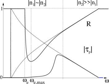
FIG. 5.: Reflectivity $R=1-T$ and ratio $|\tau_{p}|$ of the outgoing magnetic fields at the second surface of the crystal near an extremal point $\omega_{e}$ with (solid line) and without (dashed) spatial dispersion without dissipation (schematically). Compared with the conventional Fresnel formulas the plasma edge in $R$ is at the higher frequency $\omega_{e}$ and the amplitude of the resonance at $\omega_{\rm e,max}$ is damped due to $\xi$ in Eq. (18). The amplitude $\sim|\tau_{p}(\omega_{\rm e,max})|$ of the outgoing waves (cf. Eq. (24)) is strongly suppressed in the frequency region, where R is minimal, e.g. where the transmission $T$ into the crystal is maximal (Eq. (27)).

At the second surface of a crystal the arriving wave with index $n_{p}$ ($p=1,2$) and the magnetic field amplitude ${\tilde{B}}_{y,p}$ creates a wave, which is emitted out of the crystal. Its wave vector is ${\bf k}_{0}$ and we denote its magnetic field by $\tau_{p}{\tilde{B}}_{y,p}$. Each wave $n_{p}$ also excites two waves with refraction indices $n_{p^{\prime}}$ and magnetic fields $\rho_{pp^{\prime}}{\tilde{B}}_{y,p}$, which are reflected back into the crystal. The ABC Eq. (16) at $z=L$ for these three waves give

$$(1+i\xi n_{p}){\tilde{E}}_{z,p}+(1-i\xi n_{1}){\tilde{E}}_{z,p1}^{\rm ref}+(1-i\xi n_{2}){\tilde{E}}_{z,p2}^{\rm ref}=0,$$ (23)

where ${\tilde{E}}_{z,p}$ and ${\tilde{E}}_{z,pp^{\prime}}^{\rm ref}$ are electric field components at the second surface at $z=L$ of the arriving and back-reflected waves, respectively. We find in leading order in $\xi$ ($\bar{p}=3-p$)

$$\tau_{p}=\frac{2n_{p}(n_{1}+n_{2})}{(n_{1}+n_{2})\epsilon_{a}\cos\theta+\epsilon_{a}+n_{1}n_{2}},$$ (24)

$$\rho_{pp}=(-1)^{p}\frac{(n_{1}+n_{2})}{(n_{2}-n_{1})}\frac{\epsilon_{a}\cos\theta(n_{2}-n_{1})+\epsilon_{a}-n_{1}n_{2}}{\epsilon_{a}\cos\theta(n_{2}+n_{1})+\epsilon_{a}+n_{1}n_{2}},$$ (25)

$$\rho_{p\bar{p}}=\frac{(-1)^{p}2n_{p}(n_{p}^{2}-\epsilon_{a})}{(n_{2}-n_{1})(\epsilon_{a}\cos\theta(n_{1}+n_{2})+\epsilon_{a}+n_{1}n_{2})}.$$ (26)

At the frequency $\omega_{\rm e,max}$, where the transmissivity $T$ into the crystal is maximal, the transmission,

$$\tau_{p}(\omega_{\rm e,max})=\frac{2n_{p}}{\epsilon_{a}\cos\theta},$$ (27)

is strongly suppressed in comparison with the conventional Fresnel result (cf. Fig. 5). At the same point $\omega_{\rm e,max}$ the back scattering takes place almost completely into the same eigenmode, $\rho_{11}\approx-\rho_{22}\approx-1+O(n/\epsilon_{a})$ and $\rho_{12}=\rho_{21}\approx 1/[\epsilon_{a}\xi\cos\theta]\ll 1$, while at $\omega=\omega_{e}$ we obtain $|\rho_{pp}|\gg\rho_{12}\rho_{21}$ in the presence of spatial dispersion.

The two eigenmodes of the same polarization interfere inside the crystal and for the total transmission $T_{\rm tot}=|t_{\rm tot}|^{2}$ through the sample we obtain near an extremal frequency $\omega_{e}$

$$t_{\rm tot} = \sum_{l}t_{l}\tau_{l}\exp(in_{l}\omega L/c)$$ (28)

$$\sim [1+(1-2v)\cos(2n\omega L/c)]/2\,,$$ (29)

where $v\approx(n\xi/2)^{2}$. Therefore, the transmission coefficient has oscillatory behavior as a function of the frequency $\omega$ and the sample thickness $L$ due to the interference effect, even if the back reflection into the sample is irrelevant. Near the frequency $\omega_{\rm e,max}$ multiple reflection leads to

$$T_{\rm tot}=|t_{\rm tot}|^{2}\sim\frac{1+(1-2v)\cos(2n\omega L/c)}{1+\rho^{2}-2\rho\cos(2n\omega L/c)}$$ (30)

with $\rho=\rho_{12}\rho_{21}$.

The difference with conventional birefringence lies in the fact that all waves have the same P-polarization. This type of so-called intrinsic birefringence has also been observed in semiconductors for certain directions of propagation (cf. [44] and references therein), while in the present case it appears for an arbitrary angle of (oblique) incidence. Alternatively, the effect of spatial dispersion can be observed by the splitting of a spatially focused incoming beam into two outgoing ones, corresponding to the two different group velocities in the crystal (angle between rays $\sim 10^{-3}$ degrees for JPR).

D General remarks

Some additional remarks to the macroscopic approach are in place:

(1) It is pointed out that even if the last term $\sim\xi$ in the denominator in Eq. (18) can be neglected for frequencies far from the band edge near $\omega_{{\rm e,max}}$ or due to dominant dissipation, the interplay of the two modes with indices $n_{1,2}$ can lead to unconventional effects, like intrinsic birefringence (Eq. (29)) or the suppression of the transmission near $\omega_{i}$ in comparison with the Fresnel result (Eq. (21)). Only in the limit $|n_{2}|\gg|n_{1}|$ and $|n_{1}n_{2}|\gg|\epsilon_{a}|$ the smallest refraction index determines $\kappa$, $\tau_{p}$ and $\rho_{pp^{\prime}}$ and the usual one-mode Fresnel description is recovered.

(2) Thereby the existence of a pole in the effective dielectric function in the one-mode Fresnel approach is an indication of the existence of a special point $\omega_{e}$ or $\omega_{i}$, see Fig. 3 and the microcopic confirmation in the Sects. IV and V. However, we point out that without further investigation of the spatial dispersion or the atomic structure these two cases cannot be distinguished.The guiding picture in Fig. 3 and the microscopic results for the JPR in oblique incidence in Sect. III and IV and for phonon polaritons [43] suggest that special points of type $\omega_{e}$ ($\omega_{i}$) appear, if light is mixed with a crystal mode of opposite (same) dispersion. This is seen in Fig. 11, where the mixing of the plasma band in the lower (upper) band with normal (anomalous) dispersion with decaying light creates a special point of type $\omega_{e}$ ($\omega_{i}$). In Sect. V it is shown that special frequencies $\omega_{i}$, where $n_{1}^{2}=-n_{2}^{2}$, can appear near the pole of the effective dielectric function even without ${\bf k}$-dependence due to the discrete atomic structure within the unit cell.

(3) It is stressed that the Kramers-Kronig relations expressing causality (and sum rules following from them) are still valid in the two-mode regime for physical response functions like the reflectivity $R$ or for the effective dielectric function $\epsilon_{\rm eff}=\kappa^{2}$ extracted from $R$, but do not apply to the refraction indices $n_{p}$ of the partial waves independently [3, 45, 46].

(4) We note that beyond the universal electrodynamic effects studied above there might also be the necessity that the ABC reflect the change of the internal structure of the crystal excitations near the surface. This problem has been studied in detail for the Frenkel exciton, which is quite extended on the atomic scale and whose wave function is consequently modified near the surface, see Ref. [2, 3, 5, 6, 7, 8] and references therein. Due to the focus on the microscopic derivation of the exciton modes and despite a considerable effort, some of the crucial general features discussed here have been missed for that system, namely the importance of the atomic structure (parameter $\xi$) and the correct causal choice of the eigenmodes in a semi-infinite crystal near the extremal points, e.g. $n_{1}+n_{2}\approx 0$ for $\omega\approx\omega_{e}$, see Refs. [3, 5, 6, 7].

In the case of the JPR the effect of the surface on the internal structure of excitations turns out to be very weak, because the excitations are confined between layers on the atomic scale and in highly anisotropic layered superconductors the layers near the surface are practically the same as those inside the crystal. Therefore and because we discuss this system only as a generic example for general electrodynamic features, which are relevant for a large class of systems, we will not address this question in the following and assume a dielectric response function $\epsilon_{c}(z,z^{\prime})=\Theta(z)\Theta(z^{\prime})\epsilon(z-z^{\prime})$.

(5) The dispersion and the group velocity of phonon polaritons has been measured directly by exciting locally a wave packet and detecting the time of propagation to a separated probe position in the crystal [47]. Future experiments of this type with high resolution for long wavelengths could also show the existence of extremal frequencies $\omega_{e}$, where the group velocity $v_{gz}$ vanishes at a finite wave vector as shown in Fig. 2.

(6) We now comment on the perspectives to stop light using spatial dispersion at extremal frequencies $\omega_{e}$ (cf. Fig. 2) and compare this method with the alternative one, which uses the frequency dispersion of the dielectric function [40].

The effect of the frequency and/or spatial dispersion on the group velocity has already been discussed as a guiding principle for an isotropic medium, see Eq. (1). In the scattering problem depicted in Fig. 1 (b) the component $k_{x}$ of the wavevector and the group velocity parallel to the layers is fixed by the boundary condition. The signal velocity $v_{gz}$ in $z$-direction in the anisotropic case ($n_{a}=\sqrt{\epsilon_{a}}\neq n_{c}=\sqrt{\epsilon_{c}}$) follows from Eq. (6),

$$v_{gz}=\frac{d\omega}{dk_{z}}=\frac{\omega}{k_{z}}\frac{n_{c}^{2}k_{z}^{2}(1-\frac{\partial\ln n_{a}}{\partial\ln k_{z}})-\frac{\partial\ln n_{c}}{\partial\ln k_{z}}n_{a}^{2}k_{x}^{2}}{n_{c}^{2}k_{z}^{2}(1+\frac{\partial\ln n_{a}}{\partial\ln\omega})+\frac{\partial\ln n_{c}}{\partial\ln\omega}n_{a}^{2}k_{x}^{2}}.$$ (31)

In the phenomenon of electromagnetically induced transparency (EIT), which has recently been used to create ultra-slow light [40], atomic levels are pumped optically in such a way that the medium exhibits a sharp absorption line in ${\rm Im}(\epsilon(\omega))$ near a resonance frequency $\omega_{0}$ for propagating light. According to the Kramers-Kronig relation the frequency dispersion $dn/d\omega$ of the real part of $\epsilon$ is therefore quite large, which suppresses the group velocity in Eq. (1). Spatial dispersion $\omega(k)$ is discussed here for the first time as a tool to stop light, although a finite drift velocity of a (gaseous) medium has been interpreted in this way [48].

This effect might be used to realize certain phenomena connected with ultra-slow light in a solid, such as the optical Aharonov-Bohm effect in rotating media [49] or the enhanced two-photon interaction via a phonon mode [50], which has possible applications in quantum information processing.

Apart from this, the variation of the band structure and thus $\epsilon_{a,c}({\bf r})$ on scales, which are large compared with the wavelength $\lambda$ of light, allows to manipulate the geometrical optics of light in a solid in a rather simple way, e.g. via a space dependent external magnetic field for the JPR or pressure for phonon modes. Similar feature have been used recently for creating artificially local space-time geometries, which are reminiscent of cosmological phenomena, such as black holes: e.g. in superfluid ³He [51], inhomogenously pumped media with EIT [42], flowing dielectrics [52] or solids [53]. In particular, it is possible to create a space dependent group velocity profile for a given frequency, where $v_{gz}$ vanishes on some manifold in space. At this point the behavior of light is expected to be similar to the one near an event horizon of a black hole, see [42]. Thereby the description in terms of a dielectric function breaks down at short length scales.

From an application point of view, the modification of the band structure with the help of an external parameter, opens the perspective to store light pulses dynamically. Thereby in an ideal crystal the phase information of the light pulse or the single photon is stored coherently, which makes the device potentially useful in quantum information processing [41]. The limiting factor is clearly the decoherence due to disorder or dissipation induced by a finite conductivity. For the JPR in Bi₂Sr₂CaCu₂O₈ the intrinsic decay time due to ohmic losses is estimated as $\tau\sim 10^{-8}s\sim 10^{5}\tau_{\rm osc}$, while the oscillation frequency $\tau_{\rm osc}\sim 10^{-12}s$ is in the THz regime. Although an adiabatic switching of the external magnetic field appears necessary, a certain number of quantum manipulations seems to be possible. While in metals or semiconductors the decoherence will be prohibitively high, defect free insulators might be much better than this estimate. On the other hand, a solid state realization of a memory unit for a quantum computer has obvious advantages in terms of scalability to devices of higher complexity in comparison with EIT based systems.

(7) While on the one hand the above results are applicable to a wide variety of systems, strictly speaking the use of the ABC Eq. (16) can only be justified in a microscopic model, where also the parameter $\xi$ has to be determined. This will be accomplished in the following for the JPR, because there the problem can be formulated as a set of linear finite difference equations and therefore a complete solution for all wave vectors can be obtained.

Thereby it turns out that the optical properties of crystals with several atoms in the unit cell cannot be described by the function $\epsilon_{c}(\omega,k_{z})$ alone. Then the above macroscopic approach based on the slowly varying polarization $P_{z}({\bf k})$, which is reflected in the ABC Eq. (16), breaks down for both oblique incidence and incidence parallel to the layers, see below Sect. IV and V.

III Microscopic approach for JPR in crystals with identical junctions

A General equations

Considering a stack of identical Josephson junctions, we label the layers by the index $m$, the interlayer spacing is $s$ and the intrinsic Josephson junctions are characterized by the critical current density $J_{0}$. Thus the plasma frequency at zero wave vector is given as

$$\omega_{c0}^{2}=\frac{8\pi^{2}csJ_{0}}{\epsilon_{c0}\Phi_{0}}=\frac{c^{2}}{\lambda_{c}^{2}\epsilon_{c0}},$$ (32)

where $\Phi_{0}$ is the flux quantum and $\lambda_{c}$ is the penetration length along the $c$-axis [10, 11, 12].

In order to determine the transmissivity in the microscopic approach, we solve the Maxwell equations inside the crystal by accounting for supercurrents inside the 2D layers at $z=ms$ and interlayer Josephson and quasiparticle currents, which are driven by the difference $V_{m,m+1}$ of the electrochemical potentials in neighboring layers:

$$c\frac{\partial B_{y}}{\partial z}=i\epsilon_{a0}\omega\left[E_{x}-\frac{\omega_{a0}^{2}}{\omega^{2}}\sum_{m=0}^{N}E_{x}s\delta(z-ms)\right],$$ (33)

$$\frac{\partial E_{x}}{\partial z}-ik_{x}E_{z}=i\frac{\omega}{c}B_{y},\ \ E_{z,m,m+1}=\int\limits_{ms}^{(m+1)s}E_{z}\frac{dz}{s},$$ (34)

$$ck_{x}B_{y}=-\omega\epsilon_{c0}\left[E_{z}-\sum_{m=0}^{N}P_{m}f_{m}(z)\right],$$ (35)

$$\frac{{\tilde{\omega}}^{2}es}{\omega_{c0}^{2}}P_{m}=V_{m,m+1}=esE_{z,m,m+1}+\mu_{m+1}-\mu_{m}.$$ (36)

Thereby $\omega_{a0}=c/\lambda_{ab}\sqrt{\epsilon_{a0}}$ is the in-plane plasma frequency, $\epsilon_{a0}$ is the high frequency in-plane dielectric constant and the function $f$ is defined as $f_{m}(z)=1$ at $ms<z<(m+1)s$ and zero outside this interval. It is seen from Eq. (35) that the discrete quantity $P_{m}=(1/s)\int_{ms}^{(m+1)s}P_{z}(z)dz$ plays the role of the $z$-axis polarization $P_{z}(z)$ averaged between the layers $m$ and $m+1$, as it describes the response of the Josephson plasma oscillations to the electric field in junction $m$. For small amplitude oscillations the supercurrent density is given by the phase difference $\varphi_{m,m+1}=2ieV_{m,m+1}/\hbar\omega$ as $J_{m,m+1}^{(s)}=J_{0}\sin\varphi_{m,m+1}\approx J_{0}\varphi_{m,m+1}$, which was used to derive Eq. (35). The difference $\mu_{m}-\mu_{m+1}=(4\pi s\alpha/\epsilon_{c0})({\rho}_{m}-{\rho}_{m+1})$, of the chemical potentials $\mu_{m}$ can be expressed by the 2D charge densities, ${\rho}_{m}$, which in turn are related to the electric fields $E_{z}(z=ms\pm 0)$ near the layers by the Poisson equation, $4\pi\rho_{m}=E_{z}(ms+0)-E_{z}(ms-0)$. Further, $\tilde{\omega}^{2}=\omega^{2}(1-i4\pi\sigma_{c}\omega/\omega_{c0}^{2}\epsilon_{c0}^{\phantom{2}})^{-1}$ contains the dissipation due to quasiparticle tunneling currents, $J_{m,m+1}^{(qp)}=\sigma_{c}V_{m,m+1}/es$, which are determined by the conductivity $\sigma_{c}$ and driven by the difference $V_{m,m+1}$ of the electrochemical potentials. Note that the assumption in [30] that the quasiparticle current is driven by the averaged electric field $E_{z,m,m+1}$ is an inconsistent treatment of the dissipation [32].

For 2D free electrons we get $\partial\mu/\partial{\rho}=\pi\hbar^{2}/(em_{e})$ and we can estimate the order of $\alpha=(\epsilon_{c0}/4\pi es)(\partial\mu/\partial\rho)$ as $\approx 0.38$, assuming $s=6.3$ ${\rm\AA}$ and $\epsilon_{c0}=20$. This agrees well with $\alpha\approx 0.4$, which was extracted in the one-layer compound SmLa_1-xSr_xCuO_4-δ from the magnetic field dependence of the plasma peaks in the loss function in parallel incidence both in the liquid [38] and the solid phase [54]. The apparent free electron value of the electronic compressibility of the CuO₂-layers is not in a contradiction to the slightly enhanced effective mass $m^{*}$ seen in ARPES measurements [55], as both quantities are renormalized differently by interactions. For systems with CuO₂ multilayers smaller values for the compressibility are anticipated due the enhanced density of states, effective mass $m^{*}$, lattice constant $s$ and the smaller background dielectric constant $\epsilon_{c0}$, namely $\alpha\sim 0.05-0.1$ for Bi-2212 or Tl-2212 (assuming $\epsilon_{c0}\approx 10$ and $d\approx 12\AA$), but this quantity can only be extracted reliably from experiment. The modification of the dispersion due to nonequilibrium effects is not considered in the following, e.g. it is assumed that all frequencies are smaller than the charge imbalance and energy relaxation rates [29, 32, 56].

B Dispersion relation

We obtain now the dispersion relation for eigenmodes inside the bulk crystal. For an infinite number of junctions we average Eqs. (33) - (36) between the layers $m$ and $m+1$ and neglect the discrete layered structure, when treating the derivatives with respect to $z$ in the Eqs. (33) and (34), i.e. we replace $E_{x}(z=ms)$ by $E_{x,m,m+1}=\int_{ms}^{(m+1)s}dzE_{x}$ and $B_{y}(z=ms)$ by $B_{y,m-1,m}=\int_{(m-1)s}^{(m)s}dzB_{y}$. Using the Fourier representation with respect to the discrete variable $m$ this gives Eq. (6) with

$$\epsilon_{c}(\omega,q)=\epsilon_{c0}[1-\omega_{c}^{2}(q)/\tilde{\omega}^{2}],$$ (37)

$$\omega_{c}^{2}(q)=\omega_{c0}^{2}[1+2\alpha(1-\cos q)],$$ (38)

$$\epsilon_{a}(\omega)=\epsilon_{a0}(1-\omega_{a0}^{2}/\omega^{2})$$ (39)

where $0\leq q\leq 2\pi$ and $\omega_{c}^{2}(q)$ describes the dispersion of the plasma mode propagating along the $c$-axis. Using Eq. (6) with $k_{z}^{2}=2(1-\cos q)/s^{2}$, which reflects the existence of an upper edge of the plasma band, we obtain the dispersion of eigenmodes propagating inside the crystal in an arbitrary direction. Due to $\omega^{2}\epsilon_{a}(\omega)\approx-c^{2}/\lambda_{ab}^{2}$ at $\omega\approx\omega_{c0}\ll\omega_{a0}$ we get in the absence of dissipation ($\sigma_{c}=0$):

$$\frac{\omega^{2}(k_{x},q)}{\omega_{c0}^{2}} = 1+\frac{\lambda_{c}^{2}k_{x}^{2}}{1+(2\lambda_{ab}^{2}/s^{2})(1-\cos q)}$$ (41)

$$+2\alpha(1-\cos q).$$

The first term in the right hand side of Eq. (41) is due to the inductive coupling of the in-plane currents excited by the component $E_{x}$ of the electric field. The second term reflects the $c$-axis dispersion due to the charge coupling of the intrinsic junctions, which is mediated by variations of the electrochemical potential on the layers. For $\alpha=0$ this dispersion of the plasma mode has already been calculated in Ref. [11].

For the geometry shown in Fig. 1(a) we can express $k_{x}=\omega\sin\theta/c$ via the frequency $\omega$ and the angle $\theta$ of the incident wave and obtain the dispersion relation for the eigenmodes, which are excited by external electromagnetic waves,

$$w=\frac{\omega^{2}}{\omega_{c0}^{2}}=1+2\alpha(1-\cos q)+\frac{(a-1)\beta}{\beta+1-\cos q}.$$ (42)

Here $\beta=s^{2}/(2\lambda_{ab}^{2}a)\sim 10^{-4}$ describes the inductive coupling and $a^{-1}=1-c^{2}k_{x}^{2}/(\omega^{2}\epsilon_{c0})=1-\sin^{2}\theta/\epsilon_{c0}$. To include dissipation, one has to replace $\omega$ and $w=\omega^{2}/\omega_{c0}^{2}$ by ${\tilde{\omega}}$ and ${\tilde{w}}$ in Eqs. (41) and (42).

In Fig. 6 we plot schematically the dispersion $w=\omega^{2}/\omega_{c0}^{2}$ versus $\nu^{2}=\sin^{2}(q/2)$. Thereby, $\nu$ is a normalized form of the refraction index $n=(2c/\omega s)\nu$ and can be used to present both propagating ($q$ real, $\nu^{2}\in[0,1]$) and decaying (${\rm Im}(q)\neq 0$, $\nu^{2}\notin[0,1]$) modes.

FIG. 6.: Schematic picture of the dispersion relation, $w=\omega^{2}/\omega_{c0}^{2}$, depending on $\nu^{2}=\sin^{2}(q/2)$ (solid line), Eq. (42), for $\alpha=0$ (above) and $\alpha\neq 0$ (below). $0<\nu^{2}<1$ corresponds to propagating solutions with real $q$, while outside this interval $q$ is complex and the modes decay. It is seen that the mixing of a decaying electromagnetic wave (dashed line at $\nu^{2}=-\beta/2$) with the plasma band with normal dispersion $\alpha\neq 0$ (dashed) leads to an extremal point $w_{\rm e}$ and a region $w_{\rm e}<w<a(\theta)$, where two propagating eigenmodes with normal and anomalous dispersion exist.

In the absence of charge coupling, $\alpha=0$, the eigenmode, which is excited in oblique incidence ($a(\theta)\neq 1$), has anomalous dispersion, $\partial\omega(\nu)/\partial\nu<0$, cf. Fig. 6 above. It is seen that at $\alpha=0$ the width $a-1$ of the transmission window $w\in[1,a]$, where modes can propagate into the crystal, are determined by the extremal values at $\sin(q/2)=0$ and $\sin(q/2)=1$.

For normal incidence $\theta=0$ ($\Leftrightarrow a=1$) the longitudinal plasma mode with $\alpha\neq 0$ is decoupled from the  transverse electromagnetic wave as shown by the dashed lines in Fig. 6 below, because the electromagnetic wave does not have an $E_{z}$ component which excites plasma oscillations between the layers. In this case the wave vector of the pure electromagnetic wave inside the crystal is given by the relation $1-\cos q+\beta=0$, i.e. the electromagnetic wave decays on the scale $\lambda_{ab}$ due to the screening in the conducting layers. On the other hand, the wave vector of the propagating longitudinal plasma mode, $q$, is given by the relation $w=1+2\alpha(1-\cos q)$ and it is real in the frequency interval $\omega_{c0}\leq\omega\leq\omega_{c0}(1+4\alpha)^{1/2}$. The pure plasma mode has a normal dispersion, $\partial\omega(\nu)/\partial\nu\geq 0$.

As $a>1$ ($\Leftrightarrow\theta\neq 0$) is close to unity for any angle $\theta$ and $\epsilon_{c0}\approx 10$, the parameter $\beta=s^{2}/2a\lambda_{ab}^{2}\sim 10^{-4}\ll 1$ is small and the two modes mix only when the second and third term in Eq. (42) are approximately equal. This happens at small $\nu^{2}=\sin^{2}(q/2)\approx u/8\alpha$, where the small scale $u$ is given as $u=[8(a-1)\beta\alpha]^{1/2}$ ($u\sim 10^{-3}$ for cuprates). For any angle $\theta\neq 0$ the modes inside the crystal are a mixture of the longitudinal plasma oscillation and the transverse electromagnetic waves. As a consequence, the electric and magnetic fields of the eigenmode are not polarized parallel or perpendicular to the wave vector, i.e. the eigenmodes are neither purely transverse nor longitudinal.

From Fig. 6 below it is clear that the mixing of these two degrees of freedom at $a\neq 1$ and nonzero $\alpha$ can lead to the existence of an extremal point $w_{e}$, where the character of the dispersion changes and the group velocity vanishes. This happens at $\omega_{e}=1+u$, provided that $\alpha>(a-1)\beta/8$ and the dissipation is weak, i.e. ${\rm Im}(n_{p})\ll{\rm Re}(n_{p})$ or equivalently ${\tilde{\sigma}}=4\pi\sigma_{c}/\omega_{c0}\epsilon_{c0}\ll u$. We estimate ${\tilde{\sigma}}\sim u$ in Bi-2212 [57], ${\tilde{\sigma}}>u$ in SmLa_1-xSr_xCuO_4-δ [38, 54] or other cuprates with $d$-wave order parameter. Layered s-wave superconductors with the JPR frequency in the optical interval would be perfect candidates to study the effects of spatial dispersion, because their quasiparticle conductivity is very low at low temperatures (such systems are possibly realized in organic superconductors [17] or intercalated LaSe(NbSe₂) [19], which has a large anisotropy $B_{c2,ab}/B_{c2,c}\sim 50-130$ and is therefore expected to be a Josephson coupled system [20]).

In coincidence with the general picture presented in Fig. 3 the extremal point $\omega_{e}$ appears near the plasma frequency ($w=1$), where the wavevector in $c$-direction in the dispersionless theory gets large, see Fig. 6(a). This point corresponds to a zero in the dielectric function $\epsilon_{c}(\omega)$, as expected from the one mode Fresnel theory, cf. Eq. (9).

FIG. 7.: Real part of $\nu_{1}$ (above) and $\nu_{2}$ (below) as a function of the normalized squared frequency $w/w_{e}$ near the plasma resonance for different $\alpha$ (${\tilde{\sigma}}=4\pi\sigma/\epsilon_{0}\omega_{c0,1}=0.26$, $\beta=10^{-4}$, $a(\theta)=1.1$). For $w_{e}<w<a$ causality requires that ${\rm Re}(\nu_{1})>0$ (${\rm Re}(\nu_{2})<0$) for the solutions with normal (anomalous) dispersion. In the interval $1-u<w<w_{\rm e}$ we have in particular ${\rm Re}(\nu_{1})\approx-{\rm Re}(\nu_{2})$, e.g standing waves due to interference of $\nu_{1}$ and $\nu_{2}$, see Eqs. (47) and (48).

FIG. 8.: Imaginary part of $\nu_{1,2}$ for different values of $\alpha$ (${\tilde{\sigma}}=0.26$, $\beta=10^{-4}$, $a=1.1$). In the region $1-u<w<w_{e}$ below the plasma band we have ${\rm Im}(\nu_{1})\approx{\rm Im}(\nu_{2})$.

In the general case of nonzero dissipation Eq. (42) has four complex solutions for $\nu_{1,2}$ at given $\tilde{w}=\tilde{\omega}^{2}/\omega_{c0}^{2}$,

$$\nu_{1,2}^{2}(\omega) = (\tilde{w}-1-2\alpha\beta)/8\alpha\pm$$ (44)

$$[(\tilde{w}-1-2\alpha\beta)^{2}+8\alpha\beta(\tilde{w}-a)]^{1/2}/8\alpha.$$

Near the lower band edge ($\omega\approx\omega_{e}$) this simplifies to

$$\nu_{1,2}^{2}(\omega)=[{\tilde{w}}-1\pm\sqrt{({\tilde{w}}-1)^{2}-u^{2}}]/8\alpha\;.$$ (45)

Therefore we obtain

$$n^{2}=|n_{1}n_{2}|=\lambda_{c}^{2}\epsilon_{c0}u/2\alpha s^{2}\sim\lambda_{c}^{2}/(s\lambda_{ab})\gg 1$$ (46)

in the case of JPR.

As discussed in Sect. II A, in a semi-infinite crystal only those modes are physical, which decay inside the crystal, i.e. ${\rm Im}(\nu)>0$, see Fig. 8. For propagating modes this implies that the group velocity obeys causality, $v_{gz}>0$, and ${\rm Re}(\nu_{1})>0$ (${\rm Re}(\nu_{2})<0$) for branches with normal (anomalous) dispersion, see Fig. 7.

We discuss first the limiting case with vanishing dissipation ($\sigma_{c}\rightarrow 0$), where the solutions inside the crystal are either exponentially decaying ($q$ imaginary) or propagating modes ($q$ real). For $\alpha=0$ we obtain propagating mode with real $q$ in the frequency range $1\leq w\leq a$ (cf. dispersion in Fig. 6), and exactly in this interval the reflection coefficient $R<1$. For finite $\alpha\neq 0$ two physical solutions with real $q$ exist in the interval $w_{\rm e}=1+u\leq w\leq a$ provided that $\alpha>(a-1)\beta/8$. In the range $a<w\leq 1+4\alpha$ one wave vector, $q_{1}$, is real while the other, $i|q_{2}|$, is imaginary. The important point is that this evanescent solution has small $|q_{2}|\leq 2\beta\ll 1$ and because of this it affects strongly the optical properties, which are sensitive to large length scales. Outside of the interval $[w_{e},1+4\alpha]$ both $q_{p}(\omega)$ are imaginary.

While in the absence of dissipation within the plasma band $w_{e}<w<1+4\alpha$ at least one of the eigenmodes propagates into the crystal, for $w\ll 1$ we obtain $\nu_{1,2}^{2}<0$ and the modes $q_{1}$ and $q_{2}$ decay rapidly on the scales $\sqrt{\alpha}s$ and $\lambda_{ab}$ respectively.

In the intermediate regime, $1-u<w<w_{e}$, we have

$${\rm Re}(q_{1})=-{\rm Re}(q_{2})=[(u+w-1)/4\alpha]^{1/2},$$ (47)

$${\rm Im}(q_{1})={\rm Im}(q_{2})=[(u-w+1)/4\alpha]^{1/2},$$ (48)

and the real and imaginary parts of the wave vector $q$ are of the same order $\sqrt{u}$ (cf. Figs. 7 and 8). Therefore, they penetrate deep into the crystal and form standing waves, which decay and oscillate on the scale $[2\lambda_{ab}s\sqrt{\epsilon_{c0}a}/\sin\theta]^{1/2}$. In fact, they are intermediate between modes at $w\ll 1-u$, which decay much faster, and propagating modes at $1+4\alpha>w>w_{e}$.

C Eigenmodes of a semi-infinite crystal

The averaged Maxwell equations (3)-(5) are sufficient to determine the bulk dispersion relation Eq. (6) of the excited eigenmodes and to identify possible critical frequencies $\omega_{e}$ or $\omega_{i}$, where the amplitudes of the excited modes equal. At these points the group velocity is expected to be low and the microscopic layered structure has to be considered more accurately in order to describe optical properties.

For this purpose we solve the electrodynamic equations between the layers $m$ and $m+1$ by using Eqs. (33) - (36), namely the equation

$$g^{-2}\frac{\partial^{2}B_{y}}{\partial z^{2}}+B_{y}=a\sin\theta P_{m},\ \ g=\frac{\omega}{c}~{}\left(\frac{\epsilon_{a0}}{a}\right)^{1/2}.$$ (49)

Physically Eq. (49) describes the excitation of a propagating intrajunction mode with the polarization of the electric field in $x$-direction. Thus at $ms\leq z\leq(m+1)s$ the solutions for the fields are

$$B_{y}(z)=C_{m}\exp(igz)+D_{m}\exp(-igz)+a\sin\theta P_{m},$$ (50)

$$E_{x}(z)=(\epsilon_{a0}a)^{-1/2}[C_{m}\exp(igz)-D_{m}\exp(-igz)],$$ (51)

$$E_{z}(z)=(\sin\theta/\epsilon_{c0})[C_{m}\exp(igz)+D_{m}\exp(-igz)]+aP_{m}.$$ (52)

Directly from the Maxwell equations follow the continuity relations,

$$E_{x}(z=ms+0) = E_{x}(z=ms-0),$$ (53)

$$B_{y}(z=ms+0) = B_{y}(z=ms-0)+4\pi sJ_{x,m},$$ (54)

for the fields $B_{y}$ and $E_{x}$ at layer $m$ with a parallel current $4\pi J_{x,m}=i\omega_{a}^{2}E_{x}(z=ms)/\omega$. Together with Eqs. (50) this leads to the following set of equations for $c_{m}=C_{m}\exp(igd(m+1/2))\sin\theta/\epsilon_{c0}$ and $d_{m}=D_{m}\exp(-igd(m+1/2))\sin\theta/\epsilon_{c0}$ inside the crystal ($N-2\geq m\geq 1$, $N$ is the number of junctions):

$$c_{m}\eta^{-1}-d_{m}\eta-c_{m-1}\eta+d_{m-1}\eta^{-1}=0,$$ (55)

$$2(c_{m}\eta^{-1}-c_{m-1}\eta)+(a-1)(P_{m}-P_{m-1})+$$ (56)

$$i(\beta/b)(c_{m}\eta^{-1}-d_{m}\eta)=0,$$ (57)

$$P_{m}({\tilde{w}}-a)+\alpha(P_{m+1}+P_{m-1}-2P_{m})=$$ (58)

$$(\sin(b)/b)(1-2\alpha\beta)(c_{m}+d_{m}),$$ (59)

where $\eta=\exp(ib)$ and the small parameter $b=gs/2\sim s/\lambda_{c}\sim 10^{-5}\ll 1$ characterizes the discreteness of the crystal structure. We will assume in the following that $\beta,b\ll\sqrt{\beta}$ and $q\sim\beta^{1/2}\sim 2/\lambda_{ab}$, as it is fulfilled for highly anisotropic ($\lambda_{c}\gg\lambda_{ab}$) layered superconductors, e.g. Bi- or Tl-based cuprates. In our calculations we will keep only the terms of lowest order in the small parameters $\beta$ and $b$. Eqs. (55) - (59) give the dispersion relation Eq. (42) with high accuracy $b^{2}$ and $\alpha\beta$. This difference between the exact result following from the Eqs. (55) to (59) and the averaged dispersion (cf. Eqs. (37)) can be understood explicitly from Eqs. (50): the replacement of $E_{x}(ms)$ by the averaged $E_{x,m,m+1}$ is correct in order $b$., i.e. when neglecting the discrete layered structure within the unit cell.

The solution inside the crystal has the form

$$c_{m}=\sum_{p=1,2}\gamma_{p}\exp(iq_{p}m),$$ (60)

$$d_{m}=\sum_{p=1,2}\gamma_{p}d(q_{p})\exp(iq_{p}m),$$ (61)

$$P_{m}=\sum_{p=1,2}\gamma_{p}P(q_{p})\exp(iq_{p}m),$$ (62)

$$d(q)=\frac{1-\eta^{2}\exp(-iq)}{\eta^{2}-\exp(-iq)},$$ (63)

$$P(q)=\frac{1+d(q)}{w-a-2\alpha(1-\cos q)},$$ (64)

where $q_{p}(\omega)$ are the wave vectors of the eigenmodes for a given frequency as determined by Eq. (44) and $\gamma_{p}$ denote the relative amplitude of the excited modes, which is to be determined next.

Neglecting the layered structure, e.g. $b\sim s/\lambda_{c}\rightarrow 0$ and $\eta\rightarrow 1$, we obtain $c=d=1$. In this case we can relate the variables $c_{m}$, $d_{m}$ and $P_{m}$ with the electric and magnetic field averaged between the layers, i.e. $E_{x,m,m+1}\propto c_{m}+d_{m}$ and $E_{z,m,m+1}$ is mainly determined by the polarisation $P_{m}$.

D Microscopic Boundary condition

Now we find the ratio of the amplitudes $\gamma_{1}$ and $\gamma_{2}$ microscopically by solving the electrodynamics of the surface junctions explicitly rather than using any phenomenological ABC. The equations for the first superconducting layer ($m=0$), which are complementary to the Eqs. (55)-(59), read as

$$c_{0}+d_{0}+(a-1)P_{0}=\frac{\sin\theta}{\epsilon_{c0}}(B_{y}^{\rm in}+B_{y}^{\rm ref}),$$ (65)

$$\frac{c_{0}\eta^{-1}-d_{0}\eta}{\sqrt{\epsilon_{a0}a}}=\frac{\sin 2\theta}{2\epsilon_{c0}}(B_{y}^{\rm in}-B_{y}^{\rm ref}),$$ (66)

$$P_{0}({\tilde{w}}-a)+\alpha(P_{1}-P_{0}-aP_{0})-$$ (67)

$$(1+\alpha)(c_{0}+d_{0})=\alpha\sin\theta(B_{y}^{\rm in}+B_{y}^{\rm ref}).$$ (68)

Here $B_{y}^{\rm in},B_{y}^{\rm ref}$ are the magnetic fields for incident and reflected light respectively. We omitted in these equations terms proportional to $\beta/\sin(q/2)$ and $b/\sin(q/2)$, which are of order $\beta^{3/4}\sim\epsilon_{a}/n_{p}^{2}\sim(s/\lambda_{ab})^{3/2}\ll 1$ and $b/\beta^{1/4}\sim 1/n^{2}\sim s\lambda_{ab}/\lambda_{c}^{2}\ll 1$ in comparison with remaining terms of order unity. After eliminating the fields $B_{yi}$ and $B_{yr}$ from Eqs. (65) - (68) we obtain in lowest order in $b$ and $\beta$ the microscopic boundary condition

$$P_{0}({\tilde{w}}-a)+\alpha(P_{1}-2P_{0})-$$ (69)

$$\alpha(\epsilon_{c0}+1)[c_{0}+d_{0}+(a-1)P_{0}]-(c_{0}+d_{0})=0.$$ (70)

We can present this condition in a more transparent form by calculating the difference between Eq. (59) for $m=0$, where $P_{-1}$ (outside the crystal) is formally given by Eq. (62) for $m=-1$, and the real equation for $P_{0}$, Eq. (69). We also take into account that in the lowest order in $\beta$ and $b$ we obtain the relation $c_{0}+d_{0}+aP_{0}\approx P_{0}$ near $w_{e}$ with accuracy $\beta^{1/2}\sim(\epsilon_{a}/n_{p}^{2})^{2/3}\ll 1$ using Eqs. (63) and (64). This gives the boundary condition

$$P_{m=-1}=\sum_{p=1,2}\gamma_{p}P(q_{p})\exp(-iq_{p})=0,$$ (71)

which has the simple interpretation that the surface junction ($m=0$) has only one neighboring junction, i.e. the junction $m=-1$ is absent. This result is a microscopic derivation of the ABC Eq. (16) by noting that $P_{m}$ is the average macroscopic polarization $P_{z}(z)$ between neighboring layers, i.e.

$$P_{-1}=\frac{1}{s}\int_{-1}^{0}P_{z}(z)\approx P_{z}(z=0)-s\partial_{z}P_{z}(z=0).$$ (72)

Taking into account that the deviation of $R$ from unity is significant only when $|q_{p}|\ll 1$, we expand Eq. (71) in $q_{p}$ by using $P(q)-P(0)\sim q^{2}$ (in leading order in $b$) from Eq. (64) and obtain Eq. (17) with $\ell=-s$:

$$\sum_{p=1,2}\gamma_{p}(1-iq_{p})=\sum_{p=1,2}\gamma_{p}(1+i\xi n_{p})=0.$$ (73)

Note that this result and consequently also the expression for $\kappa$, Eq. (18), is only valid in leading order in $\epsilon_{a}/n_{p}^{2}\sim\beta^{3/4}\ll 1$.

With this identification of the parameter $\xi$ we can estimate

$$\xi|n_{1}n_{2}|\sim\lambda_{c}/\lambda_{ab}\gg\xi\epsilon_{a}\sim s\lambda_{c}/\lambda_{ab}^{2}>1$$ (74)

at $\omega=\omega_{e}$ in Bi- and Tl-based layered superconductors. This shows that when the anisotropy $\lambda_{c}/\lambda_{ab}$ is large enough, the atomic structure modifies strongly the transmission, cf. Eqs. (19) and (20). Here we also justify the relations discussed in Sect. II,

$$\xi|n_{1}n_{2}|\sim\frac{\lambda_{c}}{\lambda_{ab}}\ll n_{1}+n_{2}\sim\frac{\lambda_{c}}{(s\lambda_{ab})^{1/2}},$$ (75)

which allow us to neglect the atomic structure away from a small frequency intervall of width $\sim u^{1/2}$ around $\omega_{e}$.

Due to $|n_{1}|\gg|n_{2}|$ (cf. Fig. 7) and $|n_{1}n_{2}|\epsilon_{a}^{-1}\sim\lambda_{ab}/s\gg 1$ away from $\omega_{e}$ or $\omega_{i}$ the usual one-mode Fresnel theory is valid everywhere, except near the resonances at $\omega_{e,i}$.

E The transmission coefficient

As a consequence, we reproduce in our microscopic theory Eq. (18) for $\kappa$ and therefore the transmission and reflection coefficients $T$, $\tau_{p}$, $\rho_{pp^{\prime}}$, Eqs. (20) and (24) - (26).

FIG. 9.: The dependence of the real and imaginary part of $\kappa_{0}=\kappa(\cos\theta\epsilon_{a}\xi/2)$ on $w=\omega^{2}/\omega_{c0}^{2}$ for ${\tilde{\sigma}}=5\;10^{-4}$ and $\alpha=0.001$. The lineshape of $\kappa_{0}$ is asymmetric with a sharp edge at the extremal frequency $w_{\rm e}=1+u\approx 1$ and the upper edge at $w=a(\theta)=1.05$, which is determined by the angle $\theta$ of incidence.

FIG. 10.: Transmission $T$ depending on $w/w_{e}$ near the JPR frequency for conductivities ${\tilde{\sigma}}=10^{-7}$ (left) or ${\tilde{\sigma}}=0.01$ (right) for various $\alpha$ ($\beta=10^{-4}$, $a=1.1$, $\xi\epsilon_{a}\cos\theta=2$). For low dissipation ${\tilde{\sigma}}\ll u^{2}$ (left) the resonance is additionally damped due to $\alpha$ in the region near $w_{e}$, where the Fresnel approach is invalid.

The real and imaginary parts of $\kappa=\epsilon_{\rm eff}^{2}$ are shown in Fig. 9 and have a characteristic shape with a sharp edge at the extremal point $w_{e}$, provided that the dissipation ${\tilde{\sigma}}$ is small. The real part is dominant only in the interval $w_{e}<w<a$, where both modes $\nu_{1}$ and $\nu_{2}$ are real and propagating and the transmission $T$ into the crystal is significant. The window of transmission $w_{\rm e,max}\approx w_{e}\leq w\leq a$ is therefore only determined by $a(\theta)$, and not by the bandwidth $\sim\alpha$. The width of the peak in $\kappa$ and $T$ near $w_{\rm e,max}$ assuming a 10% criterion is of the order $100u$.

In the interval $a<w<1+4\alpha$, where $\nu_{1}\sim i\beta^{1/2}$ becomes imaginary and small, while $\nu_{2}$ is real, $\kappa$ is a complex number (even for $\sigma_{c}=0$) with a real part proportional to $|\nu_{1}^{2}|$. In contrast to the standard Fresnel expressions, this makes transmission possible, but it is weak of the order $b$, because only a small part of the incident light transforms into a propagating mode. Therefore, deviations of $R$ from unity are significant only in the frequency range $w_{e}\approx 1\leq w\leq a$, as in the system without dispersion.

If the dissipation is very weak,

$${\rm Im}(n_{1}+n_{2})\ll\xi n_{1}n_{2}\Leftrightarrow{\tilde{\sigma}}\ll u^{2},$$ (76)

the nonuniversal term characterized by the parameter $\xi$ in Eq. 18 is important. Then according to Eq. (19) the maximum of $T$ is reached at $w_{\rm e,max}=w_{e}+u^{3/2}/\sqrt{8\alpha}$. The amplitude,

$$T_{\rm e,max}=\frac{2}{[1+(s\lambda_{c}\cos\theta/(\sqrt{\epsilon_{c0}}\lambda_{ab}^{2}))^{2}]^{1/2}+1},$$ (77)

is smaller than unity and it depends on the microscopic structure via the factor $s\lambda_{c}\sqrt{\epsilon_{c0}}/\lambda_{ab}^{2}$ which may be of order unity in cuprates like Tl-2212 with $\lambda_{c}/\lambda_{ab}\sim 100$ and the JPR frequency $\sim 20$ cm^-1. This effect can be seen in Fig. 10 (left): Without dispersion, i.e. ${\tilde{\sigma}}\gg u(\alpha)^{2}$ for $\alpha=10^{-4}$, the peak amplitude is limited by the small dissipation, ${\tilde{\sigma}}$, only, while for $\alpha=0.1$ (${\tilde{\sigma}}\ll u^{2}$) the peak at $\omega_{\rm e,max}$ is damped additionally due to the novel term $i\xi n_{1}n_{2}$ in Eq. (18), as discussed above. Physically this can be understood from the fact that the vanishing group velocity leads to a slow motion of the wave-packet and hence makes the transmission sensitive to the inhomogeneous layered structure of the system, i.e. the translational invariance of the system is broken.

On the other hand, high dissipation ${\tilde{\sigma}}\gg u$ overshadows the effect of spatial dispersion completely (Fig. 10, right). In this case the result near the lower edge of the transmission window is almost the same as in the dispersionless model,

$$T_{\rm max}\approx 4\kappa(w=1)=\frac{4\omega\lambda_{ab}^{2}k_{z}}{c\cos\theta}=\frac{\omega\lambda_{ab}}{\cos\theta\sqrt{a}}~{}\left(\frac{a-\tilde{w}}{\tilde{w}-1}\right)^{1/2},$$ (78)

and is mainly determined by $\sigma_{c}$.

IV Crystal with alternating Josephson junctions

For the geometry in Fig. 1(a) we consider the crystal with two alternating Josephson junctions $l=1,2$ characterized by different critical current densities $J_{0,l}$ and two bare plasma frequencies $\omega_{c0,1}$ and $\omega_{c0,2}$ related to $J_{0,1}$ and $J_{0,2}$ as described by Eq. (32). We denote $w=\omega^{2}/\omega_{c0,1}^{2}$ and $\delta=\omega_{c0,1}^{2}/\omega_{c0,2}^{2}<1$. In the view of recent experiments [38], we also allow for different $c$-axis conductivities $\sigma_{l}$ ($l=1,2$), which are expected to vary according to the different tunnel matrix elements in the junctions, $\sigma_{1}/\sigma_{2}=\omega_{c0,1}^{2}/\omega_{c0,2}^{2}$, as found for La_2-xSr_xCuO₄ [58], and which are assumed to be frequency independent in the following (${\tilde{\sigma}}_{l}=4\pi\sigma_{l}/\epsilon_{c0}\omega_{c0,1}$). All other parameters of the junctions are assumed to be identical.

The equations inside the crystal are analogous to Eqs. (55)-(59) and the details of their solution are given in appendix A. Here we summarize the main features on the basis of the schematic dispersion $w(\nu^{2}=\sin^{2}(q/2))$ in Fig. 11 and the squared refraction indices $\nu_{1,2}^{2}(w)$ in Fig. 12.

FIG. 11.: Schematic picture of the dispersion $w(\nu^{2})=\omega^{2}(\nu)/\omega_{c0,1}^{2}$ for two alternating junctions ($\sigma_{c}=0$). The dispersion of the plasma mode at $\theta=0$ (dashed line), i.e. when it is decoupled from the electromagnetic wave, is normal in the lower band. Its mixing with a decaying electromagnetic wave (as shown by the dashed, vertical line at negative $\nu^{2}=\sin^{2}(q/2)\approx-2\beta$) results in two propagating modes (solid) near the lower band edge $w_{e}$. This frequency forms an extremal point with vanishing group velocity as in the one band case (cf. Fig. 6 below). The anomalous dispersion in the uncoupled upper band gives rise to one propagating and one decaying mode and a special point $w_{i}$, where $q_{1}=-iq_{2}$. The band edges $w_{\rm low,up}^{\pm}$ are defined in the appendix A.

FIG. 12.: Schematic dependence of the squared refraction indices $\nu_{1}^{2}$ (solid) and $\nu_{2}^{2}$ (dashed) on the squared frequency $w=\omega^{2}/\omega_{c0,1}^{2}$ for two alternating junctions ($\sigma_{l}\rightarrow 0$) with the peak positions $w_{e,i}$ and the band edges $w^{(\pm)}_{{\rm low,up}}$, as defined in appendix A.

At perpendicular incidence $a~{}=~{}1$ ($\theta~{}=~{}0$) the longitudinal plasma mode is decoupled from the transverse electromagnetic wave, as the incident electric field has no component perpendicular to the layers. In this case the lower (upper) plasma bands have a normal (anomalous) $c$-axis dispersion (dashed lines in Fig. 11) due to the charge coupling $\alpha$.

In contrast to this, for $a>1$ the frequency $\omega(q)$ increases as $q\rightarrow 0$ due to the inductive coupling in both bands (solid lines in Fig. 11). For the lower band this can lead for sufficiently large $\alpha$ to an extremal point $w_{e}$ at the lower band edge as in the case of identical layers, where (for $\sigma_{l}=0$) two modes with real $q$ exist, while near the upper band edge $w_{\rm low}^{(+)}$ one mode propagates and the other decays. In the upper band there is one real and one imaginary solution everywhere in the band due to the anomalous dispersion, and according to Eq. (21) in the general section II the maximal transmission is at $w_{i}$, where $q_{1}^{2}=-q_{2}^{2}$.

All special frequencies mentioned in Figs. 11 and 12 are explicitly expressed by microscopic parameters in appendix A. For the frequencies $w_{e,i}$ of the resonance maxima we obtain approximately

$$w_{e,i} \approx (1+\delta)(1+2\alpha)/2\delta\mp$$ (80)

$$[(1+\delta)^{2}(1+2\alpha)^{2}-4\delta(1+4\alpha)]^{1/2}/2\delta.$$

As for identical layers the optical properties are dominated by the mode with smaller $|n_{p}|=c|\nu_{p}|/s\omega$ and significant deviations from the one mode Fresnel regime occurs at $|n_{1}|\approx|n_{2}|$.

FIG. 13.: The real part of the effective dielectric function $\epsilon_{\rm eff}=\kappa^{2}$ without explicit dispersion ($\alpha=0$, $\delta=\omega_{c0,1}^{2}/\omega_{c0,2}^{2}=0.3,a=1.1,\beta=10^{-4},{\tilde{\sigma}}_{l}=0$). In this limit the dielectric function is directly related to the refraction index and the wavevector of the single excited mode, $\epsilon_{\rm eff}\propto n_{0}^{2}\propto k_{z}^{2}$, see Eqs. (8) and (9). The poles at the lower band edges, where the averaged ${\tilde{\epsilon}}_{c}(\omega)=0$ vanishes, indicate the appearance of the special points $w_{e}$ and $w_{i}$ in the two mode theory, cf. Fig. 12 for the corresponding case $\alpha\neq 0$ and Fig. 3 for the general picture.

Keeping only the solutions with smallest $|\nu_{p}|$ near $w_{i}$ and $w_{e}$, e.g. $\nu_{2}$ ($\nu_{1}$) for $w<w_{i}$ ($w>w_{i}$) in the upper band, we obtain in the limit $\alpha\rightarrow 0$ a pole in $\nu^{2}\sim q^{2}\sim\epsilon_{\rm eff}$, as can be seen from Fig. 13. This is an explicit microscopic confirmation of the general expectation that critical frequencies, where $|\nu_{1}|=|\nu_{2}|$, appear, if there is a pole in $k_{z}^{2}\sim\epsilon_{\rm eff}$. For oblique incidence the singularities in $\epsilon_{\rm eff}(\omega)$ coincide with the zeros of the averaged ${\tilde{\epsilon}}(\omega)$ introduced in Eq. (2) with $\epsilon_{cl}=\epsilon_{c0}(1-\omega_{c0,l}^{2}/\omega^{2})$ . This can be expected from a macroscopic treatment, where the spatially averaged ${\tilde{\epsilon}}$ is introduced in Eq. (9).

The regularization of the poles in $\epsilon_{\rm eff}$ is seen by comparing the behaviour of ${\rm Re}(\nu_{p}^{2})\sim{\rm Re}(k_{zp}^{2})$ for $\alpha\neq 0$ (Fig. 12) and of ${\rm Re}(\epsilon_{\rm eff})\sim k_{z}^{2}$ for $\alpha=0$ (Fig. 13) near $w_{e}$ and $w_{i}$ with the schematic picture in Fig. 3.

In sect. V it will be shown that a situation, where a second mode contributes in a similar way as near the point $w_{i}$ in the upper band, can also develop from a pole in the dispersionless dielectric function without explicit spatial dispersion, e.g. for $\alpha=0$, due to the intrinsic atomic structure within the unit cell, see Fig. 16.

Also like in the single junction case, the transmission into the crystal in the lower band is only significant, if both excited modes are propagating into the crystal. Consequently, the width of the resonance $\Delta_{\rm low}\approx w_{0}-w_{e}$ ($\Delta_{\rm up}\approx w_{\rm max}^{+}-w_{i}$) in transmission $T(w)$ in the lower (upper) band are considerably smaller than the band width of the allowed eigenmodes in the crystal, $w_{\rm low}^{+}-w_{e}$ or $w_{\rm up}^{+}-w_{\rm up}^{-}$ respectively, see Fig. 12.

As derived in Appendix A the additional boundary condition near the special points $w_{e}$ and $w_{i}$ is analogous to the case of identical junctions Eq. (71) and reflects the fact that on the surface one neighboring junction is missing. In leading order of $\beta^{3/4}\sim\epsilon_{a}/n_{p}^{2}$ and $b/\beta^{1/4}\sim 1/n^{2}$ we obtain

$$P_{m=-1,2}=\sum_{p=1,2}\gamma_{p}P_{2}(q_{p})\exp(-iq_{p})=0.$$ (81)

Thereby $P_{m=-1,2}=\int_{-s}^{0}P_{z2}dz$ is the average of the $l=2$ component $P_{z2}$ of the macroscopic polarization vector in the missing junction in the cell $m=-1$, $(P_{1}(q),P_{2}(q))$ denotes the eigenvector of the excited mode and $\gamma_{p}$ describes the relative amplitude of the excited modes $p=1,2$, see Eq. (A25). This microscopic result gives an a posteriori justification of the phenomenological ABC in Eq. (16) for the multimode case, where the length scale $\ell=-2s$ is identified with the lattice constant in $c$-direction. This shows in particular that the macroscopic approach is possible, if and only if multicomponent local polarizations $\tilde{P}_{1z},\tilde{P}_{2z}$ inside the unit cell are introduced. Expanding ${\tilde{P}}_{2}(q):=P_{2}(q)\exp(-iq)\approx P_{2}(0)(1-iq/2)$ with the help of Eq. (A25) for $P_{2}(q)\approx P_{2}(0)(1+iq)$ and taking into account the doubled unit cell in $q=2sk_{z}$, we obtain Eq. (17) with the effective parameter $\xi=-\omega s/c$. It is pointed out that the same result for the amplitude ratio of the excited modes as in the single layer case is reached here in a nontrivial way by an interplay of the lattice constant $\ell=2s$ and the internal structure of the eigenmodes contained in $P_{l}(q)$.

FIG. 14.: Real and imaginary part of $\kappa_{0}=\kappa(\cos\theta\epsilon_{a}\omega s/c)$ for alternating junctions ($\alpha=0.2$, $a=1.1$, $\delta=\omega_{c0,1}^{2}/\omega_{c0,2}^{2}=0.3$, $\beta=10^{-4}$) near $w_{e}\approx 1.244$ (left) and $w_{i}\approx 4.823$ (right) for different quasiparticle dissipation ${\tilde{\sigma}}_{1}=\delta{\tilde{\sigma}}_{2}=10^{-6}$ (above) or $0.005$ (below).

Now we are in the position to calculate the reflection and transmission coefficients $R$ and $T$ near the resonances in leading order in $\beta^{3/4}\sim\epsilon_{a}/n_{p}^{2}$ and $b/\beta^{1/4}\sim 1/n^{2}$, where $\kappa$ is given by

$$\kappa = \frac{1}{\epsilon_{a}\cos\theta}~{}\frac{n_{1}n_{2}[{\tilde{P}}_{2}(q_{1})n_{2}-{\tilde{P}}_{2}(q_{2})n_{1}]}{{\tilde{P}}_{2}(q_{1})n_{2}^{2}-{\tilde{P}}_{2}(q_{2})n_{1}^{2}}$$ (82)

and shown in Fig. 14. Due to the lattice constant $2s$ the refraction indices of the bulk eigenmodes are here $n_{p}=ck_{z,p}/\omega=c\nu_{p}/s\omega$. This result reduces to Eq. 18, when expanding ${\tilde{P}}_{2}(q)$, and the results of the general Sect. II can be used.

FIG. 15.: Transmissivity $T$ near the lower (left) and upper (right) plasma bands with the frequency axis normalized to $w_{\rm low}$ ($w_{\rm up}$) respectively. Parameters: $\delta=0.3$, $\beta=10^{-4}$, $\epsilon_{a}\xi\cos\theta=1$, different conductivities in the plots above (${\tilde{\sigma}}_{1}=\delta{\tilde{\sigma}}_{2}=10^{-8}$, $a=1.05$) and below (${\tilde{\sigma}}_{1}=\delta{\tilde{\sigma}}_{2}=0.01$, $a=1.1$) and varying $\alpha$ (see plot).

The lower band is similar to the case of identical junctions in the sense that in the transmission window $w_{e}\leq w\leq w_{0}$ two propagating modes are excited and we obtain the same maximal transmission coefficient $T_{\rm max,low}=T_{\rm e,max}$ (cf. Eq. (20)).

In the upper band we get from the general Eq. (21) for small dissipation ${\tilde{\sigma}}_{l}\ll u_{\rm up}$ at $w=w_{i}$

$$T_{{\rm max,up}}=T(\omega_{i})=\frac{2\lambda_{ab}^{3/2}\epsilon_{a0}}{\lambda_{c}(s\epsilon_{c0})^{1/2}\cos\theta}\left[\frac{(a-1)L_{\rm up}}{8\alpha^{2}a}\right]^{1/4},$$ (83)

which is smaller by the factor $(s/\lambda_{ab})^{1/2}$ than $T_{{\rm max,low}}$ ($L_{\rm up}=w_{i}(1+\delta)-2-8\alpha$). This can be seen in the upper part of Fig. 15, where for low ${\tilde{\sigma}}_{l}\ll u_{\rm low,up}\ll 1$ (see definitions in App. A) the upper plasma resonance is considerably suppressed by increasing $\alpha$, while the lower band is weakly affected. This suppression can be understood physically by the fact that at the surface the energy of the incident wave is distributed between a propagating wave and a decaying (and finally reflected) one and is therefore less efficiently transmitted in the crystal than in the lower band, where the two excited modes are propagating. Physically, the eigenvectors near $q\approx 0$ in the lower (upper) band involve in phase (out of phase) plasma oscillations and consequently external long wave length radiation couples more efficiently to the excitations in the lower than those in the upper band.

The difference between the values of $T_{{\rm max,low}}$ and $T_{{\rm max,up}}$ decreases as dissipation increases, see Fig. 15 below. It vanishes in the Fresnel limit, for which $(4\pi\sigma_{1}/\omega_{c0,1}\epsilon_{c0})(\lambda_{ab}/\alpha s)$ becomes much larger than unity.

In oblique incidence the suppression of the peak in the upper band is quite limited to systems with very low dissipation and perfect crystal structure and might be difficult to observe in SmLa_1-xSr_xCuO_4-δ. Instead of this, a quite high ratio of the peak amplitudes has been observed in this material for incidence parallel to the layers [21, 22, 23, 24, 25], see below and Ref. [37, 38].

V Incidence of light parallel to the layers

In this Section we discuss the reflectivity for incidence parallel to the layers, cf. Fig. 1(b) for $\theta=0$, in the crystal with two alternating junctions, when the explicit spatial dispersion, i.e. the dependence on the wavevector $q$, is negligible.

We will confirm microscopically the breakdown of the macroscopic Fresnel approach using the effective dielectric function ${\tilde{\epsilon}}_{c}$, Eq. (2), when the wavevector $|k_{xp}|$ of the excited modes becomes large and the group velocity is small, cf. Eq. (1). This happens near the pole $\omega_{\rm pole}$ of $\tilde{\epsilon}_{c}$, which coincides with the upper edge of the lower plasma resonance in the reflectivity (cf. Fig 17). This frequency is sometimes associated with the excitation of a so called ”transverse” mode [36, 37], although all the modes excited in the plasma bands are transverse in this geometry. For simplicity we will present here the formulas for $\alpha=0$, the general results are given in Appendix B.

Physically, the conventional theory is insufficient, because it averages the Eqs. (33) - (36) within the unit cell and neglects the electric field components parallel to the layers, in order to arrive at the response function ${\tilde{\epsilon}}_{c}$ for the averaged field $E_{z,m,{\rm av}}=\int_{ms}^{(m+2)s}E_{z}dz$. This corresponds to neglecting the average $\int_{ms}^{(m+2)s}dz\partial_{z}B_{y}=B_{y}[(m+2)s]-B_{y}(ms)$ and the average of $\partial_{z}E_{x}$ respectively, i.e. to setting $k_{z}=0$ in the Eqs. (3) - (5). This assumption is justified away from $\omega_{\rm pole}$, where the wavevector $|k_{x}|$ is small, as the gradient of the electric field vanishes, if the charge density on the layers is slowly varying, $\partial_{z}E_{x}\sim|k_{x}|$. On the other hand, at $\omega_{\rm pole}$ the charge density varies on atomic scales, the intra-junction mode with polarization of the electric field in $x$-direction is excited strongly and the basic assumption of the averaged theory is invalid.

A more careful averaging of the Eqs. (33)-(36) within the junctions rather than the unit cell leads to relation between average electric fields inside junctions ($\alpha=0$, $\sigma_{l}=0$, for the general case see App. A)

$$\left[\left(\frac{ck_{x}}{\omega}\right)^{2}\frac{1}{2+\beta_{0}}\left(\begin{array}[]{cc}1+\beta_{0}&1\\ 1&1+\beta_{0}\end{array}\right)-\underline{\underline{\epsilon}}\right]\left(\begin{array}[]{c}E_{z,1}\\ E_{z,2}\end{array}\right)=0.$$ (84)

Here the dielectric tensor $\underline{\underline{\epsilon}}$ is given as $\epsilon_{ll}=\epsilon_{cl}=\epsilon_{c0}(1-\omega_{c0,l}^{2}/\omega^{2})$, $\epsilon_{12}=\epsilon_{21}=0$ and $\beta_{0}=a\beta=s^{2}/(2\lambda_{ab}^{2})\ll 1$ accounts for the coupling of the averaged electric fields $E_{z,1,2}$ in the junctions of type $l=1,2$ via the electric field component $E_{x}$. The latter is weak, $\sim\beta_{0}$, due to the strong anisotropy of the material. For $\beta_{0}=0$ one eigenmode of Eq. (84) corresponds to the solution in the averaged theory determined by ${\tilde{\epsilon}}_{c}$, $c^{2}k_{x1}^{2}=\omega^{2}{\tilde{\epsilon}}_{c}$, and its eigenvector obeys $D_{z}=\epsilon_{c1}E_{z1}=\epsilon_{c2}E_{z2}$ as it is assumed in macroscopic electrodynamics. Consequently, near the lower band edges $\omega_{c0,l}$ only the plasmon in the junction of type $l$ is excited. The other mode has an eigenvalue $1/k_{x2}^{2}=0$ and corresponds to an out of phase mode with the eigenvector $E_{z1}=-E_{z2}$, which is not excited by a homogenous incident beam. Accounting for the excitation of the electric field components parallel to the layers, at $\beta_{0}>0$, both modes mix and the singularity at $\omega_{\rm pole}$ is removed. This is shown schematically in Fig. 16 and is a consequence of the presence of two junctions in the unit cell (implicit spatial dispersion), even in the absence of $c$-axis coupling ($\alpha=0$ or $q=0$).

Including the dissipation due to $\sigma_{l}$, in the case $q\ll b$ ($\Leftrightarrow{\rm sin}\theta\ll 1$) of parallel incidence the dispersion is given by Eq. (A14), and the general solutions $n_{xp}=ck_{xp}/\omega$ are presented in Eqs. (B2) in the appendix. Away from the pole $w_{\rm pole}$ these solutions can be expanded in leading order in $\beta_{0}$ and we obtain the usual wave with the refraction index $n_{x1}=ck_{x1}/\omega$ corresponding to the average $\tilde{\epsilon}_{c}(\omega)$ (for $\alpha=0$):

$$1-\frac{1}{a_{1}}=\frac{c^{2}k_{x1}^{2}}{\omega^{2}\epsilon_{c0}}=\frac{\tilde{\epsilon}_{c}(w)}{\epsilon_{c0}}=\frac{\delta(w-w_{\rm low})(w-w_{\rm up})+iS}{w\delta(w-w_{\rm pole})+iS_{1}},$$ (85)

$$S_{1}=(1/2)w^{3/2}\delta({\tilde{\sigma}}_{1}+{\tilde{\sigma}}_{2}),$$ (86)

$$S=w^{1/2}[\tilde{\sigma}_{1}(\delta w-1)+\delta\tilde{\sigma}_{2}(w-1)],$$ (87)

The zeros of $k_{x1}$ are at the plasma edges $w_{\rm low,up}$,

$$w_{\rm low,up} =(1+\delta)(1+2\alpha)/2\delta\mp$$ (89)

$$[(1+\delta)^{2}(1+2\alpha)^{2}-4\delta(1+4\alpha(1-\beta z_{0}))]^{1/2}/2\delta.$$

For $\beta_{0}=0$ this corresponds to the single excited mode $k_{x}^{2}\sim{\tilde{\epsilon}}_{c}$ and we see from Fig. 16 (dashed line) that $|n_{x1}|$ becomes large at the pole $w_{\rm pole}=(1/2+2\alpha)(1+\delta^{-1})$. The discrete layered structure ($\beta_{0}\neq 0$) results in the regularization of the pole and its transformation into a special frequency $\omega_{i}$, where $n_{x1}^{2}=-n_{x2}^{2}$ without dissipation, see Fig. 16 (solid). This is similar to the behavior in the upper plasma band in oblique incidence, see Fig. 11, where a pole in the one mode Fresnel dielectric function $\epsilon_{\rm eff}$ is transformed into the special point $w_{i}$. There it was a consequence of explicit spatial dispersion ($\alpha\neq 0$), while now the second solution $n_{x2}$ appears due to the atomic structure within the unit cell even at $\alpha=0$.

Away from the pole $w_{\rm pole}$ we get (for $\alpha=0$)

$$1-\frac{1}{a_{2}}=\frac{c^{2}k_{x2}^{2}}{\omega^{2}\epsilon_{c0}}=\frac{w\delta(w-w_{\rm pole})+iS_{1}}{(\beta_{0}/2)w^{2}\delta},$$ (90)

and $|k_{x2}|\sim O(1/\beta_{0})$ is large in comparison with $|k_{x1}|$. As the solution with the smallest refraction index determines the optical properties, the wave with wave vector $k_{x2}$ can therefore be neglected everywhere except at $w_{\rm pole}$, where $k_{x2}$ is small at weak dissipation and the general Eqs. (B2) have to be used.

Let us now find the solutions for the magnetic and electric fields inside the crystal which determine the reflection coefficient $R_{\parallel}=|(1-\kappa_{\parallel})/(1+\kappa_{\parallel})|^{2}$.

FIG. 16.: Schematic refraction index $n_{x}^{2}(w)$ without dispersion $\alpha=0$, but with (solid line $\beta_{0}=s^{2}/2\lambda_{ab}^{2}>0$) or without (dashed, $\beta_{0}=0$) accounting for the intrinsic inhomogeneity in the unit cell. The latter implicit spatial dispersion corresponds to the excitation of the mode with electric field polarization parallel to the layers. The frequencies $w(k_{x}=0)=w_{\rm low,up}$ form the plasma edges in the reflectivity $R_{\parallel}$. We can also interpret the plot for $\beta_{0}=0$ as the averaged dielectric function ${\tilde{\epsilon}}_{c}\sim k_{x}^{2}\sim n_{x}^{2}$ (cf. Eq.  (86)) as a function of $w$. Then the pole in ${\tilde{\epsilon}}_{c}(w)$ at $w_{\rm pole}$ in the one mode approach indicates the appearance of a special frequency for $\beta_{0}\neq 0$, where $n_{x1}^{2}=-n_{x2}^{2}$, which is similar to the general picture in Fig. 3 and the upper band in oblique incidence, cf. Fig. 12.

The solution for $B_{y}$ at $x<0$ consists of the incident and reflected waves $B_{y}^{\rm in}$ and $B_{y}^{\rm ref}$, which are homogeneous in the $z$-direction, and the wave ${\cal B}_{y}$ with $k_{z}\neq 0$, which is excited due to the inhomogeneity of the crystal in $z$-direction and which is localized near the surface:

$$B_{y}(x) = B_{y}^{\rm in}\exp(ik_{x}x)+B_{y}^{\rm ref}\exp(-ik_{x}x)$$ (91)

$$+ \sum_{k_{z}\neq 0}{\cal B}_{y}(k_{z})\exp(ik_{z}z-i\tilde{k_{x}}x),$$ (92)

where $c^{2}(\tilde{k}_{x}^{2}+k_{z}^{2})=\omega^{2}$. The solution at $x>0$ is given by Eq. (50), when introducing $k_{xp}$ explicitly by substituting $\sin\theta\rightarrow-ck_{x}/\omega$ and taking into account the superposition of the two solutions $p=1,2$.

In addition to this, we need an additional boundary condition, in order to determine the ratio, in which the modes $p=1,2$ are excited. At $\theta=0$ the in-plane currents $J_{x,m}=i\omega_{a}^{2}E_{x}(z=ms)/[4\pi\omega]$ and consequently the $E_{x}$ components inside the layers $m$ vanish at $x\rightarrow 0$. This is equivalent to Pekar’s boundary condition $P_{x}=0$, which turns out to be sufficient in this case due to the absence of extremal points, where $n_{1}+n_{2}\approx 0$ (cf. Fig. 16).

As worked out in appendix B this leads to the reflection coefficient $R_{\parallel}$, Eq. (7), where ($\alpha=0$)

$$\kappa_{\parallel} = \sqrt{\epsilon_{\parallel}^{\rm eff}}=\frac{a_{1}+a_{2}Z}{a_{1}n_{x1}+a_{2}n_{x2}Z},$$ (93)

$$Z = -\frac{(1-f_{1})(1+f_{2})(a_{1}-1)k_{x2}a_{2}}{(1-f_{2})(1+f_{1})(a_{2}-1)k_{x1}a_{1}},$$ (94)

$$f_{p} = \frac{({\tilde{w}}_{1}-1)(2a_{p}+\beta_{0})-(a_{p}-1)(a_{p}+\beta_{0})}{(a_{p}-1)(a_{p}+\beta_{0})}.$$ (95)

FIG. 17.: Reflectivity $R_{\parallel}=|1-\kappa_{\parallel}|^{2}/|1+\kappa_{\parallel}|^{2}$ in parallel incidence for $\alpha=0$, $\delta=\omega_{c0,1}^{2}/\omega_{c0,2}^{2}=0.3$, $\epsilon_{c0}=19$, $\beta_{0}=s^{2}/2\lambda_{ab}^{2}=10^{-4}$ as in the cuprates and different conductivities ${\tilde{\sigma}}_{1}=\delta{\tilde{\sigma}}_{2}$ (see plot).

FIG. 18.: Reflectivity $R_{\parallel}=|1-\kappa_{\parallel}|^{2}/|1+\kappa_{\parallel}|^{2}$ in parallel incidence for $\alpha=0$, $\delta=0.3$, ${\tilde{\sigma}}=10^{-6}$, $\epsilon_{c0}=19$ and different $\beta_{0}=s^{2}/2\lambda_{ab}^{2}$ (see plot). It is seen that, when the second solution is taken into account, at $\beta_{0}\gg 0.0001$, the reflectivity drops near the pole $w_{\rm pole}$ of the averaged dielectric function ${\tilde{\epsilon}}_{c}$, where $n_{x1}^{2}=-n_{x2}^{2}$.

In Fig. 17 the reflectivity $R_{\parallel}(w)$ is shown for different conductivities ${\tilde{\sigma}}_{1}=\delta{\tilde{\sigma}}_{2}$ and a value $\beta_{0}=10^{-4}$ appropriate for high temperature superconductors. The resonances in the lower and upper plasma bands are asymmetric and have a sharp lower edge at $w_{\rm low,up}$. The upper edge of the lower band is given by the pole $w_{\rm pole}$, where in the conventional one mode theory ${\tilde{\epsilon}}_{c}$ becomes negative and the single excited mode with an imaginary wave vector decays (cf. Fig. 16).

In Fig. 18 the effect of the discrete layered structure ($\beta_{0}\neq 0$) on the reflectivity $R_{\parallel}$ in parallel incidence is shown. At the special point $w_{\rm pole}$, where the second solution $n_{x2}^{2}=-n_{x1}^{2}$ becomes relevant, the reflectivity $R_{\parallel}$ drops for large $\beta_{0}$ and the lineshape is modified. This behavior is similar to the resonance at $w_{i}$ in the upper plasma band for oblique incidence due to spatial dispersion, see Sect. IV. This modification of the JPR lineshape is beyond the conventional one mode Fresnel approach, which is valid away from $w_{\rm pole}$, in particular near the plasma resonances.

Therefore for the interpretation of the main peak amplitudes the simplified effective dielectric function ${\tilde{\epsilon}}_{c}$ is sufficient and has been used in [38] to extract the parameter $\alpha\approx 0.4$ from the experimental loss function in SmLa_1-xSr_xCuO_4-δ. In contrast to [37] the dissipation was introduced here microscopically in the quasiparticle currents and it is taken into account that the quasiparticle conductivities alternate, $\sigma_{1}/\sigma_{2}=\omega_{c0,1}^{2}/\omega_{c0,2}^{2}$, in the same way as the critical current densities and plasma frequencies $\omega_{c0,l}$. Correctly accounting for dissipation is crucial for a quantitative interpretation of the experimental loss function. As the parameter $\alpha$ can be extracted independently from the magnetic field dependence of the plasma resonances, see [38], this is also a way to determine the $c$-axis conductivities $\sigma_{l}$. Both ways to extract $\alpha\approx 0.4$ from far-infrared data are well compatible with the ARPES measurements [55].

VI Conclusions

In conclusion, the effect of spatial dispersion and the atomic structure on the optical properties of stronly anisotropic uniaxial crystals has been studied in general, taking as a generic example the Josephson Plasma Resonance in stacks of identical or alternating junctions.

Thereby, multiple eigenmodes, propagating or decaying, are excited by incident light, which interfere with each other. This intrinsic birefringence can be detected in transmission by oscillations with respect to the sample thickness or the splitting of the incoming (laser) beam (cf. Sect. II.C).

In contrast to the usual assumption that the effect of dispersion or of the atomic structure on optical characteristics is strongly suppressed $\sim s/\lambda\ll 1$, as the wavelength $\lambda$ of light is much larger than the lattice constant $s$, we showed that near resonance frequencies the reflectivity may differ significantly from the conventional Fresnel formulas, if dissipation and disorder are weak.

Near extremal frequencies $\omega_{e}$, where the group velocity $v_{g}=\lambda_{g}/\omega$ vanishes, the stopping of the wave packet makes the propagating light sensitive to short length scales $\lambda_{g}$. As a consequence, for oblique incidence the transmissivity into the crystal cannot be expressed by the bulk dielectric function alone and the amplitude of the resonance near $\omega_{e}$ crucially depends on the atomic structure of the crystal. This additional damping due to the $c$-axis coupling $\alpha$ for low dissipation is shown in Fig. 10. In contrast to this, the width of the resonance in transmission is not affected by the $c$-axis charge coupling, but is rather determined by the angle of incidence.

These extremal points $\omega_{e}$ may appear, whenever an optically active crystal mode with normal (anomalous) dispersion is mixed with a propagating (decaying) electromagnetic wave. For these results it was crucially to realize that the resulting two eigenmodes with normal and anomalous dispersion have wave vectors and refraction indices with opposite sign near $\omega_{e}$ in order to preserve causality.

In addition to this, for a crystal with several optical bands we predict different amplitudes of the resonance transmission into bands, which are characterized by different types of dispersion and which are equivalent in a dispersionless theory. When inside the crystal one mode is propagating and the other one is decaying, the maximum of $T$ is at frequencies $\omega_{i}$, where the relation $n_{1}=-in_{2}$ for the refraction indices holds. At these frequencies the peak amplitude of $T$ is strongly suppressed in comparison with bands, where the two excited modes are propagating (Fig. 15), provided that the dissipation is low. This provides the unique opportunity to extract microscopic information about the eigenvectors of the excited modes from the line shape in optical experiments.

For incidence parallel to alternating layers a second mode is excited even without explicit spatial dispersion (${\bf k}$-dependence of $\epsilon_{c}$) due to the intrinsic inhomogeneity within the unit cell. Near the pole of the effective dielectric function at the upper edge of the lower plasma band a special point appears, where $n_{x1}^{2}=-n_{x2}^{2}$. For an appropriate choice of parameters this can modify the lineshape of the resonance.

This behavior near $\omega_{e}$ and $\omega_{i}$ cannot be obtained in the one mode approach without dispersion. The only intrinsic indication for the breakdown of the conventional Fresnel theory is the appearance of poles in the effective dielectric function $\epsilon_{\rm eff}$, see the schemcatic Fig. 3. There the excited wave vectors $k^{2}\sim\epsilon_{\rm eff}$ are large, the group velocity is small, cf. Eq. (1), and concomitantly small atomic length scales become important (cf. Fig. 13 and 16 for oblique and parallel incidence).

These features were demonstrated explicitly for the JPR with identical and different alternating junctions, but they are general for any modes, e.g. for optical phonons with anomalous dispersion in insulators, which form a polariton branch with an extremal point, see Fig. 2. However, the condition of weak dissipation and a perfect crystal structure are crucial to observe deviations from the Fresnel regime.

For the JPR this theory was used to extract the parameter $\alpha\approx 0.4$ from the optical data obtained for SmLa_1-xSr_xCuO_4-δ with two different alternating intrinsic Josephson junctions between the CuO₂ single layers [38]. This value corresponds to an electronic compressibility, which is unrenormalized by the interaction, while for multilayer cuprates a smaller value of $\alpha$ is expected. This result is compatible with the ARPES measurements [55] and gives an important input parameter for the coupled Josephson dynamics in the stack. Thereby the correct treatment of the $c$-axis conductivities in different junctions is essential for a quantitative interpretation.

It is also pointed out that spatial dispersion provides a way to stop light in a crystal, which is dual to previous proposals based on the frequency dispersion of the medium, see Sect. II.D. From the application point of view, this suggest future magneto-optical devices (using e.g. the JPR) for storing light coherently, as it is required in an optical quantum computer. By imprinting a group velocity profile with the help of an inhomogeneous external magnetic field, event horizons with respect to the propagation of light can be created in a solid.

To summarize, possible experiments to demonstrate the effect of spatial dispersion on the optical properties of solids include the demonstration of: (a) intrinsic birefringence and beam splitting, (b) stopping (delaying) light pulses, (c) the relative amplitude of bands with a different number of propagating excited modes and (d) the intrinsic damping of peak amplitudes in materials with negligible dissipation and disorder.

From a general point of view, these results shed new light on the long standing question of the treatment of spatial dispersion for optical properties of solids and provide the first microscopic derivation of the ABC as suggested in [3]. It is expected that the phenomenological results presented here can have wide implications for the interpretation of resonance amplitudes and lineshapes in optical experiments, especially near frequencies $\omega_{e}$ or $\omega_{i}$, which appear near poles of the conventional dielectric function. Moreover, the method to obtain the parameter $\ell$ microscopically by considering the difference between the hypothetical bulk and the real equation of motion for surface degrees of freedom, can be generalized to other systems. In particular for optical phonons (polaritons) in insulators [43] and photonic crystals [59, 60] some of the above deviations from the conventional Fresnel theory can be expected.

The authors thank G. Blatter, M. Cardona, M. Dressel, B. Gorshunov, D. van der Marel, I. Kälin and A. Pimenov for useful discussions. This work was supported by the Los Alamos National Laboratory under the auspices of the U.S. Department of Energy and by the Swiss National Science Foundation through the National Center of Competence in Research ”Materials with Novel Electronic Properties-MaNEP”.

A Eigenmodes for alternating junctions

We introduce the unit cell, which contains two different junctions and describe the system by the parameters $c_{ml},d_{ml},P_{ml}$ (cf. Eqs. 50), where $m$ denotes the unit cell and $l=1,2$ labels the junctions in the unit cell. The equations inside the crystal are analogous to Eqs. (55)-(59), where the quasiparticle dissipation is taken into account by ${\tilde{w}}_{l}={\tilde{\omega}}_{l}^{2}/\omega^{2}_{c0,l}$ and ${\tilde{\omega}}_{l}^{2}/\omega^{2}=1-4\pi i\sigma_{l}\omega/\epsilon_{c0}\omega_{c0,l}^{2}$:

$$c_{m1}\eta^{-1}-d_{m1}\eta-c_{m-1,2}\eta+d_{m-1,2}\eta^{-1}=0,$$ (A1)

$$c_{m2}\eta^{-1}-d_{m2}\eta-c_{m,1}\eta+d_{m1}\eta^{-1}=0,$$ (A2)

$$2(c_{m1}\eta^{-1}-c_{m-1,2}\eta)+(a-1)(P_{m1}-P_{m-1,2})+$$ (A3)

$$i(\beta/b)(c_{m1}\eta^{-1}-d_{m1}\eta)=0,$$ (A4)

$$2(c_{m2}\eta^{-1}-c_{m1}\eta)+(a-1)(P_{m2}-P_{m1})+$$ (A5)

$$i(\beta/b)(c_{m2}\eta^{-1}-d_{m2}\eta)=0,$$ (A6)

$$P_{m1}({\tilde{w}}_{1}-a)+\alpha(P_{m2}+P_{m-1,2}-2P_{m1})=$$ (A7)

$$(c_{m1}+d_{m1})(1-2\alpha\beta)(\sin b/b),$$ (A8)

$$P_{m2}({\tilde{w}}_{2}-a)+\alpha(P_{m+1,1}+P_{m1}-2P_{m2})=$$ (A9)

$$(c_{m2}+d_{m2})(1-2\alpha\beta)(\sin b/b).$$ (A10)

Using the Fourier transformation with respect to the discrete index $m$ we obtain the dispersion relation in the limit $b\ll q,\beta^{1/2}$, which is appropriate for oblique incidence in Sect. IV,

$$(\nu^{2}+2\beta-\beta^{2}){\cal D}+4\alpha(a-1)(1-\nu^{2})\beta+(a-1)^{2}\nu^{2}+$$ (A11)

$$(\nu^{2}+\beta)(a-1)({\tilde{w}}_{1}+{\tilde{w}}_{2}-2a-4\alpha)=0,$$ (A12)

$${\cal D}=({\tilde{w}}_{1}-a-2\alpha)({\tilde{w}}_{2}-a-2\alpha)-4\alpha^{2}(1-\nu^{2}).$$ (A13)

In the opposite limit $q\ll b$ used for parallel incidence in Sect. V, we get the dispersion

$${\rm Det}\left[\hat{W}\hat{\epsilon}-\frac{a-1}{2+\beta}\hat{\Lambda}\right]=0,$$ (A14)

$${\hat{\epsilon}}_{ll}=\left[1-\omega_{0,l}^{2}(1+2\alpha)/\tilde{\omega}_{l}^{2}\right],\ \ {\hat{\epsilon}}_{12}={\hat{\epsilon}}_{21}=2\alpha,$$ (A15)

where $\hat{W}$, $\hat{\epsilon}$ and $\hat{\Lambda}$ are matrices, $W_{ll}={\tilde{w}}_{l}$, $W_{12}=W_{21}=0$, and $\Lambda_{ll}=1+\beta$, $\Lambda_{12}=\Lambda_{21}=1$.

Using Eqs. (A12) for $b\ll q,\beta^{1/2}$ and taking into account the lattice constant $2s$ in $q_{p}=2sk_{z,p}$, the refraction indices $n_{p}=ck_{z,p}/\omega=c\nu_{p}/s\omega$ of the bulk eigenmodes for $\sigma_{l}=0$ are determined by ($z_{0}=a-1-2\alpha$)

$$\nu_{1,2}^{2}(\omega)=(-P\pm\sqrt{P^{2}-16\alpha^{2}\beta Q})/8\alpha^{2},$$ (A16)

$$P(w)=w^{2}\delta-w(1+\delta)(1+2\alpha)+1+4\alpha(1-\beta z_{0}),$$ (A17)

$$Q(w)=2w^{2}\delta-w(1+\delta)(1+a+4\alpha)+2a(1+4\alpha).$$ (A18)

Thereby and in the following the effect of dissipation can be included by replacing $w\rightarrow{\tilde{w}}_{1}$ and $w\delta\rightarrow{\tilde{w}}_{2}$ and we will restrict the discussion to the case $\alpha^{2}>(a-1)\beta(1-\delta)/4$ and $\pi\sigma_{c}/\omega_{c0,1}\epsilon_{c0}<\alpha[(a-1)\beta]^{1/2}/[(1-\delta)(1+2\alpha)]^{1/2}$, when an extremal point $w_{e}$ exists in the lower band, provided that $1-\delta$ is of order unity.

At $a=1$ we get $Q(w)=2P(w)+O(\alpha^{2}\beta)$ and $\nu_{1,2}^{2}$ is small near the zeros $w_{\rm low,up}$ of $P(w)$, which are given by Eq. (89). The reflection coefficient is determined predominantly by small $\nu_{1,2}^{2}(w)$, as in the case of identical junctions. Therefore, in the following we will analyze the behavior of $\nu_{1,2}^{2}(w)$ by expanding around $w_{\rm low}$ ($w_{\rm up}$) for the lower (upper) band. With $u_{\rm low,up}=w-w_{\rm low,up}$ we obtain $P(w)=\mp\lambda u_{\rm low,up}$ and $Q(w)=-[\pm 2\lambda+(a-1)(1+\delta)]u_{\rm low,up}\pm(a-1)L_{\rm low,up}$, where we denote $\lambda=[(1-\delta)^{2}(1+4\alpha)+4\alpha^{2}(1+\delta)^{2}]^{1/2}$ and $L_{\rm low,up}=\pm[2+8\alpha-w_{\rm low,up}(1+\delta)]>0$ (upper/lower sign for lower/upper band). From this the band edges $w_{\rm low,up}^{(\pm)}$ and special frequencies $w_{e,i}$ of the bands can be obtained in the limit $\sigma_{l}=0$, cf. Fig. 11 and 12.

In the lower band positive real solutions for $\nu_{1}^{2}$ exist for $\sigma_{l}=0$ at $w_{e}=w_{\rm low}+u_{\rm low}<w<w_{\rm low}^{(+)}=1+2\alpha$, where $u_{\rm low}=[16\alpha^{2}\beta(a-1)L_{\rm low}]^{1/2}/\lambda$. At the extremal point $w_{e}$ we get $\nu_{1}^{2}=\nu_{2}^{2}=[\beta(a-1)L_{\rm low}]^{1/2}/2\alpha$, while the upper edge $w_{\rm low}^{(+)}$ is determined by the condition $\nu_{1}^{2}=1$ by noting that $P(1+2\alpha)=-4\alpha^{2}$. The value $\nu_{2}^{2}$ is positive at $w\leq w_{0}=w_{\rm low}+(a-1)L_{\rm low}/(2\lambda+(a-1)(1+\delta))$ and approaches $-2\beta$ for $w>w_{0}$ till the second band is reached. In the following we consider the case $w_{\rm low}^{(+)}>w_{0}$ and hence the upper edge of the lower band is $w_{\rm low}^{(+)}$. In the range $[w_{e},w_{0}]$ two propagating modes with normal and anomalous dispersion exist, while for $w\in[w_{0},w_{\rm low}^{(+)}]$, $\nu_{1}$ is propagating and $\nu_{2}$ decaying, which is very similar to a system with identical layers. Also note that the width $w_{0}-w_{e}$ of the resonance in $T(w)$ is not proportional to the $c$-axis coupling $\alpha$, but is mainly given by the angle of incidence.

In contrast to this, the behaviour of $\nu_{1}^{2}$ and $\nu_{2}^{2}$ in the upper band is quite different because the dispersion here is anomalous at any frequency. In this range $\nu_{2}^{2}$ is negative and $|\nu_{2}^{2}|>2\beta$ and the band edges are determined by the conditions $\nu_{1}^{2}=0$ or $\nu_{1}^{2}=1$ respectively. The value $\nu_{1}^{2}$ is positive inside the band $w_{\rm up}^{(-)}<w<w_{\rm up}^{(+)}$, where $w_{\rm up}^{(-)}=(1+2\alpha)/\delta$ and $w_{\rm up}^{(+)}=w_{\rm up}+u_{\rm up}$ where $u_{\rm up}=-(a-1)L_{\rm up}/(-2\lambda+(a-1)(1+\delta))>0$. At the point $w=w_{i}=w_{\rm up}$ we obtain $-\nu_{2}^{2}=\nu_{1}^{2}=[\beta(a-1)L_{\rm up}]^{1/2}/2\alpha$, which corresponds to the frequency of maximal transmission according to Eq. (21).

Similarly to Eqs. (60)-(62) we make an ansatz for the bulk eigenvectors

$$c_{ml} = \sum_{p=1,2}\gamma_{p}c_{l}(q_{p})\exp(iq_{p}m),$$ (A19)

$$d_{ml} = \sum_{p=1,2}\gamma_{p}d_{l}(q_{p})\exp(iq_{p}m),$$ (A20)

$$P_{ml} = \sum_{p=1,2}\gamma_{p}P_{l}(q_{p})\exp(iq_{p}m).$$ (A21)

Using Eqs. (A2)-(A10) we obtain the coefficients ($\underline{P}=(P_{1}(q),P_{2}(q))$)

$$c_{1} = 1,\ \ c_{2}(q)=\frac{\alpha(a-1)(1+e^{iq})}{{\cal D}+(a-1)({\tilde{w}}_{2}-a-2\alpha)},$$ (A22)

$$d_{1} = \frac{1-[1+(\eta^{2}-\eta^{-2})c_{2}(q)]e^{-iq}}{\eta^{2}-\eta^{-2}e^{-iq}},$$ (A23)

$$d_{2} = \frac{\eta^{-2}-\eta^{2}+(1-e^{-iq})c_{2}(q)}{\eta^{2}-\eta^{-2}e^{-iq}},$$ (A24)

$$\underline{P} = \underline{\underline{M}}\left(\underline{c}+\underline{d}\right),$$ (A25)

$$\underline{\underline{M}} = \frac{1}{\cal D}\left(\begin{array}[]{cc}{\tilde{w}}_{2}-a-2\alpha&-\alpha(1+e^{-iq})\\ -\alpha(1+e^{iq})&{\tilde{w}}_{1}-a-2\alpha\end{array}\right).$$ (A28)

Here $c_{2}(q)$ is given in leading order in $b$ and $\beta^{1/2}$. In order $O(b^{0})$ we get $d_{1}=c_{1}=1$ and $d_{2}=c_{2}(q)$.

To determine $\gamma_{1}/\gamma_{2}$ we use the microscopic boundary condition for the surface junction (analogous to Eq. (69)). Near $w_{e,i}$ we get in leading order in $\beta^{1/2}\sim\epsilon_{a}/n^{2}_{p}$

$$P_{01}({\tilde{w}}_{1}-a)+\alpha\{P_{02}-[1+a+(a-1)\epsilon_{c0}]P_{01}\}=$$ (A29)

$$(c_{01}+d_{01})[1+\alpha(\epsilon_{c0}+1)].$$ (A30)

Again we simplify this equation by subtracting the (hypothetical) bulk equation for $P_{01}$, which follows from Eq. (A10) with $P_{m=-1,2}$ given by Eq. (A21), and the real surface Eq. (A30) for $P_{01}$:

$$P_{m=-1,2}=\sum_{p}\gamma_{p}P_{2}(q_{p})\exp(-iq_{p})=0.$$ (A31)

Note that this ABC has only been derived in leading order in $\epsilon_{a}/n^{2}_{p}$ and near the resonance frequencies $w_{e,i}$.

B Reflectivity in parallel incidence

For arbitrary $\beta_{0}$ and $\alpha$ the solutions of the dispersion Eq. (A14) in the case $q\ll b$ are given by:

$$\frac{c^{2}k_{xp}^{2}}{\omega^{2}\epsilon_{c0}} = \frac{(w\delta(w-w_{\rm pole})+iS_{1})(1+\beta_{0})}{\beta_{0}[w^{2}\delta-2\alpha w(1+\delta)+iS_{2}]}$$ (B2)

$$\left[1\pm\left(1-\frac{K}{(w\delta(w-w_{\rm pole})+iS_{1})^{2}(1+\beta_{0})^{2}}\right)^{1/2}\right]$$

$$K = 2\beta_{0}(w^{2}\delta-2\alpha w(1+\delta)+iS_{2})$$ (B4)

$$(\delta(w-w_{\rm low})(w-w_{\rm up})+iS)(1+\beta_{0}/2)$$

$$S = w^{1/2}[(2\alpha+1)\delta w(\tilde{\sigma}_{1}+\tilde{\sigma}_{2})-(1+4\alpha)(\tilde{\sigma}_{1}+\tilde{\sigma}_{2}\delta)],$$ (B5)

$$S_{1} = w^{3/2}\delta(2\alpha+1/2)({\tilde{\sigma}}_{1}+{\tilde{\sigma}}_{2}),$$ (B6)

$$S_{2} = 2\alpha w^{3/2}\delta({\tilde{\sigma}}_{1}+{\tilde{\sigma}}_{2}).$$ (B7)

Away from the pole $w_{\rm pole}$ in ${\tilde{\epsilon}}_{c}$ we obtain in leading order in $\beta_{0}$ for arbitrary $\alpha$

$$1-\frac{1}{a_{1}}=\frac{c^{2}k_{x1}^{2}}{\omega^{2}\epsilon_{c0}}=\frac{\delta(w-w_{\rm low})(w-w_{\rm up})+iS}{w\delta(w-w_{\rm pole})+iS_{1}-\beta_{0}c_{0}},$$ (B8)

$$1-\frac{1}{a_{2}}=\frac{c^{2}k_{x2}^{2}}{\omega^{2}\epsilon_{c0}}=\frac{(w\delta(w-w_{\rm pole})+iS_{1})(1+\beta_{0})}{(\beta_{0}/2)(w^{2}\delta-2\alpha w(1+\delta)+iS_{2})}.$$ (B9)

In the ansatz Eq. (92) for the field $B_{y}$ outside the crystal the continuity equation at $x=0$ gives for ${\cal B}_{y}(k_{z})$ the following expression

$${\cal B}_{y}(k_{z})=\frac{\epsilon_{c0}\omega}{ck_{x}}\int dzG(z)\exp(-ik_{z}z),$$ (B10)

where for $2ms\leq z<(2m+1)s$ we obtain ($g_{p}=\omega\epsilon_{a0}^{1/2}/[ca_{p}^{1/2}]$)

$$G(z)=\sum_{p=1,2}c_{1}^{(p)}\exp(ig_{p}z)+d_{1}^{(p)}\exp(-ig_{p}z),$$ (B11)

and for $(2m+1)s\leq z<(2m+2)s$ analogously with $c_{1}^{(p)}\rightarrow c_{2}^{(p)}$ and $d_{1}^{(p)}\rightarrow d_{2}^{(p)}$.

We derive $k_{z}=\pm g_{p}+(\pi/s)j$, where $j$ is an integer. For nonzero $j$ we obtain $k_{z}\geq\pi/s$ and hence $k_{xp}$ is imaginary with large $|k_{xp}|$. For $j=0$ we obtain $\langle{\cal B}(g_{p})\rangle=\langle{\cal B}(-g_{p})\rangle=0$ by averaging over the two junctions in the unit cell, as $c_{1}^{(p)}+c_{2}^{(p)}=d_{1}^{(p)}+d_{2}^{(p)}=0$ with accuracy $b/\beta_{0}\sim\lambda_{ab}/\lambda_{c}\ll 1$ from Eqs. (A2)-(A10). As a result, in Eq. (92) the terms with amplitudes ${\cal B}_{y}(k_{z})$ may be dropped. Then the amplitude of the reflected wave $B_{y}^{\rm ref}$ is determined by Eq. (7), where the averaged magnetic and electric fields at the boundary $x=0$ are

$$\langle B_{y}\rangle=-\frac{c}{2\omega}\sum_{p=1,2}a_{p}k_{xp}[P_{1}^{(p)}+P_{2}^{(p)}],$$ (B12)

$$\langle E_{z}\rangle=\frac{1}{2}\sum_{p=1,2}a_{p}[P_{1}^{(p)}+P_{2}^{(p)}].$$ (B13)

These equations lead to the reflection coefficient, Eq. (7), where

$$\kappa_{\parallel}=\sqrt{\epsilon_{\parallel}^{\rm eff}}=\frac{a_{1}+a_{2}Z}{a_{1}n_{x1}+a_{2}n_{x2}Z},\ \ Z=\frac{P_{1}^{(1)}+P_{2}^{(1)}}{P_{1}^{(2)}+P_{2}^{(2)}}$$ (B14)

with $n_{xp}=ck_{xp}/\omega$. As $a_{2}\ll a_{1}$ for $w\neq w_{\rm pole}$ the conventional Fresnel expression is valid everywhere except at the upper edge $w_{\rm pole}$ of the lower band.

To determine $Z$, we use the additional boundary condition $P_{x}=0$ of the Pekar type in the form

$$E_{x}(x=0)=\sum_{p=1,2}\frac{1}{k_{xp}a_{p}^{1/2}}(c_{1}^{(p)}\eta_{p}^{-1}-d_{1}^{(p)}\eta_{p})=0.$$ (B15)

From this and the relation $c_{m}^{(p)}=d_{m}^{(p)}$ the condition $\sum_{p}c_{1}^{(p)}/[k_{xp}a_{p}]=0$ follows. To express it in terms of $P_{1}^{(p)}+P_{2}^{(p)}$ we derive from Eqs. (A2)-(A10)

$$c_{1}^{(p)} = -(1/4)(a_{p}-1)P_{1}^{(p)}(1-f_{p}),$$ (B16)

$$f_{p} = \frac{P_{2}^{(p)}}{P_{1}^{(p)}}=\frac{({\tilde{w}}_{1}-1-2\alpha)(2a_{p}+\beta_{0})-(a_{p}-1)(a_{p}+\beta_{0})}{(a_{p}-1)(a_{p}+\beta_{0})-2\alpha(2a_{p}+\beta_{0})}.$$ (B17)

Finally we obtain

$$Z=-\frac{(1-f_{1})(1+f_{2})(a_{1}-1)k_{x2}a_{2}}{(1-f_{2})(1+f_{1})(a_{2}-1)k_{x1}a_{1}}.$$ (B18)

REFERENCES

- [1] S.I. Pekar, Zh. Eksp. Teor. Fiz. 33, 1022 (1957) [Soviet Phys. JETP 6, 785 (1958)].
- [2] S.I. Pekar, Crystal Optics and Additional Light Waves, Frontiers in Physics, Benjamin/Cummings, Menlo Park CA, USA, 1983.
- [3] V.M. Agranovich and V.L. Ginzburg, Spatial Dispersion in Crystal Optics and the Theory of Excitons, 2nd ed. (Nauka, Moscow, 1979) [Engl. transl. (Springer, Berlin, 1984)].
- [4] K. Henneberger, Phys. Rev. Lett. 80, 2889 (1998); Phys. Rev. Lett. 83, 1263.
- [5] J. L. Birman, J. J. Sein, Phys. Rev. B 6, 6 (1972) 2482.
- [6] R. Zeyher, J. L. Birman, W. Brenig, Phys. Rev B 6, 12 (1972) 4613; Phys. Rev. B 6, 12 (1972) 4613; R. Zeyher, C.-S. Ting, J.L. Birman, Phys. Rev. B 10,4 (1974) 1725.
- [7] B. Chen and D.F. Nelson, Phys. Rev. B 48, 15372 (1993).
- [8] F. Forstmann and R.R. Gerhardts, Metal Optics near the Plasma Frequency, Springer tracts in modern physics vol. 109, Springer, Berlin, 1986.
- [9] L.N. Bulaevskii, Ch. Helm, A.R. Bishop, M.P. Maley, Europhys. Lett. 58, 415 (2002).
- [10] A.E. Koshelev, L.N. Bulaevskii, and M.P. Maley, Phys. Rev. B 62, 14403 (2000).
- [11] L.N. Bulaevskii, M. Zamora, D. Baeriswil, H. Beck, and J.R. Clem, Phys. Rev. B 50, 12831 (1994).
- [12] L.N. Bulaevskii, M.B. Gaifullin, Yu. Matsuda, and M.P. Maley, Phys. Rev. B 63, 503 (2001).
- [13] W.E. Lawrence and S. Doniach, in Proceedings of the 12th International Conference on Low Temperature Physics, Kyoto 1970, edited by E. Kanda (Keigaku, Tokyo, 1970), p. 361.
- [14] V.K. Thorsmølle, R. D. Averitt, M. P. Maley, L. N. Bulaevskii, C. Helm, A. J. Taylor, Opt. Lett. 26, 16 (2001), 1292.
- [15] V.K. Thorsmølle, R. D. Averitt, M. P. Maley, L. N. Bulaevskii, C. Helm, A. J. Taylor, Physica B 312, 84 (2002).
- [16] K. Schlenga, R. Kleiner, G. Hechtfischer, M. Møßle, S. Schmitt, P. Müller, Ch. Helm, Ch. Preis, F. Forsthofer, J. Keller, H.L. Johnson, M. Veith, E. Steinbeiß, Phys. Rev. B 57, 14518 (1998); R. Kleiner, P. Müller, Physica C 293, 156 (1997).
- [17] T. Shibauchi, M. Sato, T. Tamegai, H. Mori, S. Tajima, S. Tanaka, Physica C 293, 73 (1997).
- [18] M. Dressel, O. Klein, G. Grüner, K.D. Carlson, H.H. Wang, J.M. Williams, Phys. Rev. B 50 (1994) 13603.
- [19] P. Szabó, P. Samuely, J. Kačmarčík, A.G.M. Jansen, A. Briggs, A. Lafond, A. Meerschaut, Phys. Rev. Lett. 86, 5990 (2001)
- [20] P. Samuely, P. Szabó, J. Kačmarčík, A.G.M. Jansen, A. Lafond, A. Meerschaut, A. Briggs, in preparation.
- [21] D. Dulić, D. van der Marel, A.A. Tsvetkov, W.N. Hardy, Z.F. Ren, J.H. Wang, and B.A. Willensen, Phys. Rev. B 60 (1999) R15051.
- [22] D. Dulić, A. Pimenov, D. van der Marel, D.M. Broun, S. Kamal, W.N. Hardy, A.A. Tsvetkov, I.M. Sutjaha, R. Liang, A.A. Menovsky, A. Loidl, and S.S. Saxena, Phys. Rev. Lett. 86,18 (2001) 4144.
- [23] H. Shibata, Phys. Rev. Lett. 86, 10 (2001), 2122.
- [24] T. Kakeshita, S. Uchida, K.M. Kojima, S. Adachi, S. Tajima, B. Gorshunov, M. Dressel, Phys. Rev. Lett. 86, 18 (2001), 4140.
- [25] A. Pimenov, A. Loidl, D. Dulić, D. van der Marel, I.M. Sutjahja, A.A. Menovsky, Phys. Rev. Lett. 87, 7003 (2001).
- [26] B. Gorshunov et al., to be published.
- [27] S. Labdi, S.F. Kim, Z.Z. Li, S. Megert, H. Raffy, O. Laborde, P. Monceau, Phys. Rev. Lett. 79, 1381 (1997).
- [28] I. E. Trofimov, S.D. Brorson, R. Buhleier, K. Kamaras, J.O. White, H.-U. Habermeier, J. Kuhl, C. Thomsen, M. Cardona, Physica B 194-196, 2409 (1994).
- [29] S. N. Artemenko and A.G. Kobel’kov, JETP Lett. 58 (1993) 445; Physica C (Amsterdam) 253, 373 (1995).
- [30] T. Koyama and M. Tachiki, Phys. Rev. B 54, 16183 (1996).
- [31] M. Tachiki, T. Koyama, and S. Takahashi, Phys. Rev. B 50, 7065 (1994).
- [32] Ch. Helm, J. Keller, Ch. Preis, A. Sergeev, Physica C 362, 43 (2001).
- [33] Ch. Preis, Ch. Helm, J. Keller, A. Sergeev, R. Kleiner, SPIE Conference Proceedings Vol 3480, San Diego, (1998), 236.
- [34] D.A. Ryndyk, JETP Lett. 65, 791 (1997) [Pis’ma Zh. Éksp. Teor. Fiz. 65, 755 (1997)]; Phys. Rev. Lett. 80, 3376 (1998).
- [35] Y. Tokura, H. Takagi, H. Watanabe, H. Matsubara, S. Uchida, K. Hiraga, T. Oku, T. Mochiku, H. Asano, Phys. Rev. B 40, 2568 (1989).
- [36] D. van der Marel and A. Tsvetkov, Chechoslovak J. of Physics 46, 3165 (1996).
- [37] D. van der Marel and A. Tsvetkov, Phys. Rev. B 64, 24530 (2001).
- [38] Ch. Helm, L.N. Bulaevskii, E.M. Chudnovsky, M. P. Maley, Phys. Rev. Lett. 89, 10 (2002) 057003.
- [39] A. Einstein, Sitzungsberichte der Preussischen Akademie der Wissenschaften, (1922) p.18.
- [40] C. Liu, Z. Dutton, C.H. Behroozi, L.V. Hai, Nature 409, 490 (2001); D.E. Phillips, A. Fleischhauer, A. Mair, R.L. Walsworth, M.D. Lukin, Phys. Rev. Lett. 86, 783 (2001); A.V. Turukhin, V.S. Sudarshanam, M.S. Shahirar, J.A. Musser, B.S. Ham, P.R. Hemmer, Phys. Rev. Lett. 88, 023602 (2002).
- [41] E. Knill, R. Laflamme, G. J. Milburn, Nature 409, 46 (2001).
- [42] U. Leonhardt, Nature 415, 406 (2002).
- [43] I. Kälin, Ch. Helm, G. Blatter, in preparation.
- [44] J.H. Burnett, Z.H. Levine, E.L. Shirley, Phys. Rev. B 64, 241102(R).
- [45] M.I. Strashnikova, E.V. Mozdor, Zh. Eksp. Teor. Fiz. 114, 1393 (1998) [JETP 87, 756 (1998)].
- [46] D.N. Basov, S. I. Woods, A.S. Katz, E.J. Singley, R.C. Dybes, M. Xu, D.G. Hinks, C.C. Homes, M. Strongin, Science 283, 49 (1999).
- [47] G.M. Gale, F. Vallée, C. Flytzanis, Phys. Rev. Lett. 57, 1867 (1986); F. Vallée, C. Flytzanis, Phys. Rev. B 46, 13799 (1992).
- [48] O. Kocharovskaya, Y. Rostovtsev, M.O. Scully, Phys. Rev. Lett. 86, 628 (2001).
- [49] U. Leonhardt, P. Piwicki, Phys. Rev. Lett. 84, 822 (2000); Phys. Rev. A 60, 4301 (1999).
- [50] A. B. Matsko, Y.V. Rostovtsev, H.Z. Cummins, M.O. Scully, Phys. Rev. Lett. 84, 5752 (2000).
- [51] G.E. Volovik, Phys. Rep. 351, 195 (2001).
- [52] R. Schützhold, G. Plunien, G. Soff, Phys. Rev. Lett. 88, 061101 (2002).
- [53] B. Reznik, Phys. Rev. D 62, 044044 (2000).
- [54] L.N. Bulaevskii, Ch. Helm, cond-mat/0207435.
- [55] M. Norman, private communication.
- [56] D.A. Ryndyk, J. Keller, C. Helm, J. Phys.: Condens. Matter 14, 815 (2002), cond-mat/0108115; S. Rother, Y. Koval, P. Müller, D.A. Ryndyk, J. Keller, Ch. Helm, in preparation.
- [57] Yu.I. Latyshev, T. Yamashita, L.N. Bulaevskii, M.J. Graf, A.V. Balatsky, M.P. Maley, Phys. Rev. Lett. 82, 5345 (1999).
- [58] S. Uchida and K. Tamasaku, Physica C, 293, 1 (1997).
- [59] K. Sakoda, Optical Properties of Photonic Crystals, Springer series in optical sciences, Springer, Berlin, 2001.
- [60] M. Notomi, K. Yamada, A. Shinya, J. Takahashi, C. Takahashi, I. Yokohama, Phys. Rev. Lett. 87, 253902 (2001); V.N. Astratov, R.M. Stevenson, I.S. Culshaw, D.M. Whittaker, M.S. Skolnick, T.F. Kraus, R.M. De La Rue, Appl. Phys. Lett. 77, 178 (2000).